Bi-Lipschitz approximation by finite-dimensional imbeddings

Abstract.

We show that the Kuratowski imbedding of a Riemannian manifold in $L^{\infty}$, exploited in Gromov’s proof of the systolic inequality for essential manifolds, admits an approximation by a $(1+C)$–bi-Lipschitz (onto its image), finite-dimensional imbedding for every $C>0$. Our key tool is the first variation formula thought of as a real statement in first-order logic, in the context of non-standard analysis.

1. Metric imbeddings and Gromov’s theorem

In ’83, M. Gromov proved that the least length (systole, denoted “sys”) of a non-contractible loop in a closed Riemannian manifold $M$ is bounded above in terms of the volume of $M$, if $M$ satisfies the topological hypothesis of being essential (for instance, if $M$ is aspherical).

A key technique in Gromov’s seminal text [4] is the Kuratowski imbedding. Namely, Gromov imbeds a Riemannian manifold $M$ into the space

$$L^{\infty}=L^{\infty}(M)$$

of bounded Borel functions on $M$. Here a point $x\in M$ is sent to the function $f_{x}$ defined by

$$f_{x}(y)={\rm dist}(x,y)\quad\forall y\in X,$$ (1.1)

where “${\rm dist}$” is the Riemannian distance function in $M$. This imbedding is strongly isometric, in the sense that the intrinsic distance in $M$ coincides with the ambient distance in $L^{\infty}$ defined by the sup-norm.

The fact that the space $L^{\infty}(M)$ is infinite-dimensional may have given some readers of [4] the impression that infinite-dimensionality of the imbedding is an essential aspect of Gromov’s proof of the systolic inequality for essential manifolds. In fact, this is not the case. Indeed, we can choose a maximal $\epsilon$-separated net ${\mathcal{M}}\subset M$ with $|{\mathcal{M}}|<\infty$ points (by compactness of $M$, every infinite set would have an accumulation point, contradicting $\epsilon$-separation).

Choose $\epsilon$ satisfying $\epsilon<\frac{1}{10}{\rm sys}(M)$. Consider the reulting imbedding

$$M\to\ell^{\infty}({\mathcal{M}})$$ (1.2)

by the distance functions from points of ${\mathcal{M}}$. Then, for the metric inherited from the imbedding, the systole goes down by a factor at most $5$, see [7, p. 97]. Thus the systolic problem can easily be reduced to finite-dimensional imbeddings.

In the present text, we show that, similarly, by choosing a sufficiently fine $\epsilon$-net, one can force the map (1.2) to be $(1+C)$–bi-Lipschitz onto its image, for all $C>0$ (see Theorem 3.1 below):

Theorem 1.1.

Let $M$ be a compact Riemannian manifold without boundary. For every $C>0$, there exists a $(1+C)$–bi-Lipschitz finite-dimensional imbedding of $M$, approximating its isometric imbedding in $L^{\infty}(M)$.

Here a homeomorphism $\phi$ is called $K$–bi-Lipschitz if

$${\rm dist}(\phi(x),\phi(y))<K{\rm dist}(x,y)$$

for all $x,y$, and similarly for the inverse $\phi^{-1}$.

It follows that finite-dimensional approximations work well for the filling radius inequality, as well, namely the inequality relating the filling radius of $M$ and the volume of $M$ (see [4]).

The bi-Lipschitz property was discussed in [5, p. 115], where a “sketch” of a proof concludes as follows: “Finally, we can generalize the trigonometry argument to almost flat manifolds using the Toponogov comparison theorem”. In fact, we will see that both “almost flatness” and “Toponogov’s theorem” miss the mark somewhat, as the relevant ingredient in the proof is the first variation formula, which can be applied in the absence of curvature hypotheses, and does not require the difficult (albeit classical) result of Toponogov. (Similarly, even in the flat case, the argument sketched in [5] may contain a gap in the case when, in the notation of [5], the pair $x,y$ are much closer than the scale of the $\delta$-net, as even a quadratic estimate on $d(x,x_{i})-d(y,x_{i})$ may still be greater than $d(x,y)$.)

Our method of proof involves the following technique. We use the tranfer principle of non-standard analysis (see Section 6, item 6.1) to conclude that the first variation formula (2.3) must apply also to the non-standard line through a pair of infinitely close hyperreal points. The main idea is to view the first variatiom formula from differential geometry, as a statement in first-order logic.

Note that such concepts as the injectivity radius and the first variation formula can be formulated in first order logic. This is essential for our argument, since the transfer principle allows one to conclude that real statements are true over ${\mathbb{R}}^{*}$ just as they are true over ${\mathbb{R}}$, only if such statements are in first-order logic, i.e. quantification over elements is allowed, quantification over sets or sequences is not allowed.

The finite-dimensional approximation is used in an analytic proof of Gromov’s systolic inequality in [1].

Section 2 reviews the basic differential geometric notions used in our proof. Section 3 defines the ingredients of the proof of our approximation result. Section 4 discusses the real blow-up of $M\times M$ along the diagonal, used in the proof of the main Theorem 1.1. Section 5 contains the hyperreal part of the proof, which starts with a choice of a hyperinteger (see Section 6, item 6.8). Section 6 outlines the basic principles of non-standard analysis.

2. Geodesic equation, injectivity radius, and first variation

A smooth curve $\alpha(s)$ in a complete $n$-dimensional manifold $M$ is a geodesic if for each $k=1,2,\ldots,n$, we have in coordinates

$$(\alpha^{k})^{{}^{\prime\prime}}+\Gamma^{k}_{ij}(\alpha^{i})^{{}^{\prime}}(\alpha^{j})^{{}^{\prime}}=0\quad\hbox{where}\quad^{{}^{\prime}}={d\over ds}\ ,$$ (2.1)

meaning that

$$(\forall k)\quad{d^{2}\alpha^{k}\over ds^{2}}+\Gamma^{k}_{ij}{d\alpha^{i}\over ds}{d\alpha^{j}\over ds}=0,$$

The symbols $\Gamma_{ij}^{k}$ can be expressed in terms of the first fundamental form and its derivatives as follows :

$$\Gamma^{k}_{ij}={1\over 2}(g_{i\ell;j}-g_{ij;\ell}+g_{j\ell;i})g^{\ell k},$$

where $g^{ij}$ is the inverse matrix of $g_{ij}$. Denote by

$$\gamma(s)=\gamma(p,v,s)$$ (2.2)

the geodesic starting at $p=\gamma(0)$, with initial vector $v=\gamma^{\prime}(0)$. We have a well-known homogeneity property

$$\gamma(x,tv,s)=\gamma(x,v,ts)$$

for all real $t$. We define the exponential map

$$\exp_{p}:T_{p}M\to M$$

by $v\mapsto\gamma(p,v,1)$.

The injectivity radius ${\rm InjRad}_{p}(M)$ of $M$ at $p$ is the supremum of all $r$ such that the exponential map is injective on a ball of radius $r$ centered at the origin of $T_{p}M$. The global injectivity radius of $M$ is defined by minimizing ${\rm InjRad}_{p}(M)$ over $p$.

The formula relating the following pair of metric quantities:

1. the distance $u(s)$ from a point $q\in M$ to $\gamma(p,v,s)$ (where $v$ is a unit vector), realized by a geodesic joining them (which is assumed to be minimizing);

2. the angle $\alpha$ at $p$ formed by the two geodesics,

is called the first variation formula:

$$u^{\prime}(0)=-\cos\alpha.$$ (2.3)

3. Approximation by finite-dimensional imbeddings

Theorem 3.1.

Let $M$ be a compact Riemannian manifold without boundary. For every $C>0$, there exists a $(1+C)$–bi-Lipschitz finite-dimensional imbedding of $M$, approximating its isometric imbedding in $L^{\infty}(M)$.

Proof.

For each $n\in{\mathbb{N}}$, choose a maximal $\frac{1}{n}$-separated net

$${\mathcal{M}}_{n}\subset M,$$

and imbed the manifold $M$ in $\ell^{\infty}$ by the collection of distance functions from the points in the net, namely, by a map

$$\iota_{n}:M\to\ell^{\infty}({\mathcal{M}}_{n}).$$ (3.1)

If there exists a real $C>0$ such that the imbedding is not $(1-C)$–bi-Lipschitz, then there is a pair of points $x_{n},y_{n}\in M$ such that the distance $d(x_{n},y_{n})$ satisfies

$$|\iota_{n}(x)-\iota_{n}(y)|\leq(1-C)d(x_{n},y_{n}),$$ (3.2)

meaning that

$$|d(x_{n},z_{n})-d(y_{n},z_{n})|\leq(1-C)d(x_{n},y_{n})$$ (3.3)

for every $z_{n}\in{\mathcal{M}}_{n}$. Let $\gamma_{n}(s)$ be the geodesic parametrized by arclength starting at $x_{n}=\gamma_{n}(0)$, passing through $y_{n}$. Let $q_{n}=\gamma_{n}(b)$ where

$$b=\frac{1}{2}{\rm InjRad}(M).$$

Let $a_{n}\in{\mathcal{M}}_{n}$ be a point of the maximal net nearest to $q_{n}$. Let $\alpha_{n}$ be the angle at $x_{n}$:

$$\alpha_{n}=\angle a_{n}x_{n}y_{n}.$$

The idea is to show that choosing a sufficiently fine net will force the angle to be small. Define a function $u_{n}=u_{n}(s)$ by setting

$$u_{n}(s)=d(\gamma_{n}(s),a_{n}).$$

Then we have the first variation formula

$$u^{\prime}_{n}(0)=-\cos\alpha_{n}.$$ (3.4)

Let also

$$v_{n}=\gamma_{n}^{\prime}(0)\in T_{x_{n}}M$$

be its initial vector, for which we will use the briefer notation $(x_{n},v_{n})$.

Thus we obtain a sequence of finite-dimensional imbeddings $\iota_{n}$ as in (3.1). We will argue by contradiction. Suppose for each $n$ we can find a pair $(x_{n},y_{n})$ satisfying (3.2). We assume without loss of generality that $d(x_{n},y_{n})$ is smaller than the injectivity radius of $M$. By the compactness of the unit tangent sphere bundle of $M$, we can replace the sequence $(x_{n},v_{n}),n\in{\mathbb{N}}$ by a convergent subsequence. Let

$$(p,v)=\lim_{n\to\infty}(x_{n},v_{n}),$$

and let $\gamma(t)$ be the unique geodesic with initial data $(p,v)$. Let $q=\gamma(b)$, where $b=\frac{1}{2}{\rm InjRad}(M)$, as in Figure 5.1. The proof is completed by a hyperreal technique in Section 5. ∎

4. Real blow-up along the diagonal

To handle a technical point in the proof of Theorem 3.1, will will need the following auxiliary construction. Consider the product manifold $M^{\times 2}=M\times M$, and the diagonal $D\subset M^{\times 2}$. We consider the real blow-up $\hat{M}_{D}^{\times 2}$ of $M^{\times 2}$ along $D$:

$$\beta:\hat{M}_{D}^{\times 2}\to M^{\times 2}.$$

Here the inverse image of a point $(x,x)\in D\subset M^{\times 2}$ under the map $\beta$ is a copy of ${\mathbb{R}}{\mathbb{P}}^{n-1}$, thought of as the collection of lines $\ell$ orthogonal to $D\subset M^{\times 2}$ at the point $(x,x)\in M^{\times 2}$. Projecting to the second component in $M\times M$, one can think of $\ell$ as a line in $M$ passing through $x\in M$.

We define a function

$$F:\hat{M}_{D}^{\times{2}}\times M\to{\mathbb{R}}$$

on the product $\hat{M}_{D}^{\times{2}}\times M$ as follows. Away from the diagonal $D$, a point in $\hat{M}_{D}^{\times{2}}\times M$ is represented by a triple $(x,y,z)$ of points of the manifold $M$ itself, and we define $f$ by setting

$$F(x,y,z)=\frac{|d(x,z)-d(y,z)|}{d(x,y)}.$$

For points of the form

$$(x,v)\in\beta^{-1}(D),\quad D\subset M^{\times 2},$$

where the unit vector $v$ is tangent to a line $\ell$ through $x$, we set

$$F((x,v),z)=|u^{\prime}(0)|,$$

where $u(s)=d(\gamma(s),z)$, and $\gamma(s)=\gamma(x,v,s)$ is the geodesic satisfying $\gamma(0)=x$ and $\gamma^{\prime}(0)=v$ (see (2.2)). In particular, we have

$$F((x,v),z)=1$$ (4.1)

if $z$ lies on a minimizing geodesic $\gamma(x,v,s)$.

Proposition 4.1.

The function $F$ is continuous in the region defined by $d(x,z)\leq\frac{1}{2}{\rm InjRad}M$.

Proof.

Let $(x_{n},v_{n})$ be a sequence converging to $(p,v)$. In view of the first variation formula, to prove the continuity of $F$, it suffices to show that the angle $\alpha_{n}$ converges to $\alpha$, the angle formed at $p$ by $v$ and $\gamma^{\prime}(0)$. This is immediate from the fact that the exponential map

$$\exp_{z}:T_{z}M\to M$$

at the point $z\in M$ is a diffeomorphism onto its image around $p$. ∎

5. Choice of hyperinteger

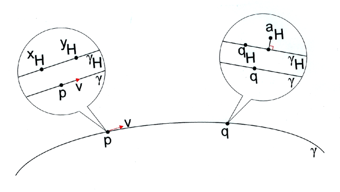
Figure 5.1. Microscopic images of a pair of infinitely close lines $\gamma$ and $\gamma_{H}$ on $M^{*}$

We continue with the proof by contradiction of Theorem 3.1. Let $H$ be an infinite Robinson hyperinteger (see Section 6, item 6.8). Then the sequence $({\mathcal{M}}_{n})$ is defined for the value $H$ of the index, by the extension principle (see Section 6, item 6.1). Note that by compactness of $M$, we have

$$M={\rm st}({\mathcal{M}}_{H}),$$ (5.1)

where “st” is the standard part function (see Section 6, item 6.3). Since the relation (3.2) is satisfied at all finite values of the index $n$, it is satisfied at the value $H$, as well, by the transfer principle (see Section 6, item 6.2). The points $x_{H}$ and $y_{H}$ are infinitely close to $p\in M$. The geodesic $\gamma_{H}$ passes through both $x_{H}$ and $y_{H}$ by construction, and is infinitely close to the limiting geodesic $\gamma$. By the transfer principle,

$$d(a_{H},q_{H})<\frac{1}{H}.$$

Equation (3.2) yields

$$|\iota_{H}(x)-\iota_{H}(y)|\leq(1-C)d(x_{H},y_{H}).$$ (5.2)

Let $\Delta s=d(x_{H},y_{H})$, so that $\gamma_{H}(\Delta s)=y_{H}$. Just as for a finite value of the index, we have

$$\alpha_{H}=\angle a_{H}x_{H}y_{H}.$$

The point $(x_{H},y_{H})$ is infinitely close to the point $(p,v)\in\hat{M}_{D}^{\times 2}$ of the blow-up constructed in Section 4. By Proposition 4.1, the function $F$ is continuous. Since $(x_{H},y_{H},a_{H})\approx((p,v),q)$, we have

$$F(x_{H},y_{H},a_{H})\approx F((p,v),q).$$ (5.3)

Therefore

$$\left|\frac{\Delta u_{H}}{\Delta s}\right|=F(x_{H},y_{H},a_{H})\approx F((p,v),q)=1,$$

and therefore

$$\frac{\Delta u_{H}}{\Delta s}\approx-1.$$ (5.4)

Note that by the transfer principle and the first variation (3.4), we obtain

$$u_{H}^{\prime}(0)=-\cos\alpha_{H},$$ (5.5)

but (5.4) is not immediate from (5.5), as the function $u_{H}$ is only internal rather than standard, so that one cannot apply (6.2) directly. Equation (5.4) is equivalent to

$$\frac{d(\gamma_{H}(\Delta s),a_{H})-d(x_{H},a_{H})}{\Delta s}\approx-1$$

or

$$\frac{d(y_{H},a_{H})-d(x_{H},a_{H})}{d(x_{H},y_{H})}\approx-1.$$

Thus an application of the standard part function “st” (see Section 6, item 6.3) yields

$${\rm st}\left(\frac{d(x_{H},a_{H})-d(y_{H},a_{H})}{d(x_{H},y_{H})}\right)=1,$$

contradicting (5.2). The resulting contradiction proves that some finite-dimensional imbedding will necesarily be $(1-C)$–bi-Lipschitz, completing the proof of Theorem 3.1.

6. A non-standard glossary

The present section is included mainly for the benefit of the reader not yet familiar with the general framework of non-standard analysis. The section can be omitted, shortened, or retained as is, as per recommendation of the referee.

A popular introduction to the subject may be found in [12], chapter 6: “Ghosts of departed quantities”.

In this section we present some illustrative terms and facts from non-standard calculus [8]. The relation of being infinitely close is denoted by the symbol $\approx$. Thus, $x\approx y$ if and only if $x-y$ is infinitesimal.

6.1. Natural hyperreal extension $f^{*}$

The construction of the hyperreals is carried out in the framework of the standard axiomatisation of set theory, denoted ZFC. Here ZFC stands for the axiom system of Zermelo and Fraenkel, with the addition of the Axiom of Choice.

The extension principle of non-standard calculus states that every real function $f$ has a hyperreal extension, denoted $f^{*}$ and called the natural extension of $f$. The transfer principle of non-standard calculus asserts that every real statement true for $f$, is true also for $f^{*}$. For example, if $f(x)>0$ for every real $x$ in its domain $I$, then $f^{*}(x)>0$ for every hyperreal $x$ in its domain $I^{*}$. Note that if the interval $I$ is unbounded, then $I^{*}$ necessarily contains infinite hyperreals. We will typically drop the star ^∗ so as not to overburden the notation.

6.2. Internal set

Internal set is the key tool in formulating the transfer principle, which concerns the logical relation between the properties of the real numbers ${\mathbb{R}}$, and the properties of a larger field denoted

$${\mathbb{R}}^{*}$$

called the hyperreal line. The field ${\mathbb{R}}^{*}$ includes, in particular, infinitesimal (“infinitely small”) numbers, providing a rigorous mathematical realisation of a project initiated by Leibniz. Roughly speaking, the idea is to express analysis over ${\mathbb{R}}$ in a suitable language of mathematical logic, and then point out that this language applies equally well to ${\mathbb{R}}^{*}$. This turns out to be possible because at the set-theoretic level, the propositions in such a language are interpreted to apply only to internal sets rather than to all sets. Note that the term “language” is used in a loose sense in the above. A more precise term is theory in first-order logic. Here a statement in first order logic by definition involves quantification only over elements (quantification over sets or sequences is not allowed).

Internal sets include natural extension of standard sets.

6.3. Standard part function

The standard part function “st” is the key ingredient in Abraham Robinson’s resolution of the paradox of Leibniz’s definition of the derivative as the ratio of two infinitesimals

$$\frac{dy}{dx}.$$

The standard part function associates to a finite hyperreal number $x$, the standard real $x_{0}$ infinitely close to it, so that we can write

$$\mathrm{st}(x)=x_{0}.$$

In other words, “st” strips away the infinitesimal part to produce the standard real in the cluster. The standard part function “st” is not defined by an internal set (see item 6.2 above) in Robinson’s theory.

6.4. Cluster

Each standard real is accompanied by a cluster of hyperreals infinitely close to it. The standard part function collapses the entire cluster back to the standard real contained in it. The cluster of the real number $0$ consists precisely of all the infinitesimals. Every infinite hyperreal decomposes as a triple sum

$$H+r+\epsilon,$$

where $H$ is a hyperinteger (see item 6.8 below), while $r$ is a real number in $[0,1)$, and $\epsilon$ is infinitesimal. Varying $\epsilon$ over all infinitesimals, one obtains the cluster of $H+r$.

6.5. Derivative

To define the derivative of $f$ in this approach, one no longer needs an infinite limiting process as in standard calculus. Instead, one sets

$$f^{\prime}(x)=\mathrm{st}\left(\frac{f(x+\epsilon)-f(x)}{\epsilon}\right),$$ (6.1)

where $\epsilon$ is infinitesimal, yielding the standard real number in the cluster of the hyperreal argument of “st”. Here the derivative exists if and only if the value (6.1) is independent of the choice of the infinitesimal. Note that

$$f^{\prime}(x)\approx\frac{f(x+\epsilon)-f(x)}{\epsilon}.$$ (6.2)

The addition of “st” to formula (6.1) resolves the centuries-old paradox famously criticized by George Berkeley [2] (in terms of the Ghosts of departed quantities, cf. [12, Chapter 6]), and provides a rigorous basis for the calculus.

6.6. Continuity

A function $f$ is continuous at $x$ if the following condition is satisfied: $y\approx x$ implies $f(y)\approx f(x)$.

6.7. Uniform continuity

A function $f$ is uniformly continuous on $I$ if the following condition is satisfied:

• standard: for every $\epsilon>0$ there exists a $\delta>0$ such that for all $x\in I$ and for all $y\in I$, if $|x-y|<\delta$ then $|f(x)-f(y)|<\epsilon$.

• non-standard: for all $x\in I^{*}$, if $x\approx y$ then $f(x)\approx f(y)$.

6.8. Hyperinteger

A hyperreal number $H$ equal to its own integer part

$$H=[H]$$

is called a hyperinteger (here the integer part function is the natural extension of the real one). The elements of the complement ${\mathbb{Z}}^{*}\setminus{\mathbb{Z}}$ are called infinite hyperintegers.

6.9. Proof of extreme value theorem

Let $H$ be an infinite hyperinteger. The interval $[0,1]$ has a natural hyperreal extension. Consider its partition into $H$ subintervals of equal length $\frac{1}{H}$, with partition points $x_{i}=i/H$ as $i$ runs from $0$ to $H$. Note that in the standard setting, with $n$ in place of $H$, a point with the maximal value of $f$ can always be chosen among the $n+1$ partition points $x_{i}$, by induction. Hence, by the transfer principle, there is a hyperinteger $i_{0}$ such that $0\leq i_{0}\leq H$ and

$$f(x_{i_{0}})\geq f(x_{i})\quad\forall i=0,...,H.$$ (6.3)

Consider the real point

$$c={\rm st}(x_{i_{0}}).$$

An arbitrary real point $x$ lies in a suitable sub-interval of the partition, namely $x\in[x_{i-1},x_{i}]$, so that ${\rm st}(x_{i})=x$. Applying “st” to the inequality (6.3), we obtain by continuity of $f$ that $f(c)\geq f(x)$, for all real $x$, proving $c$ to be a maximum of $f$ (see [8, p. 164] and [3, Chapter 12, p. 324]).

6.10. Limit

We have $\lim_{x\to a}f(x)=L$ if and only if whenever the difference $x-a$ is infinitesimal, the difference $f(x)-L$ is infinitesimal, as well, or in formulas: if ${\rm st}(x)=a$ then ${\rm st}(f(x))=L$.

Given a sequence of real numbers $\{x_{n}|n\in\mathbb{N}\}$, if $L\in\mathbb{R}\;$ we say $L$ is the limit of the sequence and write $L=\lim_{n\to\infty}x_{n}$ if the following condition is satisfied:

$${\rm st}(x_{H})=L\quad\mbox{\rm for all infinite }H$$ (6.4)

(here the extension principle is used to define $x_{n}$ for every infinite value of the index). This definition has no quantifier alternations. The standard $(\epsilon,\delta)$-definition of limit, on the other hand, does have quantifier alternations:

$$L=\lim_{n\to\infty}x_{n}\Longleftrightarrow\forall\epsilon>0\;,\exists N\in\mathbb{N}\;,\forall n\in\mathbb{N}:n>N\implies d(x_{n},L)<\epsilon.$$ (6.5)

References

- [1] Ambrosio, L.; Katz, M.: Flat currents modulo in metric spaces and filling radius inequalities, preprint.
- [2] Berkeley, George: The Analyst, a Discourse Addressed to an Infidel Mathematician (1734).
- [3] Ebbinghaus, H.-D.; Hermes, H.; Hirzebruch, F.; Koecher, M.; Mainzer, K.; Neukirch, J.; Prestel, A.; Remmert, R.: Numbers. With an introduction by K. Lamotke. Translated from the second 1988 German edition by H. L. S. Orde. Translation edited and with a preface by J. H. Ewing. Graduate Texts in Mathematics, 123. Readings in Mathematics. Springer-Verlag, New York, 1991.
- [4] Gromov, M.: Filling Riemannian manifolds. J. Diff. Geom., 18 (1983), 1–147.
- [5] Guth, L.: Notes on Gromov’s systolic estimate. Geom. Dedicata, 123 (2006), 113–129.
- [6] Kanovei, V.; Shelah, S.: A definable nonstandard model of the reals. J. Symbolic Logic 69 (2004), no. 1, 159–164.
- [7] Katz, M.: Systolic geometry and topology. With an appendix by Jake P. Solomon. Mathematical Surveys and Monographs, 137. American Mathematical Society, Providence, RI, 2007.
- [8] Keisler, H. Jerome: Elementary Calculus: An Infinitesimal Approach. Second Edition. Prindle, Weber & Schimidt, Boston, ’86.
- [9] Lightstone, A. H.: Infinitesimals. Amer. Math. Monthly 79 (1972), 242–251.
- [10] Robinson, Abraham: Non-standard analysis. North-Holland Publishing Co., Amsterdam 1966.
- [11] Robinson, Abraham: Non-standard analysis. Reprint of the second (1974) edition. With a foreword by Wilhelmus A. J. Luxemburg. Princeton Landmarks in Mathematics. Princeton University Press, Princeton, NJ, 1996.
- [12] Stewart, I.: From here to infinity. A retitled and revised edition of The problems of mathematics [Oxford Univ. Press, New York, 1992]. With a foreword by James Joseph Sylvester. The Clarendon Press, Oxford University Press, New York, 1996.