Dispersion interaction between crossed conducting wires

Abstract

We compute the $T=0K$ Van der Waals (nonretarded Casimir) interaction energy $E$ between two infinitely long, crossed conducting wires separated by a minimum distance $D$ much greater than their radius. We find that, up to a logarithmic correction factor, $E\propto-D^{-1}\left|\sin\theta\right|^{-1}f(\theta)$ where $f(\theta)$ is a smooth bounded function of the angle $\theta$ between the wires. We recover a conventional result of the form $E\propto-D^{-4}\left|\sin\theta\right|^{-1}g(\theta)$ when we include an electronic energy gap in our calculation.  Our prediction of gap-dependent energetics may be observable experimentally for carbon nanotubes, either via AFM detection of the vdW force or torque, or indirectly via observation of mechanical oscillations. This shows that strictly parallel wires, as assumed in previous predictions, are not needed to see a novel effect of this type.

At the micro- and nano-scale, dispersion (van der Waals, vdW) forces are ubiquitous Isra , and recent advances in manufacturing and measurement techniques have prompted much interest in their precise form.

The simplest theories sum vdW interaction energies between pairs of molecules, which is a good approximation for dilute insulating objects, where the dipole fluctuations at different points of one body are almost independent. For non-dilute dielectric and magnetic materials this summation approximation can be misleading, and may even give the wrong sign of the interaction Kenneth02 . Moreover, for anisotropic conducting nanostructures, the non-locality of Coulomb screening and associated density correlations within each object may change the form of the dispersive forces altogether Dobson06 ; CylsPlates .

This physics is exemplified by the class of quasi-1D objects, which exhibit correlation phenomena of both theoretical and experimental interest. Indeed, in the extreme limit truly confined $1D$ electrons experience a Luttinger liquid instability, as (e.g.) in single walled armchair nanotubes Egger .

When two such ”wires” are placed parallel and close to each other, the coulomb interaction between their density fluctuations may become a relevant perturbation, resulting in rich behavior at low temperatures and densities, such as locked charge density waves and Wigner cristallization. Klesse00 . The density density interaction is also responsible for coulomb drag phenomena whereby a current applied to one wire induces voltage on the other wire Hu ; Nazarov .

Dispersion forces between 1D systens are interesting even at larger separations. For the case of two infinitely long strictly parallel wires separated by distance $D$ greatly exceeding their radius $b$, the interaction energy is known Dobson06 ; Chang71 ; TanAnderson ; Matloob ; Drummond07 to be strongly dependent on the presence of an electronic energy gap:

$$E^{vdW}/L\propto-D^{-2}(\ln(D/b))^{-3/2}(metallic).$$ (1)

$$E^{vdW}/L\propto-D^{-5}(semiconducting)$$ (2)

The result (1) was obtained via zero-point energies of coupled plasmons in the random phase approximation (RPA), followed by a perturbative evaluation of the resulting integral Chang71 ; Dobson06 . The form (1) was also supported by diffusion Monte Carlo calculations Drummond07 .

Such forces may be important when one considers solutions of nanotubes or long molecules. Indeed, while ”wires” minimize their energy by aligning, in a solution of nanotubes a parallel configuration might not be formed because of entropic reasons. Therefore, it is important to understand the wire-wire interaction for a general orientation. Here we consider the angle and distance dependence for wires that are well separated. We will show that the (absolute) vdW energy of a pair of non-parallel wires inclined at angle $\theta$ is, up to a logarithmic correction factor specified later,

$$E^{vdW}\propto-D^{-1}\left|\sin\theta\right|^{-1}f(\theta)\;\;\;(metallic)$$ (3)

$$E^{vdW}\propto-D^{-4}\left|\sin\theta\right|^{-1}g(\theta)\;(semiconducting)$$ (4)

Here $D$ is the least distance between points on the two wires, and $\theta$ is the angle between the wires. $f$ and $g$ are smooth bounded functions. In this limit there is also a prospect of measuring the dispersion force between two nanotubes directly, via Atomic Force Microscopy (AFM) or spectroscopy of mechanical vibrations. Eqs (3,4) show that unusual gap-dependent results are expected from such experiments not only when the tubes are parallel Dobson06 , but also when they are non-parallel.

The crossed-wire interaction has previously been related to the interaction between anisotropic media in a similar manner to the way Casimir forces between molecules can be obtained from the Lifshitz formula by taking the dilute limit. The interaction between nonisotropic materials related to our problem was studied in Kenneth98 : there, the energy of a pair of media conducting only in prescribed (but different) directions is computed. In Rajter07 the interaction between non-isotropic dielectric media was considered and the limit of a dilute medium was associated with the interaction between a pairs of wires. The asymptotic results of Rajter07 were similar to those of a pair summation Parsegian approach (i.e. like Eq. (4)) even for metallic cases), and qualitatively different from Eq. (3)) derived below for metallic wires. We suspect that this difference may be due to the different Coulomb screening physics of a single pair of metallic wires compared to an infinite array of such wires. (See Gould09 for similar considerations relating to layered systems). This question is related to the very non-additive dispersion physics of low-dimensional, zero-gap systems in general Dobson06 .

In Emig08 , the orientational interaction between spheroidal dielectrics has been computed, but the metallic limit treated here was not yet considered. Some related work has also been done on 1D conductors in a collinear ”pointing” configuration White08 , but the calculation appropriate for metallic 1D conductors does not appear to have been done for cases where they are aligned in a non-parallel geometry.

Here we will compute the dispersion energy directly for crossed wires within second order perturbative non-retarded theory, as justified below. The interaction energy in this approach is (see e.g. Zaremba76 )

$$E^{(2)} =-\frac{\hbar}{2\pi}\int_{0}^{\infty}du\int d^{3}r_{1}d^{3}r_{2}d^{3}r_{1}^{\prime}d^{3}r_{2}^{\prime}V(r_{12})V(r_{1^{\prime}2^{\prime}})$$

$$\times\chi^{A}({\bf r}_{1},{\bf r}_{1}^{\prime},iu)\chi^{B}({\bf r}_{2},{\bf r}_{2}^{\prime},iu)$$

$$=-\hbar(2\pi)^{-7}\int d{\bf p}d{\bf p}^{\prime}\bar{V}(\left|{\bf p}\right|)V(\left|{\bf p}^{\prime}\right|)$$

$$\times\int_{0}^{\infty}du\chi^{(A)}(-{\bf p},-{\bf p}^{\prime},iu)\chi^{(B)}({\bf p},{\bf p}^{\prime},iu)$$ (6)

Here $\chi({\bf r},{\bf r}^{\prime})$ is the density-density response of each sub-system in the absence of the other sub-system, and $\chi({\bf p},{\bf p}^{\prime})$ is its 3D Fourier transform. $V({\bf r})$ is the bare Coulomb interaction between electrons in the two subsystems, and $V({\bf p})=4\pi e^{2}/|p|^{2}$ is its 3D Fourier transform. V can be considered small in the present case because of the large inter-wire separation assumed here. Indeed it is easily verified that (Dispersion interaction between crossed conducting wires) yields (1) for the case of parallel well-separated 1D conductors.

We consider a pair of wires $A,B$ described in Fig.1. One wire is assumed to lie along the $z$ axis. The xz plane and the origin are determined by demanding that the point on wire B, lying closest to wire A, is the point $(D,0,0).$ The orientation of wire B is then determined by a single angle $\theta.\;$

For later convenience we introduce unit vectors in the yz plane, parallel and perpendicular to wire $B$:  $\hat{u}=(0,\sin\theta,\cos\theta)$, $\hat{v}=(0,\cos\theta,-\sin\theta)$. Locations along wire A are denoted $z$, and locations along wire B are determined by a signed 1D position variable $s$ so that general points on wires A and B are  ${\bf R}_{A}(z)=(0,0,z)$,    ${\bf R}_{B}(s)=D\hat{x}+s\hat{u}$

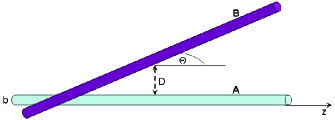
Figure 1: Van der Waals interaction of two crossed wires $A$ and $B$ at distance $D$ and angle $\theta$

The density-density response functions in 3D space of the two wires are written in terms of an assumed strictly 1D density-density response function $\bar{\chi}(z,\omega)$ for electron motion along a wire:

$$\chi^{(A)}({\bf r},{\bf r}^{\prime},\omega) =\bar{\chi}(z-z^{\prime},\omega)\delta(x)\delta(x^{\prime})\delta(y)\delta(y^{\prime})$$ (7)

$$\chi^{(B)}({\bf r},{\bf r}^{\prime},\omega) =\bar{\chi}(\left({\bf r}-{\bf r}^{\prime}\right)\cdot\hat{u},\omega)$$ (8)

$$\times\delta(x-D)\delta(x^{\prime}-D)\delta({\bf r}\cdot\hat{v})\delta({\bf r}^{\prime}\cdot\hat{v})$$

We express $\bar{\chi}(z,\omega)$ in terms of its 1D Fourier transform. $\bar{\chi}(z,\omega)=\frac{1}{2\pi}\int\bar{\chi}(q,\omega)\exp(iqz)dz$. Then, doubly Fourier-transforming (7) and (8) we obtain

$$\chi^{(A)}({\bf q},{\bf q}^{\prime}) =2\pi\int dk_{1}\bar{\chi}(k_{1},\omega)\delta(q_{z}+k_{1})\delta(q_{z}^{\prime}-k_{1})\;\;,$$ (9)

$$\chi^{(B)}({\bf q},{\bf q}^{\prime}) =2\pi\int dk_{2}\bar{\chi}(k_{2},\omega)\exp(i(q_{x}+q_{x}^{\prime})D)$$

$$\times\delta(\cos\theta q_{z}-\sin\theta q_{y}+k_{2})\delta(\cos\theta q_{z}^{\prime}-\sin\theta q_{y}^{\prime}-k_{2})$$

Putting (9,LABEL:ChiBqqp) into (6), and defining

$$F(k_{1},k_{2}) = \int_{0}^{\infty}\bar{\chi}(k_{1},iu)\bar{\chi}(k_{2},iu)du$$ (11)

$$V_{2D}(D,p) = 2\pi e^{2}\exp(-pD)/p$$ (12)

we obtain

$$E^{(2)} =-\frac{\hbar}{(2\pi)^{5}}\int dk_{2}dk_{1}d^{3}pd^{3}p^{\prime}F(k_{1},k_{2})V(\left|{\bf p}\right|)V(\left|{\bf p}^{\prime}\right|)$$

$$\times\exp(i(p_{x}+p_{x}^{\prime})D)\delta(k_{1}-p_{z})\delta(p_{z}^{\prime}+k_{1})$$

$$\times\delta(\cos\theta p_{z}-\sin\theta p_{y}+k_{2})\delta(\cos\theta p_{z}^{\prime}-\sin\theta p_{y}^{\prime}-k_{2})$$

$$=-\frac{\hbar}{\left(2\pi\right)^{3}} \int dk_{1}dk_{2}{F(k_{1},k_{2})\over\sin^{2}\theta}V_{2D}\Big{(}D,\sqrt{k_{1}^{2}+(-\frac{k_{1}\cos\theta+k_{2})}{\sin\theta})^{2}}\Big{)}^{2}.$$

We calculate the single-wire response $\bar{\chi}$ for eqs (11,LABEL:EZKAs2Dkintegral) within the Random Phase Approximation. From the work of Li and Das Sarma Li89 ,  this RPA approach for the long-wavelength collective motions can even be applied to a strongly interacting model of a 1D conducting system such as a Luttinger liquid. This would not apply for broken-symmetry cases such as a Wigner-crystalline wire, but this case is likely to occur only for small inter-wire separations Klesse00 , which are not the focus in the present work.

The starting point of the RPA for a single wire is the $bare$ density-density response $\bar{\chi}_{0}(k,\omega)$. The simplest model for $\bar{\chi}_{0}$ , at small $k$ and small $\omega=iu$, is

$$\bar{\chi}_{0}(k,iu)=-\frac{k^{2}n_{01D}}{m(u^{2}+\omega_{0}^{2})},$$ (14)

where $n_{01D}$ is the number of electrons per unit length in the ground state, and $m\,$is an appropriate mass. $\ \omega_{0}$ (with $\hbar\omega_{0}\approx$ Bloch energy gap $Eg$) is a harmonic pinning term allowing the modelling of both semiconducting and metallic wires.  We take $\omega_{0}=0$ for the metallic case, and $\omega_{0}\neq 0$ for semiconductors. (14) follows from classical motion of individual independent electrons ($F=ma$) but is also valid for the quantal motion of independent Fermions at small wavenumber $k$, corresponding, in the present case, to large interwire separation $D\sim k^{-1}$.

The Coulomb interaction $e^{2}/\left|z_{1}-z_{2}\right|$ between electrons on a strictly one-dimensional wire has a divergent Fourier transform corresponding to the region $z_{1}\rightarrow z_{2}$. In real quasi-1D structures such as carbon nanotubes there is a finite radius $b$ corresponding to the lateral spatial extent of the one-electron orbitals.  This serves to smear the Coulomb divergence at $z_{1}\rightarrow z_{2}$. The result depends on the detailed cross section assumed. For definiteness we choose a smeared Coulomb potential for electrons free to move on a cylindrical shell of zero thickness and radius $b$, representing a nanotube. The smeared intra-tube potential for this case is analytic:

$$v_{1D}(k) =2e^{2}I_{0}(|kb|)K_{0}(|kb|)$$ (15)

$$\approx 2e^{2}|ln(|kb|)|,\;\;for|kb|<<1.$$ (16)

where $I_{0}$, $K_{0}$ are modified Bessels. The long-wavelength form (16) is universal to all wire profiles but causes spurious collective modes and a divergent energy at larger k, requiring a cutoff to be imposed. Although the final result is highly insensitive to this cutoff, we preferred to use the specific form (15), thereby avoiding a cutoff altogether.

We now use the RPA  to write the long-wavelength response of mutually interacting quasi-1D electrons to an external potential as

$$\bar{\chi}(k,iu)=\frac{\bar{\chi}_{0}(k,iu)}{1-v_{1D}(k)\bar{\chi}_{0}(k,iu)}=\frac{n_{01D}k^{2}}{m(u^{2}+\Omega^{2}(k))}$$ (17)

$$\Omega^{2}(k)=\omega^{2}_{1D}(k)+\omega_{0}^{2}$$ (18)

Here $\omega_{1D}(k)$ is a quasi-acoustic 1D plasmon frequency, which can be written in terms of a 1D velocity $c_{1D}$ as

$$\omega_{1D}(k)=c_{1D}\left|k\right|\sqrt{I_{0}(|bk|)K_{0}(|bk|)},\;\;c_{1D}=\sqrt{2e^{2}n_{01D}/m}$$ (19)

Now the 1D plasmon group velocity $\partial\omega_{1D}/\partial q$ from (19) is much less than the speed of light $c$ except for $q<O(b^{-1}exp(-c^{2}/c_{1D}^{2}))$. Thus electromagnetic retardation can be ignored except at extremely large distances $D>>b\exp(c^{2}/c_{1D}^{2})$.

Puting (17) into (11)we find

$$F=\left(\frac{n_{01D}}{m}\right)^{2}\frac{\pi k_{1}^{2}k_{2}^{2}}{2\Omega(k_{1})\Omega(k_{2})\left\{\Omega(k_{1})+\Omega(k_{2})\right\}}$$ (20)

Case 1, conducting wires, $\omega_{0}=0$.

To analyze (LABEL:EZKAs2Dkintegral) we transform to dimensionless plane polar coordinates $(K,\phi)$:

$$k_{1}=D^{-1}Ksin(\phi+\frac{\theta}{2}),\;\;\;k_{2}=D^{-1}Ksin(\phi-\frac{\theta}{2})$$ (21)

with Jacobian $J=D^{-2}K/|sin(\theta)|$. This yields

$$E^{2:\;metal}=-\frac{\hbar c_{1D}}{16D|sin(\theta)|}h(\theta,r),\;\;\;r=b/D>>1$$ (22)

$$h(\theta,r)=\int_{0}^{\infty}dKe^{-2K}\int_{-\pi}^{\pi}d\phi\frac{s_{+}s_{-}}{\ell_{-}\ell_{+}\left(\ell_{-}s_{-}+\ell_{+}s_{+}\right)}$$ (23)

with $s_{\pm}\equiv\left|\sin(\phi\pm\frac{\theta}{2})\right|$ and $\ell_{\pm}=\sqrt{I_{0}(Krs_{\pm})K_{0}(Krs_{\pm})}$. Note that $h(\theta,r)$ is well behaved as $\theta\rightarrow 0$, with a limiting value $h(0,r)=(ln(D/b))^{-3/2}$ for $r\equiv b/D<<<1$.

For $r<<<1$ we thus obtain the analytic result

$$E^{(2)}\approx-\frac{1}{16D}\hbar c_{1D}\frac{1}{\left|\sin\theta\right|}\Big{(}\frac{1}{(\ln(D/b))^{3/2}}\Big{)}\;\;\;\;as\;\;\theta\rightarrow 0$$ (24)

For arbitrary $\theta$ and $r\equiv b/D<<1$ the function $h(\theta,r)$ defined by (23) requires numerical investigation. We define a smooth function $\Lambda$ with correct angular period:

$$\Lambda(\theta,r)\equiv h(\theta,r)(ln(1/r))^{3/2}\approx\sum_{n=0}^{N}c_{n}(r)cos(2n\theta)$$

$$c_{n}(r)\approx\frac{\sum_{i=0}^{\ell}a_{in}x^{i}}{1+\sum_{j=1}^{J}b_{jn}x^{j}},\;\;x=1/lnr$$ (25)

The choices $N=5,I=3,J=2$ give a good fit to (23) for $x<0.4$, i.e. for $D/b\equiv r^{-1}>16.5$, and the corresponding coefficients $a,b$ are given in Table 1.

$a_{in}$	n=0	n=1	n=2	n=3	n=4	n=5
i=0	0.85708	0.11770	0.01534	0.00453	0.00189	0.00097
i=1	0.18049	0.19040	0.04743	0.01538	0.04505	0.00228
i=2	2.85682	0.51752	0.12230	0.03615	0.01378	0.00783
i=3	2.78324	0.61964	0.13410	0.03497	0.03237	0.01795
$b_{jn}$	n=0	n=1	n=2	n=3	n=4	n=5
j=1	-2.29966	-0.24097	-0.06158	-0.00820	-0.00657	-0.00357
j=2	2.47243	-0.19977	0.70113	0.91201	0.95313	0.97461

Table 1: Coefficients for log-cosine expansion (25) of $\Lambda(\theta,r)$

Case 2, semiconducting wires, $\omega_{0}\neq 0$. Here there are two analytic cases according to the separation D: either of the terms on the right of (18) could dominate for the $k$ values $k\approx D^{-1}$ that dominate the energy integral (LABEL:EZKAs2Dkintegral).

Case 2a, smaller separations When

$$D<<D_{0}\equiv c_{1D}\omega_{0}^{-1}\sqrt{ln(c_{1D}/(\omega_{0}b))}$$ (26)

we can again ignore $\omega_{0}$ in (18), thus recovering the ”metallic” vdW energy (22). Because of our large-separation approximations, this conclusion only holds provided that $D_{0}$ from (26) satisfies $D_{0}>>b$, which can occur for very small gaps $\omega_{0}$ such as that noted for (9,3) nanotubes in Rajter07 .

Case 2b, larger separations $D>>D_{0}$ Here we can ignore the $\omega_{P1D}^{2}$ term in (18) for the relevant values $k\approx 1/D$. Then (11) becomes $F\approx\left(\frac{n_{01D}}{m}\right)^{2}k_{1}^{2}k_{2}^{2}\frac{\pi/2}{2\omega_{0}^{3}}$ and using (21), we evaluate (LABEL:EZKAs2Dkintegral) as

$$E^{(2):semicond} = -\frac{3\pi}{1024}\frac{1}{D^{4}}\frac{\hbar c_{1D}^{4}}{\omega_{0}^{3}}\frac{2\cos^{2}\theta+1}{\left|\sin\theta\right|}$$ (27)

This is consistent with Eq (57) of Rajter07 .

Conclusions: Eq (22) is the principal result of the present work, along with (23) and (25). It shows that nonparallel conducting wires experience a vdW attractive energy that decays much more slowly with distance $D$ than the standard $D^{-4}$ dependence predicted by summing $R_{ij}^{-6}$ contributions over all elements $i,j$ of the wires. (22) also shows a strong angular dependence, giving rise to significant slowly-decaying vdW torques.

The interaction predicted here might be measured directly in Atomic Force Microscopy experiments on metallic carbon nanotubes, or indirectly via their mechanical vibrations. In Figure 2 we estimate the force $F^{met}$ between the conduction-band electrons of two freestanding metallic (5,5) carbon nanotubes in vacuo, as a function of separation $D$, both for strictly parallel tubes of length 1 micron using Eq. (1) of Dobson06 , and for infinitely long tubes at angle $\theta=1^{0}$ from Eq. (22). $F^{ins}\propto D^{-6}$ is the dispersion force from the remaining insulating electron bands via the usual pairwise summation approach using data from Saito and UnivGraphPot . For comparison, $F^{e-e}$ gives the force between two localized (impurity) single-electron charges separated by $D$. The dispersion force $F^{disp}=F^{met}+F^{ins}$ could be distinguished from that due to any localised extra electrons because $F^{disp}$, unlike $F^{e-e}$, will be invariant when one tube is made to slide along its own length.

	$F^{met}\hfill\vline$	$F^{ins}\hfill\vline$	$F^{met}\hfill\vline$	$F^{ins}$	$F^{e-e}$
	L=1 $\mu$	L=1 $\mu$	$L\rightarrow\infty$	$L\rightarrow\infty$
D(nm)	$\theta=0$	$\theta=0$	$\theta=1^{0}$	$\theta=1^{0}$
2	250	1370	41	205	57.6
5	9.3	5.6	3.6	2.1	9.2
10	0.85	0.088	0.7	0.065	2.3

Figure 2: vdW Force contributions in picoNewtons between (5,5) CNTs (1st 4 columns) and Coulomb force between two electrons.

We note finally that the present theoretical results can be understood in terms of long-wavelength collective excitations, and are not limited to $T=0K$. However in practice $T$ needs to be low enough for a long electronic mean free path $>D$ to be maintained.

J. D. and I. K. acknowledge the hospitality of KITP and partial support from the NSF under Grant No. PHY05-51164. J. D. and T. G. were supported by the CSIRO National Hydrogen Materials Alliance. Discussions with R. Podgornik, A. Parsegian, M. Kardar, T. Emig and R. French were much appreciated.

References

- (1) J. N. Israelachvili, Intermolecular and Surface Forces (Academic Press, London, 1992).
- (2) O. Kenneth, I. Klich, A. Mann, and M. Revzen, Phys. Rev. Lett. 89, 033001 (2002).
- (3) J. F. Dobson, A. White, and A. Rubio, Phys. Rev. Lett. 96, 073201 (2006).
- (4) S. J. Rahi, T. Emig, R. L. Jaffe, and M. Kardar, Phys. Rev. A 78, 012014 (2008).
- (5) R. Egger and A. Gogolin, Phys. Rev. Lett. 79, 5082 (1997).
- (6) R. Klesse and A. Stern, Phys. Rev. B 62, 16912 (2000).
- (7) B. Y.-K. Hu and K. Flensberg, in Hot Carriers in Semiconductors, edited by K. Hess (Plenum, New York, 1996).
- (8) Y. V. Nazarov and D. V. Averin, Phys. Rev. Lett. 81, 653 (1998).
- (9) D. B. Chang, R. L. Cooper, J. E. Drummond, and A. C. Young, Phys. Letts. 37A, 311 (1971).
- (10) S. L. Tan and P. W. Anderson, Chem. Phys. Lett. 97, 23 (1983).
- (11) R. Matloob, A. Keshavarz, and D. Sedighi, Phys. Rev. A 60, 3410 (1999).
- (12) N. D. Drummond and R. J. Needs, Phys. Rev. Lett. 99, 166401 (2007).
- (13) O. Kenneth, hep-th/9802149 (1998).
- (14) R. F. Rajter, R. Podgornik, V. A. Parsegian, R. H. French, and W. Y. Ching, Phys. Rev. B 76, 045417 (2007).
- (15) V. A. Parsegian, Van der Waals Forces (Cambridge University Press, Cambridge, 2006).
- (16) T. Gould, E. M. Gray, and J. F. Dobson, Phys. Rev. B 79, 113402 (2009).
- (17) T. Emig, N. Graham, R. L. Jaffe, and M. Kardar, arXiv:0811.1597 (2008).
- (18) A. White and J. F. Dobson, Phys. Rev. B 77, 075436 (2008).
- (19) E. Zaremba and W. Kohn, Phys. Rev. B 13, 2270 (1976).
- (20) Q. Li and S. Das Sarma, Phys. Rev. B 40, 5860 (1989).
- (21) R. Saito, G. Dresselhaus, and M. Dresselhaus, Physical Properties of Carbon Nanotubes (Imperial College Press, London, 1998).
- (22) L. A. Girifalco, M. Hodak, and R. S. Lee, Phys. Rev. B 62, 13104 (2000).