Parton distributions in the virtual photon target
up to NNLO in QCD

Abstract

Parton distributions in the virtual photon target are investigated in perturbative QCD up to the next-to-next-to-leading order (NNLO). In the case $\Lambda^{2}\ll P^{2}\ll Q^{2}$, where $-Q^{2}$ ($-P^{2}$) is the mass squared of the probe (target) photon, parton distributions can be predicted completely up to the NNLO, but they are factorisation-scheme-dependent. We analyse parton distributions in two different factorisation schemes, namely $\overline{\rm MS}$ and ${\rm DIS}_{\gamma}$ schemes, and discuss their scheme dependence. We show that the factorisation-scheme dependence is characterised by the large-$x$ behaviours of quark distributions. Gluon distribution is predicted to be very small in absolute value except in the small-$x$ region.

I Introduction

It is well known that, in $e^{+}e^{-}$ collision experiments, the cross section for the two-photon processes $e^{+}e^{-}\rightarrow e^{+}e^{-}+{\rm hadrons}$ illustrated in Fig.1 dominates at high energies over other processes such as the one-photon annihilation process $e^{+}e^{-}\rightarrow\gamma^{*}\rightarrow{\rm hadrons}$. The two-photon processes are observed in the double-tag events where both the outgoing $e^{+}$ and $e^{-}$ are detected. Especially, the case in which one of the virtual photon is far off-shell (large $Q^{2}\equiv-q^{2}$), while the other is close to the mass-shell (small $P^{2}=-p^{2}$), can be viewed as a deep-inelastic scattering where the target is a photon rather than a nucleon WalshBKT . In this deep-inelastic scattering off photon targets, we can study the photon structure functions, which are the analogues of the nucleon structure functions.

Figure 1: Deep inelastic scattering on a virtual photon in the $e^{+}~{}e^{-}$ collider experiments.

A unique and interesting feature of the photon structure functions is that, in contrast with the nucleon case, the target mass squared $P^{2}$ is not fixed but can take various values and that the structure functions show different behaviours depending on the values of $P^{2}$.

In the case of a real photon target ($P^{2}=0$), unpolarised (spin-averaged) photon structure functions $F_{2}^{\gamma}(x,Q^{2})$ and $F_{L}^{\gamma}(x,Q^{2})$ were studied first in the parton model WalshZerwas , and then investigated in perturbative QCD (pQCD). In the framework based on the operator product expansion (OPE) CHM supplemented by the renormalisation (RG) group method, Witten Witten obtained the leading order (LO) QCD contributions to $F_{2}^{\gamma}$ and $F_{L}^{\gamma}$ and, shortly after, the next-to-leading order (NLO) QCD contributions were calculated by Bardeen and Buras BB . The same results were rederived by the QCD improved parton model powered by the parton evolution equations Dewitt ; GR . Recently, some of the parameters which are necessary to evaluate the next-to-next-to-leading order (NNLO) corrections to $F_{2}^{\gamma}$ were calculated and also the NNLO solution of the evolution equations for the real photon case was dealt with MVV . When polarised beams are used in $e^{+}e^{-}$ collision experiments, we can get information on the spin structure of the photon. The QCD analysis of the polarised photon structure function $g_{1}^{\gamma}(x,Q^{2})$ for the real photon target was performed in the LO KS and in the NLO SV ; GRS . For more information on the recent theoretical and experimental investigation of unpolarised and polarised photon structure, see the review articles Krawczyk .

For a virtual photon target ($P^{2}\neq 0$), we obtain the virtual photon structure functions $F_{2}^{\gamma}(x,Q^{2},P^{2})$ and $F_{L}^{\gamma}(x,Q^{2},P^{2})$. They were studied in the LO UW1 and in the NLO UW2 by pQCD. In fact, these structure functions were analysed in the kinematical region,

$$\Lambda^{2}\ll P^{2}\ll Q^{2}~{},$$ (1)

where $\Lambda$ is the QCD scale parameter. The advantage of studying a virtual photon target in this kinematical region (1) is that we can calculate the whole structure function, its shape and magnitude, by the perturbative method. This is contrasted with the case of the real photon target where in the NLO and beyond there appear nonperturbative pieces. The virtual photon structure functions $F_{2}^{\gamma}$ and $F_{L}^{\gamma}$ were also studied by the QCD improved parton model Rossi ; DG ; GRStratmann ; Fontannaz . In the same kinematical region (1), the polarised virtual photon structure function $g_{1}^{\gamma}(x,Q^{2},P^{2})$ was investigated up to the NLO in pQCD SU1 , and its target mass effects were studied BSU . Moreover, the first moment of $g_{1}^{\gamma}(x,Q^{2},P^{2})$ was calculated up to the NNLO SUU .

Recently the three-loop calculations were made for the anomalous dimensions of both quark and gluon operators MVV1 ; MVV2 and also for the photon-quark and photon-gluon splitting functions MVV3 . Using these results, we analysed the virtual photon structure functions $F_{2}^{\gamma}(x,Q^{2},P^{2})$ and $F_{L}^{\gamma}(x,Q^{2},P^{2})$ in the kinematical region (1) in QCD. We could give definite predictions for $F_{2}^{\gamma}(x,Q^{2},P^{2})$ up to the NNLO and for $F_{L}^{\gamma}(x,Q^{2},P^{2})$ up to the NLO USU , and also for the target mass effects on these functions KSUU .

In parton picture, structure functions are expressed as convolutions of coefficient functions and parton distributions in the target. And these parton distributions will be used for predicting the behaviours of other processes. When the target is a virtual photon with $P^{2}$ being in the kinematical region (1), then a definite prediction can be made for its parton distributions in pQCD. However, it is well known that parton distributions are dependent on the scheme which is employed to factorise structure functions into coefficient functions and parton distributions. It is possible that parton distributions obtained in one factorisation scheme may be more appropriate to use than those acquired in other schemes. Indeed, for the case of the polarised virtual photon target, the NLO QCD analysis was made for its parton distributions in several factorisation schemes and their scheme dependence was closely studied SU2 .

In this paper we perform the QCD analysis of the parton distributions in the unpolarised virtual photon target up to the NNLO. We investigate the distributions of the flavour singlet and nonsinglet quarks and gluons in two factorisation schemes, namely $\overline{\rm MS}$ and ${\rm DIS}_{\gamma}$ schemes. Using the framework of the QCD improved parton model, we give, in the next section, the explicit expressions for the moments of the flavour singlet (nonsinglet) quark and gluon distributions up to the NNLO. In Sec.III, we show first that the parton distributions obtained up to the NNLO are independent of the renormalisation-prescription which is chosen in defining the QCD coupling constant $\alpha_{s}$. And then we explain the two factorisation schemes, $\overline{\rm MS}$ and ${\rm DIS}_{\gamma}$ schemes, which we consider in this paper. The behaviours of the parton distributions near $x=1$ and their factorisation-scheme dependence are discussed in Sec.IV. The numerical analysis of the parton distributions predicted by $\overline{\rm MS}$ and ${\rm DIS}_{\gamma}$ schemes will be given in Sec.V. The final section is devoted to the conclusion.

II Parton distributions in the virtual photon

In this section the parton distributions in the virtual photon are analysed in the framework of the QCD improved parton model Altarelli with the DGLAP parton evolution equations.

Let $q^{i}_{\pm}(x,Q^{2},P^{2})$, $G^{\gamma}_{\pm}(x,Q^{2},P^{2})$, $\Gamma^{\gamma}_{\pm}(x,Q^{2},P^{2})$ be quark with $i$-flavour, gluon, and photon distribution functions with $\pm$ helicities in the virtual photon with mass $-P^{2}$. Then the spin-averaged parton distributions in the virtual photon are defined as

$$q^{i} \equiv \frac{1}{2}[q^{i}_{+}+{\overline{q}}^{i}_{+}+q^{i}_{-}+{\overline{q}}^{i}_{-}]~{},$$

$$G^{\gamma} \equiv \frac{1}{2}[G^{\gamma}_{+}+G^{\gamma}_{-}]~{},\qquad\Gamma^{\gamma}\equiv\frac{1}{2}[\Gamma^{\gamma}_{+}+\Gamma^{\gamma}_{-}]~{}.$$ (2)

In the leading order of the electromagnetic coupling constant, $\alpha=e^{2}/4\pi$, $\Gamma^{\gamma}$ does not evolve with $Q^{2}$ and is set to be

$$\Gamma^{\gamma}(x,Q^{2},P^{2})=\delta(1-x)~{}.$$ (3)

Instead of using the quark distributions $q^{i}$, it is advantageous to treat the flavour singlet and nonsinglet combinations defined as follows:

$$q^{\gamma}_{S} \equiv \sum_{i}~{}q^{i}~{},$$ (4)

$$q^{\gamma}_{NS} \equiv \sum_{i}e^{2}_{i}\Bigl{(}q^{i}-\frac{q^{\gamma}_{S}}{n_{f}}\Bigr{)}~{},$$ (5)

where $n_{f}$ is the number of relevant active quark (i.e., the massless quark) flavours and $e_{i}$ is the electromagnetic charge of the active quark with flavour $i$ in the unit of proton charge.

Now introducing a row vector

$$\bm{q}^{\gamma}=(q^{\gamma}_{S},~{}G^{\gamma},~{}q^{\gamma}_{NS}),$$ (6)

the parton distributions $\bm{q}^{\gamma}(x,Q^{2},P^{2})$ in the virtual photon satisfy an inhomogeneous evolution equation Dewitt ; GR ; MVV

$$\frac{d~{}\bm{q}^{\gamma}(x,Q^{2},P^{2})}{d~{}\ln Q^{2}}=\bm{k}(x,Q^{2})+\int_{x}^{1}\frac{dy}{y}\bm{q}^{\gamma}(y,Q^{2},P^{2})P(\frac{x}{y},Q^{2})~{},$$ (7)

where the elements of a row vector $\bm{k}=(k_{S},~{}k_{G},~{}k_{NS})$ refer to the splitting functions of $\gamma$ to the singlet quark combination, to gluon and to nonsinglet quark combination, respectively. The $3\times 3$ matrix $P(z,Q^{2})$ is expressed as

$$P(z,Q^{2})=\begin{pmatrix}P^{S}_{qq}(z,Q^{2})&P_{Gq}(z,Q^{2})&0\\ P_{qG}(z,Q^{2})&P_{GG}(z,Q^{2})&0\\ 0&0&P^{NS}_{qq}(z,Q^{2})\end{pmatrix}~{},$$ (8)

where $P_{AB}$ is a splitting function of $B$-parton to $A$-parton.

There are two methods to obtain the parton distribution $\bm{q}^{\gamma}(x,Q^{2},P^{2})$ up to the NNLO. In one method, we use the parton splitting functions up to the three-loop level and we solve numerically $\bm{q}^{\gamma}(x,Q^{2},P^{2})$ in Eq.(7) by iteration, starting from the initial quark and gluon distributions of the virtual photon at $Q^{2}=P^{2}$. The interesting point of studying the virtual photon with mass $-P^{2}$ is that when $P^{2}\gg\Lambda^{2}$, the initial parton distributions of the photon are completely known up to the two-loop level in QCD. The other method, which is more common than the former, is by making use of the inverse Mellin transformation. From now on we follow the latter method. First we take the Mellin moments of Eq.(7),

$$\frac{d~{}\bm{q}^{\gamma}(n,Q^{2},P^{2})}{d~{}\ln Q^{2}}=\bm{k}(n,Q^{2})+\bm{q}^{\gamma}(n,Q^{2},P^{2})P(n,Q^{2})~{},$$ (9)

where we have defined the moments of an arbitrary function $f(x)$ as

$$f(n)\equiv\int_{0}^{1}dxx^{n-1}f(x).$$ (10)

Henceforce we omit the obvious $n$-dependence for simplicity. Expansions are made for the splitting functions $\bm{k}(Q^{2})$ and $P(Q^{2})$ in powers of the QCD and QED coupling constants as follows:

$$\bm{k}(Q^{2}) = \frac{\alpha}{2\pi}\bm{k}^{(0)}+\frac{\alpha\alpha_{s}(Q^{2})}{(2\pi)^{2}}\bm{k}^{(1)}+\frac{\alpha}{2\pi}\left[\frac{\alpha_{s}(Q^{2})}{2\pi}\right]^{2}\bm{k}^{(2)}\cdots~{},$$ (11)

$$P(Q^{2}) = \frac{\alpha_{s}(Q^{2})}{2\pi}P^{(0)}+\left[\frac{\alpha_{s}(Q^{2})}{2\pi}\right]^{2}P^{(1)}+\left[\frac{\alpha_{s}(Q^{2})}{2\pi}\right]^{3}P^{(2)}+\cdots~{},$$ (12)

and a new variable $t$ is introduced as the evolution variable instead of $Q^{2}$ FP1 ,

$$t\equiv\frac{2}{\beta_{0}}\ln\frac{\alpha_{s}(P^{2})}{\alpha_{s}(Q^{2})}~{}.$$ (13)

The solution $\bm{q}^{\gamma}(t)(=\bm{q}^{\gamma}(n,Q^{2},P^{2}))$ of Eq.(9) is decomposed in the following form:

$$\bm{q}^{\gamma}(t)=\bm{q}^{\gamma(0)}(t)+\bm{q}^{\gamma(1)}(t)+\bm{q}^{\gamma(2)}(t)~{},$$ (14)

where the first, second and third terms represent the solution in the LO, NLO and NNLO, respectively. Then they satisfy the following three differential equations:

$$\frac{d{\bm{q}}^{\gamma(0)}(t)}{dt} = \frac{\alpha}{\alpha_{s}(t)}{\bm{k}}^{(0)}+{\bm{q}}^{\gamma(0)}(t)P^{(0)}~{},$$ (15)

$$\frac{d{\bm{q}}^{\gamma(1)}(t)}{dt} = \frac{\alpha}{2\pi}~{}\bm{R}_{K(1)}+\frac{\alpha_{s}(t)}{2\pi}~{}{\bm{q}}^{\gamma(0)}(t)~{}R_{P(1)}+{\bm{q}}^{\gamma(1)}(t)P^{(0)}~{},$$ (16)

$$\frac{d{\bm{q}}^{\gamma(2)}(t)}{dt} = \frac{\alpha}{2\pi}\frac{\alpha_{s}(t)}{2\pi}~{}\bm{R}_{K(2)}+\Bigl{(}\frac{\alpha_{s}(t)}{2\pi}\Bigr{)}^{2}~{}{\bm{q}}^{\gamma(0)}(t)~{}R_{P(2)}$$ (17)

$$\qquad+\frac{\alpha_{s}(t)}{2\pi}~{}{\bm{q}}^{\gamma(1)}(t)~{}R_{P(1)}+{\bm{q}}^{\gamma(2)}(t)P^{(0)}~{},$$

where

$$\bm{R}_{K(1)} = \bm{k}^{(1)}-\frac{\beta_{1}}{2\beta_{0}}\bm{k}^{(0)}~{},$$ (18)

$$R_{P(1)} = P^{(1)}-\frac{\beta_{1}}{2\beta_{0}}P^{(0)}~{},$$ (19)

$$\bm{R}_{K(2)} = {\bm{k}}^{(2)}-\frac{\beta_{1}}{2\beta_{0}}{\bm{k}}^{(1)}+\frac{1}{4}\Bigl{(}(\frac{\beta_{1}}{\beta_{0}})^{2}-\frac{\beta_{2}}{\beta_{0}}\Bigr{)}{\bm{k}}^{(0)}~{},$$ (20)

$$R_{P(2)} = P^{(2)}-\frac{\beta_{1}}{2\beta_{0}}P^{(1)}+\frac{1}{4}\Bigl{(}(\frac{\beta_{1}}{\beta_{0}})^{2}-\frac{\beta_{2}}{\beta_{0}}\Bigr{)}P^{(0)}~{}.$$ (21)

where we have used the fact the QCD effective coupling constant $\alpha_{s}(Q^{2})$ satisfies

$$\frac{d\alpha_{s}(Q^{2})}{d{\rm ln}Q^{2}}=-\beta_{0}\frac{\alpha_{s}(Q^{2})^{2}}{4\pi}-\beta_{1}\frac{\alpha_{s}(Q^{2})^{3}}{(4\pi)^{2}}-\beta_{2}\frac{\alpha_{s}(Q^{2})^{4}}{(4\pi)^{3}}+\cdots,$$ (22)

where $\beta_{0}=11-\frac{2}{3}n_{f}$  and $\beta_{1}$ and $\beta_{2}$ were known  JC ; TVZ . Note that the $P^{2}$ dependence of $\bm{q}^{\gamma}$ solely comes from the initial condition (or boundary condition) as we will see below.

The initial conditions for $\bm{q}^{\gamma(0)}$, $\bm{q}^{\gamma(1)}$ and $\bm{q}^{\gamma(2)}$ are obtained as follows: For $-p^{2}=P^{2}\gg\Lambda^{2}$, the photon matrix elements of the hadronic operators $O_{n}^{i}$ ($i=S~{}({\rm or}\ \psi),G,NS$) can be calculated perturbatively. Renormalising at $\mu^{2}=P^{2}$, we obtain at two-loop level

$$\langle\gamma(p)\mid O_{n}^{i}(\mu)\mid\gamma(p)\rangle|_{\mu^{2}=P^{2}}=\frac{\alpha}{4\pi}\Bigl{\{}{\widetilde{A}}_{n}^{i(1)}+\frac{\alpha_{s}(P^{2})}{4\pi}{\widetilde{A}}_{n}^{i(2)}\Bigr{\}},\quad i=S~{}({\rm or}\ \psi),G,NS~{}.$$ (23)

The ${\widetilde{A}}_{n}^{i(1)}$ and ${\widetilde{A}}_{n}^{i(2)}$ terms represent the operator mixing between the hadronic operators and photon operators in the NLO and NNLO, respectively, and the operator mixing implies that there exist parton distributions in the photon. Thus we have, at $\mu^{2}=P^{2}$ (or at $t=0$),

$$\bm{q}^{\gamma(0)}(0)=\bm{0},\qquad\bm{q}^{\gamma(1)}(0)=\frac{\alpha}{4\pi}{\widetilde{\bm{A}}}_{n}^{(1)},\qquad\bm{q}^{\gamma(2)}(0)=\frac{\alpha\alpha_{s}(P^{2})}{(4\pi)^{2}}{\widetilde{\bm{A}}}_{n}^{(2)},$$ (24)

with

$${\widetilde{\bm{A}}}_{n}^{(l)}=\Bigl{(}{\widetilde{A}}_{n}^{S(l)},{\widetilde{A}}_{n}^{G(l)},{\widetilde{A}}_{n}^{NS(l)}\Bigr{)}~{},\qquad l=1,2~{}.$$ (25)

Actually, the initial quark distributions emerge in the NLO (the order $\alpha$) and gluon distribution in the NNLO (the order $\alpha\alpha_{s}$). The expressions of ${\widetilde{\bm{A}}}_{n}^{(1)}$ and ${\widetilde{\bm{A}}}_{n}^{(2)}$ in $\overline{\rm MS}$ scheme are enumerated in Appendix A.1.

With these initial conditions, the solutions ${\bm{q}}^{\gamma(0)}(t)$, ${\bm{q}}^{\gamma(1)}(t)$ and ${\bm{q}}^{\gamma(2)}(t)$ are given by

$${\bm{q}}^{\gamma(0)}(t) = \frac{4\pi}{\alpha_{s}(t)}~{}\bm{a}~{}\biggl{\{}{\bm{1}}-\biggl{[}\frac{\alpha_{s}(t)}{\alpha_{s}(0)}\biggr{]}^{1-\frac{2P^{(0)}}{\beta_{0}}}\biggr{\}}~{},$$ (26)

$${\bm{q}}^{\gamma(1)}(t) = \biggl{[}\frac{\alpha}{2\pi}~{}{\bm{R}}_{K(1)}+2\bm{a}~{}R_{P(1)}\biggr{]}\frac{-1}{P^{(0)}}~{}\biggl{\{}{\bm{1}}-\biggl{[}\frac{\alpha_{s}(t)}{\alpha_{s}(0)}\biggr{]}^{-\frac{2P^{(0)}}{\beta_{0}}}\biggr{\}}$$

$$-2~{}\bm{a}~{}\biggl{\{}\int^{t}_{0}d\tau e^{(P^{(0)}-\frac{\beta_{0}}{2})\tau}~{}R_{P(1)}~{}e^{-P^{(0)}\tau}\biggr{\}}~{}e^{P^{(0)}t}+{\bm{q}}^{\gamma(1)}(0)\biggl{[}\frac{\alpha_{s}(t)}{\alpha_{s}(0)}\biggr{]}^{-\frac{2P^{(0)}}{\beta_{0}}}~{},$$

$${\bm{q}}^{\gamma(2)}(t) = \frac{\alpha_{s}(t)}{2\pi}\Biggl{\{}\Bigl{[}\frac{\alpha}{2\pi}~{}{\bm{R}}_{K(2)}+2{\bm{a}}~{}R_{P(2)}\Bigr{]}\frac{-1}{\frac{\beta_{0}}{2}+P^{(0)}}\biggl{\{}{\bm{1}}-\biggl{[}\frac{\alpha_{s}(t)}{\alpha_{s}(0)}\biggr{]}^{-1-\frac{2P^{(0)}}{\beta_{0}}}\biggr{\}}$$ (28)

$$\hskip 34.14322pt-2{\bm{a}}\biggl{\{}\int^{t}_{0}d\tau e^{(P^{(0)}-\frac{\beta_{0}}{2})\tau}~{}R_{P(2)}~{}e^{-(\frac{\beta_{0}}{2}+P^{(0)})\tau}\biggr{\}}e^{(\frac{\beta_{0}}{2}+P^{(0)})t}$$

$$\hskip 34.14322pt+\Bigl{[}\frac{\alpha}{2\pi}~{}{{\bm{R}}}_{K(1)}+2{\bm{a}}~{}R_{P(1)}\Bigr{]}\frac{-1}{P^{(0)}}$$

$$\hskip 113.81102pt\times\biggl{\{}\int^{t}_{0}d\tau\Bigl{[}{\bm{1}}-e^{P^{(0)}\tau}\Bigr{]}R_{P(1)}~{}e^{-(\frac{\beta_{0}}{2}+P^{(0)})\tau}\biggr{\}}e^{(\frac{\beta_{0}}{2}+P^{(0)})t}$$

$$\hskip 34.14322pt-2~{}{\bm{a}}\biggl{\{}\int^{t}_{0}d\tau\biggl{[}\int^{\tau}_{0}d\tau^{\prime}e^{(P^{(0)}-\frac{\beta_{0}}{2})\tau^{\prime}}~{}R_{P(1)}~{}e^{-P^{(0)}\tau^{\prime}}\biggr{]}$$

$$\hskip 113.81102pt\times e^{P^{(0)}\tau}R_{P(1)}~{}e^{-(\frac{\beta_{0}}{2}+P^{(0)})\tau}\biggr{\}}e^{(\frac{\beta_{0}}{2}+P^{(0)})t}$$

$$\hskip 34.14322pt+{\bm{q}}^{\gamma(1)}(0)\biggl{\{}\int^{t}_{0}d\tau e^{P^{(0)}\tau}R_{P(1)}~{}e^{-(\frac{\beta_{0}}{2}+P^{(0)})\tau}\biggr{\}}e^{(\frac{\beta_{0}}{2}+P^{(0)})t}\Biggr{\}}$$

$$\hskip 34.14322pt+{\bm{q}}^{\gamma(2)}(0)~{}\biggl{[}\frac{\alpha_{s}(t)}{\alpha_{s}(0)}\biggr{]}^{-\frac{2P^{(0)}}{\beta_{0}}},$$

where

$$\bm{a}=\frac{\alpha}{2\pi\beta_{0}}\bm{k}^{(0)}\frac{1}{1-\frac{2P^{(0)}}{\beta_{0}}}~{}.$$ (29)

For the case of the real photon target, the NLO solution ${\bm{q}}^{\gamma(1)}(t)$ was given in GR (see also FP2 ) and the NNLO solution ${\bm{q}}^{\gamma(2)}(t)$ in MVV .

The moments of the splitting functions are related to the anomalous dimensions of operators as follows USU :

$$P^{(0)} = -\frac{1}{4}\widehat{\gamma}^{(0)}_{n}~{},\qquad P^{(1)}=-\frac{1}{8}\widehat{\gamma}^{(1)}_{n}~{},\qquad P^{(2)}=-\frac{1}{16}\widehat{\gamma}^{(2)}_{n}~{},$$

$${\bm{k}}^{(0)} = \frac{1}{4}{\bm{K}}^{(0)}_{n},\qquad{\bm{k}}^{(1)}=\frac{1}{8}{\bm{K}}^{(1)}_{n},\qquad{\bm{k}}^{(2)}=\frac{1}{16}{\bm{K}}^{(2)}_{n}~{}.$$ (30)

The evaluation of ${\bm{q}}^{\gamma(0)}(t)$, ${\bm{q}}^{\gamma(1)}(t)$ and ${\bm{q}}^{\gamma(2)}(t)$ in Eqs.(26)-(28) can be easily done by introducing the projection operators $P^{n}_{i}$ BB

$$P^{(0)} = -\frac{1}{4}\widehat{\gamma}^{(0)}_{n}=-\frac{1}{4}\sum_{i=+,-,NS}\lambda^{n}_{i}~{}P^{n}_{i},\qquad i=+,-,NS,$$ (31)

$$P^{n}_{i}~{}P^{n}_{j} = \begin{cases}0&\text{for}\quad i\neq j,\cr P^{n}_{i}&\text{for}\quad i=j,\end{cases}\qquad\qquad\qquad\sum_{i}P^{n}_{i}={\bf 1}~{},$$ (32)

where $\lambda^{n}_{i}$ are the eigenvalues of the matrix $\widehat{\gamma}^{(0)}_{n}$. Then, rewriting $\alpha_{s}(0)$ and $\alpha_{s}(t)$ as $\alpha_{s}(P^{2})$ and $\alpha_{s}(Q^{2})$, respectively, we obtain

$${\bm{q}}^{\gamma(0)}(t)/\Bigl{[}\frac{\alpha}{8\pi\beta_{0}}\Bigr{]} = \frac{4\pi}{\alpha_{s}(Q^{2})}~{}{\bm{K}}^{(0)}_{n}~{}\sum_{i}P^{n}_{i}~{}\frac{1}{1+d^{n}_{i}}\biggl{\{}1-\biggl{[}\frac{\alpha_{s}(Q^{2})}{\alpha_{s}(P^{2})}\biggr{]}^{1+d^{n}_{i}}\biggr{\}}~{},$$ (33)

$${\bm{q}}^{\gamma(1)}(t)/\Bigl{[}\frac{\alpha}{8\pi\beta_{0}}\Bigr{]} = \Biggl{\{}{\bm{K}}^{(1)}_{n}~{}\sum_{i}P^{n}_{i}~{}\frac{1}{d^{n}_{i}}+\frac{\beta_{1}}{\beta_{0}}{\bm{K}}^{(0)}_{n}~{}\sum_{i}P^{n}_{i}~{}\Bigl{(}1-\frac{1}{d^{n}_{i}}\Bigr{)}$$ (34)

$$\quad-{\bm{K}}^{(0)}_{n}\sum_{j,i}\frac{P^{n}_{j}~{}\widehat{\gamma}^{(1)}_{n}~{}P^{n}_{i}}{2\beta_{0}+\lambda^{n}_{j}-\lambda^{n}_{i}}~{}\frac{1}{d^{n}_{i}}~{}-2\beta_{0}{\widetilde{\bm{A}}}_{n}^{(1)}~{}\sum_{i}P^{n}_{i}\Biggr{\}}$$

$$\qquad\qquad\qquad\qquad\qquad\qquad\qquad\times\biggl{\{}1-\biggl{[}\frac{\alpha_{s}(Q^{2})}{\alpha_{s}(P^{2})}\biggr{]}^{d^{n}_{i}}\biggr{\}}$$

$$+ \Biggl{\{}{\bm{K}}^{(0)}_{n}\sum_{i,j}~{}\frac{P^{n}_{i}~{}\widehat{\gamma}^{(1)}_{n}~{}P^{n}_{j}}{2\beta_{0}+\lambda^{n}_{i}-\lambda_{j}^{n}}~{}\frac{1}{1+d^{n}_{i}}-\frac{\beta_{1}}{\beta_{0}}{\bm{K}}^{(0)}_{n}~{}\sum_{i}~{}P^{n}_{i}~{}\frac{d^{n}_{i}}{1+d^{n}_{i}}\Biggr{\}}$$

$$\qquad\qquad\qquad\qquad\qquad\qquad\qquad\times\biggl{\{}1-\biggl{[}\frac{\alpha_{s}(Q^{2})}{\alpha_{s}(P^{2})}\biggr{]}^{1+d^{n}_{i}}\biggr{\}}$$

$$+ 2\beta_{0}{\widetilde{\bm{A}}}_{n}^{(1)}~{},$$

$${\bm{q}}^{\gamma(2)}(t)/\Bigl{[}\frac{\alpha}{8\pi\beta_{0}}\Bigr{]}\Bigl{[}\frac{\alpha_{s}(Q^{2})}{4\pi}\Bigr{]}$$ (35)

$$=\Biggl{\{}-\bm{K}^{(0)}_{n}\Bigl{(}\frac{\beta_{1}}{\beta_{0}}\Bigr{)}^{2}\sum_{i}P^{n}_{i}~{}\Bigl{(}1-\frac{d_{i}^{n}}{2}\Bigr{)}+\bm{K}^{(0)}_{n}\frac{\beta_{2}}{\beta_{0}}\sum_{i}P^{n}_{i}~{}\frac{1}{1-d_{i}^{n}}\Bigl{(}1-\frac{d_{i}^{n}}{2}\Bigr{)}$$

$$-\bm{K}^{(0)}_{n}\frac{\beta_{1}}{\beta_{0}}\biggl{[}\sum_{j,i}~{}\frac{P^{n}_{j}~{}\widehat{\gamma}^{(1)}_{n}~{}P^{n}_{i}}{2\beta_{0}+\lambda_{j}^{n}-\lambda_{i}^{n}}~{}\frac{1-d_{j}^{n}}{1-d_{i}^{n}}+\sum_{j,i}~{}\frac{P^{n}_{j}~{}\widehat{\gamma}^{(1)}_{n}~{}P^{n}_{i}}{4\beta_{0}+\lambda_{j}^{n}-\lambda_{i}^{n}}~{}\frac{1-d_{i}^{n}+d_{j}^{n}}{1-d_{i}^{n}}\biggr{]}$$

$$+\bm{K}^{(0)}_{n}\sum_{j,i}~{}\frac{P^{n}_{j}~{}\widehat{\gamma}^{(2)}_{n}P^{n}_{i}}{4\beta_{0}+\lambda_{j}^{n}-\lambda_{i}^{n}}~{}\frac{1}{1-d_{i}^{n}}$$

$$-\bm{K}^{(0)}_{n}\sum_{j,k,i}~{}\frac{P^{n}_{j}~{}\widehat{\gamma}^{(1)}_{n}~{}P^{n}_{k}~{}\widehat{\gamma}^{(1)}_{n}~{}P^{n}_{i}}{(2\beta_{0}-\lambda_{i}^{n}+\lambda_{k}^{n})(4\beta_{0}+\lambda_{j}^{n}-\lambda_{i}^{n})}~{}\frac{1}{1-d_{i}^{n}}$$

$$+\bm{K}^{(1)}_{n}\frac{\beta_{1}}{\beta_{0}}\sum_{i}P^{n}_{i}+\bm{K}^{(1)}_{n}\sum_{j,i}~{}\frac{P^{n}_{j}~{}\widehat{\gamma}^{(1)}_{n}P^{n}_{i}}{2\beta_{0}+\lambda_{j}^{n}-\lambda_{i}^{n}}~{}\frac{1}{1-d_{i}^{n}}-\bm{K}^{(2)}_{n}\sum_{i}P^{n}_{i}~{}\frac{1}{1-d_{i}^{n}}$$

$$+2\beta_{0}{\widetilde{\bm{A}}}_{n}^{(1)}\sum_{j,i}~{}\frac{P^{n}_{j}~{}\widehat{\gamma}^{(1)}_{n}P^{n}_{i}}{2\beta_{0}+\lambda_{j}^{n}-\lambda_{i}^{n}}-2\beta_{0}{\widetilde{\bm{A}}}_{n}^{(1)}\frac{\beta_{1}}{\beta_{0}}\sum_{i}P^{n}_{i}d_{i}^{n}-2\beta_{0}{\widetilde{\bm{A}}}_{n}^{(2)}\sum_{i}P^{n}_{i}\Biggr{\}}$$

$$\hskip 113.81102pt\times\biggl{\{}1-\Bigl{[}\frac{\alpha_{s}(Q^{2})}{\alpha_{s}(P^{2})}\Bigr{]}^{d^{n}_{i}-1}\biggr{\}}$$

$$+\Biggl{\{}\bm{K}^{(0)}_{n}\Bigl{(}\frac{\beta_{1}}{\beta_{0}}\Bigr{)}^{2}\sum_{i}P^{n}_{i}~{}(1-d_{i}^{n})-\bm{K}^{(0)}_{n}\frac{\beta_{1}}{\beta_{0}}\sum_{i,j}~{}\frac{P^{n}_{i}~{}\widehat{\gamma}^{(1)}_{n}~{}P^{n}_{j}}{2\beta_{0}+\lambda_{i}^{n}-\lambda_{j}^{n}}~{}\frac{1-d_{i}^{n}}{d_{i}^{n}}$$

$$+\bm{K}^{(0)}_{n}\frac{\beta_{1}}{\beta_{0}}\sum_{j,i}~{}\frac{P^{n}_{j}~{}\widehat{\gamma}^{(1)}_{n}~{}P^{n}_{i}}{2\beta_{0}+\lambda_{j}^{n}-\lambda_{i}^{n}}-\bm{K}^{(0)}_{n}\sum_{j,i,k}~{}\frac{P^{n}_{j}~{}\widehat{\gamma}^{(1)}_{n}~{}P^{n}_{i}~{}\widehat{\gamma}^{(1)}_{n}~{}P^{n}_{k}}{(2\beta_{0}+\lambda_{i}^{n}-\lambda_{k}^{n})(2\beta_{0}+\lambda_{j}^{n}-\lambda_{i}^{n})}~{}\frac{1}{d_{i}^{n}}$$

$$-\bm{K}^{(1)}_{n}\frac{\beta_{1}}{\beta_{0}}\sum_{i}P^{n}_{i}+\bm{K}^{(1)}_{n}\sum_{i,j}~{}\frac{P^{n}_{i}~{}\widehat{\gamma}^{(1)}_{n}P^{n}_{j}}{2\beta_{0}+\lambda_{i}^{n}-\lambda_{j}^{n}}~{}\frac{1}{d_{i}^{n}}$$

$$-2\beta_{0}{\widetilde{\bm{A}}}_{n}^{(1)}\sum_{i,j}~{}\frac{P^{n}_{i}~{}\widehat{\gamma}^{(1)}_{n}P^{n}_{j}}{2\beta_{0}+\lambda_{i}^{n}-\lambda_{j}^{n}}+2\beta_{0}{\widetilde{\bm{A}}}_{n}^{(1)}\frac{\beta_{1}}{\beta_{0}}\sum_{i}P^{n}_{i}d_{i}^{n}\Biggr{\}}\biggl{\{}1-\Bigl{[}\frac{\alpha_{s}(Q^{2})}{\alpha_{s}(P^{2})}\Bigr{]}^{d^{n}_{i}}\biggr{\}}$$

$$+\Biggl{\{}\bm{K}^{(0)}_{n}\Bigl{(}\frac{\beta_{1}}{\beta_{0}}\Bigr{)}^{2}\sum_{i}P^{n}_{i}~{}\frac{d_{i}^{n}}{2}-\bm{K}^{(0)}_{n}\frac{\beta_{2}}{\beta_{0}}\sum_{i}P^{n}_{i}~{}\frac{d_{i}^{n}}{2(1+d_{i}^{n})}$$

$$-\bm{K}^{(0)}_{n}\frac{\beta_{1}}{\beta_{0}}\biggl{[}\sum_{i,j}~{}\frac{P^{n}_{i}~{}\widehat{\gamma}^{(1)}_{n}~{}P^{n}_{j}}{2\beta_{0}+\lambda_{i}^{n}-\lambda_{j}^{n}}~{}\frac{d_{j}^{n}}{1+d_{i}^{n}}+\sum_{i,j}~{}\frac{P^{n}_{i}~{}\widehat{\gamma}^{(1)}_{n}~{}P^{n}_{j}}{4\beta_{0}+\lambda_{i}^{n}-\lambda_{j}^{n}}~{}\frac{1+d_{i}^{n}-d_{j}^{n}}{1+d_{i}^{n}}\biggr{]}$$

$$+\bm{K}^{(0)}_{n}\sum_{i,j}~{}\frac{P^{n}_{i}~{}\widehat{\gamma}^{(2)}_{n}P^{n}_{j}}{4\beta_{0}+\lambda_{i}^{n}-\lambda_{j}^{n}}~{}\frac{1}{1+d_{i}^{n}}$$

$$+\bm{K}^{(0)}_{n}\sum_{i,j,k}~{}\frac{P^{n}_{i}~{}\widehat{\gamma}^{(1)}_{n}~{}P^{n}_{j}~{}\widehat{\gamma}^{(1)}_{n}~{}P^{n}_{k}}{(2\beta_{0}+\lambda_{i}^{n}-\lambda_{j}^{n})(4\beta_{0}+\lambda_{i}^{n}-\lambda_{k}^{n})}~{}\frac{1}{1+d_{i}^{n}}\Biggr{\}}\biggl{\{}1-\Bigl{[}\frac{\alpha_{s}(Q^{2})}{\alpha_{s}(P^{2})}\Bigr{]}^{d^{n}_{i}+1}\biggr{\}}$$

$$+2\beta_{0}{\widetilde{\bm{A}}}_{n}^{(2)}~{},$$

where $d^{n}_{i}\equiv\frac{\lambda^{n}_{i}}{2\beta_{0}}$. The information on the parameters is given in Appendix A. See also Ref. USU .

Finally, since $\bm{q}^{\gamma}(t)=\bm{q}^{\gamma(0)}(t)+\bm{q}^{\gamma(1)}(t)+\bm{q}^{\gamma(2)}(t)$, and from (6), the moments of the flavour-singlet quark, gluon and flavour-nonsinglet quark distributions in the virtual photon are given, respectively, by

$$q_{S}^{\gamma}(n,Q^{2},P^{2})=(1,1)\ {\rm component\ of\ the\ row\ vector\ }\bm{q}^{\gamma}(t)~{},$$ (36)

$$G^{\gamma}(n,Q^{2},P^{2})=(1,2)\ {\rm component\ of\ the\ row\ vector\ }\bm{q}^{\gamma}(t)~{},$$ (37)

$$q_{NS}^{\gamma}(n,Q^{2},P^{2})=(1,3)\ {\rm component\ of\ the\ row\ vector\ }\bm{q}^{\gamma}(t)~{}.$$ (38)

For $n\!=\!2$, one of the eigenvalues, $\lambda_{-}^{n=2}$, in Eq.(31) vanishes and we have $d_{-}^{n=2}\!=\!0$. This is due to the fact that the corresponding operator is the hadronic energy-momentum tensor and is, therefore, conserved with a null anomalous dimension BB . The second moments of the singlet quark and gluon distributions, $q_{S}^{\gamma}(n\!=\!2,Q^{2},P^{2})$ and $G^{\gamma}(n\!=\!2,Q^{2},P^{2})$, have terms which are proportional to $\frac{1}{d_{-}^{n=2}}$ and thus diverge. However, we see from (34) and (35) that these terms are multiplied by a factor $\Bigl{[}1-\Bigl{(}\alpha_{s}(Q^{2})/\alpha_{s}(P^{2})\Bigr{)}^{d_{-}^{n=2}}\Bigr{]}$ which vanishes. In the end, the second moments $q_{S}^{\gamma}(n\!=\!2,Q^{2},P^{2})$ and $G^{\gamma}(n\!=\!2,Q^{2},P^{2})$ remain finite UW2 .

III Renormalisation scheme dependence

The structure functions of the photon (nucleon) are expressed as convolutions of coefficient functions and parton distributions of the target photon (nucleon). But it is well known that these coefficient functions and parton distributions are by themselves renormalisation-scheme dependent. There are two kinds of renormalisation-scheme dependence: (i) One is the dependence on the renormalisation-prescription (RP) chosen in defining the QCD coupling constant $\alpha_{s}$. (ii) The other is the so-called factorisation-scheme (FS) dependence. The coefficient functions and parton distributions (equivalently, the anomalous dimensions and photon matrix elements of operators) are dependent on the FS adopted for defining these quantities. Of course, the physically measurable quantities such as structure functions are independent of the choice of the RP for $\alpha_{s}$ and also of the choice of the FS.

In this section we will show first that the parton distributions of the virtual photon up to the NNLO, which were obtained in Eqs.(33)-(35), are independent of the RP chosen to define $\alpha_{s}$. Then we consider the parton distributions in the virtual photon target in the two factorisation schemes, $\overline{\rm MS}$ and ${\rm DIS}_{\gamma}$ schemes.

III.1 Independence of the renormalisation prescription for $\alpha_{s}$

We show that the parton distributions of the virtual photon up to the NNLO are independent of the choice of the RS in defining the QCD coupling constant $\alpha_{s}$. The beta function $\beta(g)$ is expanded in powers of $g^{2}$ up to the three-loop level as

$$\beta(g)=-\frac{g^{3}}{16\pi^{2}}\beta_{0}-\frac{g^{5}}{(16\pi^{2})^{2}}\beta_{1}-\frac{g^{7}}{(16\pi^{2})^{3}}\beta_{2}+\cdots~{}.$$ (39)

Then the QCD running coupling constant $\alpha_{s}(Q^{2})$ is expressed as ParticleData ,

$$\frac{\alpha_{s}(Q^{2})}{4\pi}=\frac{1}{\beta_{0}L}-\frac{1}{(\beta_{0}L)^{2}}\frac{\beta_{1}}{\beta_{0}}\ln L+\frac{1}{(\beta_{0}L)^{3}}\left(\frac{\beta_{1}}{\beta_{0}}\right)^{2}\left[\left(\ln L-\frac{1}{2}\right)^{2}+\frac{\beta_{0}\beta_{2}}{\beta_{1}^{2}}-\frac{5}{4}\right]+{\cal O}\left(\frac{1}{L^{4}}\right),$$ (40)

where $L\!=\!\ln(Q^{2}/\Lambda^{2})$. It is known that the first two coefficients $\beta_{0}$ and $\beta_{1}$ in (39) are renormalisation prescription independent but the coefficient $\beta_{2}$ is not Muta .

Suppose that $\beta_{2}$ is obtained in one scheme, for example, in the momentum-space subtraction (MOM) scheme CelGon , and let $\delta\beta_{2}$ be a difference between $\beta_{2}|_{\rm one\ scheme}$ and the one calculated in the modified minimal subtraction ($\overline{\rm MS}$) scheme BBDM ,

$$\delta\beta_{2}=\beta_{2}|_{\rm one\ scheme}-\beta_{2}|_{\overline{\rm MS}}~{}.$$ (41)

Then we find from (40) that the change in the renormalisation prescription for $\alpha_{s}$ (in other words, the change $\delta\beta_{2}$) has an effect on the running coupling constant $\alpha_{s}(Q^{2})$ as

$$\delta\Bigl{(}\frac{\alpha_{s}(Q^{2})}{4\pi}\Bigr{)}=\frac{1}{(\beta_{0}L)^{3}}\frac{1}{\beta_{0}}\delta\beta_{2}+{\cal O}\Bigl{(}\frac{1}{L^{4}}\Bigr{)}=\left[\frac{\alpha_{s}(Q^{2})}{4\pi}\right]^{3}\frac{1}{\beta_{0}}\delta\beta_{2}+{\cal O}(\alpha_{s}^{4})~{},$$ (42)

so that the effect on the order $\alpha_{s}^{N}$ appears in the higher orders of $\alpha_{s}^{N+2}$.

The change in the renormalisation prescription for $\alpha_{s}$ leads to the change of the coefficient functions, the anomalous dimensions and photon matrix elements of hadronic operators. We see from (33)-(35) that the parton distributions in the photon up to the NNLO are expressed in terms of the anomalous dimensions of the hadronic operators calculated up to the order $\alpha_{s}^{3}$ (the three-loop level), the mixing anomalous dimensions between the photon and hadronic operators up to the order $\alpha\alpha_{s}^{2}$ (the three-loop level), and photon matrix elements up to the order $\alpha\alpha_{s}$ (the two-loop level). Therefore, only relevant is the three-loop anomalous dimension matrix in the hadronic sector. To see this, we use (42) and we obtain,

$${\widehat{\gamma}}_{n}(\alpha^{\prime}_{s}) = \frac{\alpha^{\prime}_{s}}{4\pi}{\widehat{\gamma}}_{n}^{{}^{\prime}(0)}+\frac{{\alpha^{\prime}}^{2}_{s}}{(4\pi)^{2}}{\widehat{\gamma}}_{n}^{{}^{\prime}(1)}+\frac{{\alpha^{\prime}}^{3}_{s}}{(4\pi)^{3}}{\widehat{\gamma}}_{n}^{{}^{\prime}(2)}+\cdots~{}$$ (43)

$$= \Bigl{\{}\frac{\alpha_{s}}{4\pi}+\Bigl{(}\frac{\alpha_{s}}{4\pi}\Bigr{)}^{3}\frac{\delta\beta_{2}}{\beta_{0}}\Bigr{\}}{\widehat{\gamma}}_{n}^{{}^{\prime}(0)}+\frac{\alpha^{2}_{s}}{(4\pi)^{2}}{\widehat{\gamma}}_{n}^{{}^{\prime}(1)}+\frac{\alpha^{3}_{s}}{(4\pi)^{3}}{\widehat{\gamma}}_{n}^{{}^{\prime}(2)}+\cdots~{}$$

$$= \frac{\alpha_{s}}{4\pi}{\widehat{\gamma}}_{n}^{(0)}+\frac{\alpha^{2}_{s}}{(4\pi)^{2}}{\widehat{\gamma}}_{n}^{(1)}+\frac{\alpha^{3}_{s}}{(4\pi)^{3}}{\widehat{\gamma}}_{n}^{(2)}+\cdots~{}.$$

Thus we get

$${\widehat{\gamma}}_{n}^{{}^{\prime}(0)} = {\widehat{\gamma}}_{n}^{(0)}~{},\quad{\widehat{\gamma}}_{n}^{{}^{\prime}(1)}={\widehat{\gamma}}_{n}^{(1)}~{},\qquad\delta{\widehat{\gamma}}_{n}^{(2)}\equiv{\widehat{\gamma}}_{n}^{{}^{\prime}(2)}-{\widehat{\gamma}}_{n}^{(2)}=-{\widehat{\gamma}}_{n}^{(0)}\frac{\delta\beta_{2}}{\beta_{0}}~{}.$$ (44)

Let us write the difference of the parton distributions in the photon between one scheme chosen to define $\alpha_{s}$ and $\overline{\rm MS}$ scheme as

$$\delta{\bm{q}}^{\gamma(i)}(t)~{},\qquad\qquad i=0,1,2,$$ (45)

where $i=0,1,2$ denote the LO, NLO and NNLO expressions, respectively. Now we find the difference in the LO expression ${\bm{q}}^{\gamma(0)}(t)$ given in (33) is

$$\delta{\bm{q}}^{\gamma(0)}(t)/\Bigl{[}\frac{\alpha}{8\pi\beta_{0}}\Bigr{]} = \delta\Bigl{(}\frac{4\pi}{\alpha_{s}(Q^{2})}\Bigr{)}~{}{\bm{K}}^{(0)}_{n}~{}\sum_{i}P^{n}_{i}~{}\frac{1}{1+d^{n}_{i}}\biggl{\{}1-\biggl{[}\frac{\alpha_{s}(Q^{2})}{\alpha_{s}(P^{2})}\biggr{]}^{1+d^{n}_{i}}\biggr{\}}$$ (46)

$$+\frac{4\pi}{\alpha_{s}(Q^{2})}~{}{\bm{K}}^{(0)}_{n}~{}\sum_{i}P^{n}_{i}~{}\frac{1}{1+d^{n}_{i}}\biggl{\{}-\delta\biggl{(}\biggl{[}\frac{\alpha_{s}(Q^{2})}{\alpha_{s}(P^{2})}\biggr{]}^{1+d^{n}_{i}}\biggr{)}\biggr{\}}$$

$$= \frac{\alpha_{s}(Q^{2})}{4\pi}\frac{\delta\beta_{2}}{\beta_{0}}\bm{K}_{n}^{(0)}\sum_{i}P_{i}^{n}\Biggl{(}\frac{d_{i}^{n}}{d_{i}^{n}+1}\biggl{\{}1-\biggl{[}\frac{\alpha_{s}(Q^{2})}{\alpha_{s}(P^{2})}\biggr{]}^{d_{i}^{n}+1}\biggr{\}}$$

$$\hskip 170.71652pt-\biggl{\{}1-\biggl{[}\frac{\alpha_{s}(Q^{2})}{\alpha_{s}(P^{2})}\biggr{]}^{d_{i}^{n}-1}\biggr{\}}\Biggr{)}~{},$$

where we have used the following formulae:

$$\delta\Bigl{(}\frac{4\pi}{\alpha_{s}(Q^{2})}\Bigr{)} = -\frac{\alpha_{s}(Q^{2})}{4\pi}\frac{1}{\beta_{0}}\delta\beta_{2}~{},$$ (47)

$$\delta\left(\left[\frac{\alpha_{s}(Q^{2})}{\alpha_{s}(P^{2})}\right]^{a}\right) = \left[\frac{\alpha_{s}(Q^{2})}{\alpha_{s}(P^{2})}\right]^{a}~{}\left\{\Bigl{(}\frac{\alpha_{s}(Q^{2})}{4\pi}\Bigr{)}^{2}-\Bigl{(}\frac{\alpha_{s}(P^{2})}{4\pi}\Bigr{)}^{2}\right\}\frac{a}{\beta_{0}}\delta\beta_{2}~{}.$$ (48)

On the other hand, we see that $\beta_{2}$ and ${\widehat{\gamma}}_{n}^{(2)}$ do not appear in the NLO expression ${\bm{q}}^{\gamma(1)}(t)$ given in (34). Also we already know the effect of the change in $\beta_{2}$ on the order $\alpha_{s}^{N}$ appears in the higher orders of $\alpha_{s}^{N+2}$. Thus, as far as the analysis for the parton distributions up to the NNLO is concerned, we conclude

$$\delta{\bm{q}}^{\gamma(1)}(t)=0~{}.$$ (49)

Finally, we notice that $\beta_{2}$ and ${\widehat{\gamma}}_{n}^{(2)}$ appear in the NNLO expression of ${\bm{q}}^{\gamma(2)}(t)$ given in (35). Therefore, we get

$$\delta{\bm{q}}^{\gamma(2)}(t)/\Bigl{[}\frac{\alpha}{8\pi\beta_{0}}\Bigr{]}\Bigl{[}\frac{\alpha_{s}(Q^{2})}{4\pi}\Bigr{]}$$ (50)

$$=\biggl{\{}\bm{K}^{(0)}_{n}\frac{\delta\beta_{2}}{\beta_{0}}\sum_{i}P^{n}_{i}~{}\frac{1}{1-d_{i}^{n}}\Bigl{(}1-\frac{d_{i}^{n}}{2}\Bigr{)}$$

$$+\bm{K}^{(0)}_{n}\sum_{j,i}~{}\frac{P^{n}_{j}~{}\delta\widehat{\gamma}^{(2)}_{n}P^{n}_{i}}{4\beta_{0}+\lambda_{j}^{n}-\lambda_{i}^{n}}~{}\frac{1}{1-d_{i}^{n}}\biggr{\}}\biggl{\{}1-\biggl{[}\frac{\alpha_{s}(Q^{2})}{\alpha_{s}(P^{2})}\biggr{]}^{d^{n}_{i}-1}\biggr{\}}$$

$$+\biggl{\{}-\bm{K}^{(0)}_{n}\frac{\delta\beta_{2}}{\beta_{0}}\sum_{i}P^{n}_{i}~{}\frac{d_{i}^{n}}{2(1+d_{i}^{n})}$$

$$+\bm{K}^{(0)}_{n}\sum_{i,j}~{}\frac{P^{n}_{i}~{}\delta\widehat{\gamma}^{(2)}_{n}P^{n}_{j}}{4\beta_{0}+\lambda_{i}^{n}-\lambda_{j}^{n}}~{}\frac{1}{1+d_{i}^{n}}\biggr{\}}\biggl{\{}1-\biggl{[}\frac{\alpha_{s}(Q^{2})}{\alpha_{s}(P^{2})}\biggr{]}^{d^{n}_{i}+1}\biggr{\}}~{}.$$

Now Eq.(44) and the properties of the projection operators in (32) give

$$\sum_{j}~{}\frac{P^{n}_{j}~{}\delta\widehat{\gamma}^{(2)}_{n}P^{n}_{i}}{4\beta_{0}+\lambda_{j}^{n}-\lambda_{i}^{n}}=\sum_{j}~{}\frac{P^{n}_{i}~{}\delta\widehat{\gamma}^{(2)}_{n}P^{n}_{j}}{4\beta_{0}+\lambda_{i}^{n}-\lambda_{j}^{n}}=-P^{n}_{i}\frac{\lambda_{i}^{n}}{4\beta_{0}}\frac{\delta\beta_{2}}{\beta_{0}}~{},$$ (51)

and we obtain

$$\delta{\bm{q}}^{\gamma(2)}(t)/\Bigl{[}\frac{\alpha}{8\pi\beta_{0}}\Bigr{]} = \Bigl{[}\frac{\alpha_{s}(Q^{2})}{4\pi}\Bigr{]}\frac{\delta\beta_{2}}{\beta_{0}}\Biggl{(}\bm{K}^{(0)}_{n}\sum_{i}P^{n}_{i}~{}\biggl{\{}1-\biggl{[}\frac{\alpha_{s}(Q^{2})}{\alpha_{s}(P^{2})}\biggr{]}^{d^{n}_{i}-1}\biggr{\}}$$ (52)

$$\qquad\qquad-\bm{K}^{(0)}_{n}\sum_{i}P^{n}_{i}~{}\frac{d_{i}^{n}}{(1+d_{i}^{n})}\biggl{\{}1-\biggl{[}\frac{\alpha_{s}(Q^{2})}{\alpha_{s}(P^{2})}\biggr{]}^{d^{n}_{i}+1}\biggr{\}}\Biggr{)}~{},$$

which exactly cancels the change $\delta{\bm{q}}^{\gamma(0)}(t)$ given in (46). Thus we find

$$\delta{\bm{q}}^{\gamma(0)}(t)+\delta{\bm{q}}^{\gamma(1)}(t)+\delta{\bm{q}}^{\gamma(2)}(t)=0~{}.$$ (53)

The parton distributions in the photon up to the NNLO are, indeed, independent of the renormalisation-prescription adopted to define the QCD coupling constant $\alpha_{s}$.

III.2 Factorisation schemes

The structure functions are expressed as convolutions of parton distributions and coefficient functions. The Mellin moments of the virtual photon structure function $\frac{1}{x}F_{2}^{\gamma}(x,Q^{2},P^{2})$ is expressed as

$$\int_{0}^{1}dxx^{n-1}\frac{1}{x}~{}F_{2}^{\gamma}(x,Q^{2},P^{2}) \equiv F_{2}^{\gamma}(n,Q^{2},P^{2})$$ (54)

$$= \widetilde{\bm{q}}^{\gamma}(n,Q^{2},P^{2})\cdot\widetilde{\bm{C}}_{2}(n,Q^{2})~{},$$

where $\widetilde{\bm{q}}^{\gamma}(n,Q^{2},P^{2})$ is a four-component row vector

$$\widetilde{\bm{q}}^{\gamma}(n,Q^{2},P^{2})\equiv\Bigl{(}q^{\gamma}_{S}(n,Q^{2},P^{2}),G^{\gamma}(n,Q^{2},P^{2}),q^{\gamma}_{NS}(n,Q^{2},P^{2}),\Gamma_{n}^{\gamma}\Bigr{)}~{},$$ (55)

with $\Gamma_{n}^{\gamma}=1$, the moment of the photon distribution function (see Eq.(3)), being added to the row vector ${\bm{q}}^{\gamma}$ of (6), and $\widetilde{\bm{C}}_{2}(n,Q^{2})$ is a four component column vector

$$\widetilde{\bm{C}}_{2}(n,Q^{2}) \equiv (C_{2}^{S}(n,Q^{2}),~{}C_{2}^{G}(n,Q^{2}),~{}C_{2}^{NS}(n,Q^{2}),~{}C_{2}^{\gamma}(n,Q^{2}))^{\rm T}$$

$$= ({\bm{C}}_{2}(n,Q^{2}),~{}C_{2}^{\gamma}(n,Q^{2}))^{\rm T}~{},$$

where the hadronic coefficient functions ${\bm{C}}_{2}=(C_{2}^{S},C_{2}^{G},C_{2}^{NS})$ are made up of the flavour-singlet quark, gluon and nonsinglet quark, and $C_{2}^{\gamma}$ is the photonic coefficient functions.

Since $F_{2}^{\gamma}$ is a physical quantity, its Mellin moments $F_{2}^{\gamma}(n,Q^{2},P^{2})$ in (54) is unique and FS-independent. But there remains a freedom in the factorisation of $F_{2}^{\gamma}$ into $\widetilde{\bm{q}}^{\gamma}$ and $\widetilde{\bm{C}}_{2}$. Given the formula (54), we can always redefine $\widetilde{\bm{q}}^{\gamma}$ and $\widetilde{\bm{C}}_{2}$ as follows:

$$\widetilde{\bm{q}}^{\gamma}(n,Q^{2},P^{2}) \rightarrow \widetilde{\bm{q}}^{\gamma}(n,Q^{2},P^{2})|_{a}\equiv\widetilde{\bm{q}}^{\gamma}(n,Q^{2},P^{2})~{}Z_{a}(n,Q^{2})~{},$$ (57)

$$\widetilde{\bm{C}}_{2}(n,Q^{2}) \rightarrow \widetilde{\bm{C}}_{2}(n,Q^{2})|_{a}\equiv Z^{-1}_{a}(n,Q^{2})~{}\widetilde{\bm{C}}_{2}(n,Q^{2})~{},$$ (58)

where $\widetilde{\bm{q}}(n,Q^{2},P^{2})|_{a}$ and $\widetilde{\bm{C}}_{2}(n,Q^{2})|_{a}$ correspond to the quantities in a new factorisation scheme-$a$. It is noted that coefficient functions and anomalous dimensions are closely connected under factorisation. In the following we will study the parton distributions in the virtual photon target up to the NNLO in two factorisation schemes, namely, $\overline{\rm MS}$ and ${\rm DIS}_{\gamma}$ schemes.

III.2.1 The $\overline{\rm MS}$ scheme

This is the only scheme in which the relevant quantities, namely, the $\beta$ function parameters up to three-loop level TVZ , anomalous dimensions up to three-loop level MVV1 ; MVV2 ; MVV3 and photon matrix elements up to two-loop level MSvN , were actually calculated. We insert them into the formulae given by Eqs.(33)-(35) and obtain the moments of the parton distributions predicted by $\overline{\rm MS}$ scheme.

There is another way, a simpler one indeed, to obtain $\bm{q}^{\gamma}(n,Q^{2},P^{2})|_{\overline{\rm MS}}$ up to the NNLO, once we know the expression for the moment sum rule of $F_{2}^{\gamma}(x,Q^{2},P^{2})$ obtained up to the NNLO and all the quantities in the expression are the ones calculated in $\overline{\rm MS}$ scheme. We will show it in Appendix B.

III.2.2 The ${\rm DIS}_{\gamma}$ scheme

An interesting factorisation scheme, which is called ${\rm DIS}_{\gamma}$, was introduced some time ago into the NLO analysis of the unpolarised real photon structure function $F_{2}^{\gamma}(x,Q^{2})$. Glück, Reya and Vogt GRV observed that, in $\overline{\rm MS}$ scheme, the ${\rm ln}(1-x)$ term in the one-loop photonic coefficient function $C_{2}^{\gamma}(x)$ for $F_{2}^{\gamma}$, which becomes negative and divergent for $x\rightarrow 1$, drives the ‘pointlike’ part of $F_{2}^{\gamma}$ to large negative values as $x\rightarrow 1$, leading to a strong difference between the LO and the NLO results for $F_{2,{\rm pointlike}}^{\gamma}$ in the large-$x$ region. They introduced the ${\rm DIS}_{\gamma}$ scheme in which the photonic coefficient function $C_{2}^{\gamma}$, i.e., the direct-photon contribution to $F_{2}^{\gamma}$, is absorbed into the photonic quark distributions. A similar situation occurs in the polarised case, and the ${\rm DIS}_{\gamma}$ scheme was applied to the NLO analysis for the spin-dependent structure function $g_{1}^{\gamma}(x,Q^{2})$ of the real photon target SV .

The transformation rule from $\overline{\rm MS}$ scheme to ${\rm DIS}_{\gamma}$ scheme was derived up to the NNLO in Ref.MVV . The moments of the parton distributions in ${\rm DIS}_{\gamma}$ scheme are obtained as follows. In this scheme, the hadronic coefficient functions are the same as their counterparts in ${\overline{\rm MS}}$ scheme, but the photonic coefficient function is absorbed into the quark distributions and thus set to zero,

$${\bm{C}}_{2}(n,Q^{2})|_{{\rm DIS}_{\gamma}}={\bm{C}}_{2}(n,Q^{2})|_{\overline{\rm MS}}~{},\qquad C_{2}^{\gamma}(n,Q^{2})|_{{\rm DIS}_{\gamma}}=0.$$ (59)

Then Eq.(54) gives

$$F_{2}^{\gamma}(n,Q^{2},P^{2}) = \bm{q}^{\gamma}(n,Q^{2},P^{2})|_{{\rm DIS}_{\gamma}}\cdot\bm{C}_{2}(n,Q^{2})|_{{\rm DIS}_{\gamma}}$$ (60)

$$= \bm{q}^{\gamma}(n,Q^{2},P^{2})|_{{\rm DIS}_{\gamma}}\cdot\bm{C}_{2}(n,Q^{2})|_{\overline{\rm MS}}~{}.$$

On the other hand, $F_{2}^{\gamma}(n,Q^{2},P^{2})$ is expressed in ${\overline{\rm MS}}$ scheme as

$$F_{2}^{\gamma}(n,Q^{2},P^{2})=\bm{q}^{\gamma}(n,Q^{2},P^{2})|_{\overline{\rm MS}}\cdot\bm{C}_{2}(n,Q^{2})|_{\overline{\rm MS}}+C_{2}^{\gamma}(n,Q^{2})|_{\overline{\rm MS}}~{}.$$ (61)

The expansion is made for $\bm{q}^{\gamma}(n,Q^{2},P^{2})|_{{\rm DIS}_{\gamma}}$ in terms of the LO, NLO and NNLO distributions as

$$\bm{q}^{\gamma}(n,Q^{2},P^{2})|_{{\rm DIS}_{\gamma}}=\bm{q}_{n}^{\gamma(0)}+\bm{q}_{n}^{\gamma(1)}|_{{\rm DIS}_{\gamma}}+\bm{q}_{n}^{\gamma(2)}|_{{\rm DIS}_{\gamma}}+\cdots~{},$$ (62)

where the LO $\bm{q}_{n}^{\gamma(0)}$ is FS-independent. Denoting the difference of $\bm{q}_{n}^{\gamma(l)}|_{{\rm DIS}_{\gamma}}$ $(l=1,2)$ from ${\overline{\rm MS}}$ scheme predictions as $\delta{\bm{q}}_{n}^{\gamma(l)}|_{{\rm DIS}_{\gamma}}$, we write

$${\bm{q}}_{n}^{\gamma(l)}|_{{\rm DIS}_{\gamma}}\equiv{\bm{q}}_{n}^{\gamma(l)}|_{\overline{\rm MS}}+\delta{\bm{q}}_{n}^{\gamma(l)}|_{{\rm DIS}_{\gamma}}~{},\qquad l=1,2~{}.$$ (63)

Also the hadronic and photonic coefficient functions, $\bm{C}_{2}(n,Q^{2})|_{\overline{\rm MS}}$ and $C_{2}^{\gamma}(n,Q^{2})|_{\overline{\rm MS}}$, are expanded in powers of $\alpha_{s}(Q^{2})$ up to the NNLO as

$$\bm{C}_{2}(n,Q^{2})|_{\overline{\rm MS}} = \bm{C}_{2,n}^{(0)}+\frac{\alpha_{s}(Q^{2})}{4\pi}\bm{C}_{2,n}^{(1)}|_{\overline{\rm MS}}+\frac{\alpha^{2}_{s}(Q^{2})}{(4\pi)^{2}}\bm{C}_{2,n}^{(2)}|_{\overline{\rm MS}}+\cdots~{},$$ (64)

$$C_{2}^{\gamma}(n,Q^{2})|_{\overline{\rm MS}} = \frac{\alpha}{4\pi}3n_{f}\langle e^{4}\rangle\Bigl{\{}c_{2,n}^{\gamma(1)}|_{\overline{\rm MS}}+\frac{\alpha_{s}(Q^{2})}{4\pi}c_{2,n}^{\gamma(2)}|_{\overline{\rm MS}}+\cdots\Bigr{\}}~{},$$ (65)

where $\langle e^{4}\rangle=\sum_{i}e_{i}^{4}/n_{f}$ and $\bm{C}_{2,n}^{(0)}$ is FS-independent. Now putting (62)-(64) into the r.h.s. of (60) and comparing the result with (61) and (65), the following relations are obtained,

$$\frac{\alpha}{4\pi}3n_{f}\langle e^{4}\rangle c_{2,n}^{\gamma(1)}|_{\overline{\rm MS}} = \delta\bm{q}_{n}^{\gamma(1)}|_{{\rm DIS}_{\gamma}}\cdot\bm{C}_{2,n}^{(0)}~{},$$ (66)

$$\frac{\alpha\alpha_{s}(Q^{2})}{(4\pi)^{2}}3n_{f}\langle e^{4}\rangle c_{2,n}^{\gamma(2)}|_{\overline{\rm MS}} = \delta\bm{q}_{n}^{\gamma(2)}|_{{\rm DIS}_{\gamma}}\cdot\bm{C}_{2,n}^{(0)}+\delta\bm{q}_{n}^{\gamma(1)}|_{{\rm DIS}_{\gamma}}\cdot\frac{\alpha_{s}(Q^{2})}{4\pi}\bm{C}_{2,n}^{(1)}|_{\overline{\rm MS}}~{}.$$ (67)

The LO $\bm{C}_{2,n}^{(0)}$ and the NLO $\bm{C}_{2,n}^{(1)}|_{\overline{\rm MS}}$ are written as

$$\bm{C}_{2,n}^{(0)} = \left(\langle e^{2}\rangle,0,1\right)^{\rm T}~{},$$ (68)

$$\bm{C}_{2,n}^{(1)}|_{\overline{\rm MS}} = \left(\langle e^{2}\rangle c_{2,n}^{q(1)}|_{\overline{\rm MS}},~{}\langle e^{2}\rangle c_{2,n}^{G(1)}|_{\overline{\rm MS}},~{}c_{2,n}^{q(1)}|_{\overline{\rm MS}}\right)^{\rm T}~{},$$ (69)

where $\langle e^{2}\rangle=\sum_{i}e_{i}^{2}/n_{f}$. Now dividing the quark-charge factor $\langle e^{4}\rangle$ into two parts, the flavour singlet and nonsinglet parts, as

$$\langle e^{4}\rangle=\langle e^{2}\rangle\langle e^{2}\rangle+\left(\langle e^{4}\rangle-\langle e^{2}\rangle^{2}\right)~{},$$ (70)

the quark sectors of the difference $\delta{\bm{q}}_{n}^{\gamma(1)}|_{{\rm DIS}_{\gamma}}$ at the NLO are given by

$$\delta q^{\gamma(1)}_{S,~{}n}|_{{\rm DIS}_{\gamma}} = \frac{\alpha}{4\pi}3n_{f}\langle e^{2}\rangle c_{2,n}^{\gamma(1)}|_{\overline{\rm MS}}~{},$$ (71)

$$\delta q^{\gamma(1)}_{NS,~{}n}|_{{\rm DIS}_{\gamma}} = \frac{\alpha}{4\pi}3n_{f}\left(\langle e^{4}\rangle-\langle e^{2}\rangle^{2}\right)c_{2,n}^{\gamma(1)}|_{\overline{\rm MS}}~{},$$ (72)

while we cannot tell anything about $\delta G_{n}^{\gamma(1)}|_{{\rm DIS}_{\gamma}}$, since $C_{2,n}^{G(0)}=0$ .

Actually the ${\rm DIS}_{\gamma}$ scheme was introduced from the very first so that in this scheme the photonic coefficient function $C_{2}^{\gamma}$, i.e., the direct-photon contribution to $F_{2}^{\gamma}$, may be absorbed into the quark distributions but not into gluon distribution. Thus we set $\delta G_{n}^{\gamma}|_{{\rm DIS}_{\gamma}}=0$ in all orders. In other words, we have

$$G^{\gamma}(n,Q^{2},P^{2})|_{{\rm DIS}_{\gamma}}=G^{\gamma}(n,Q^{2},P^{2})|_{\overline{\rm MS}}~{}.$$ (73)

At the NNLO, one obtains from Eqs.(67)-(72)

$$\delta q^{\gamma(2)}_{S,~{}n}|_{{\rm DIS}_{\gamma}} = \frac{\alpha\alpha_{s}(Q^{2})}{(4\pi)^{2}}3n_{f}\langle e^{2}\rangle\Bigl{(}c_{2,n}^{\gamma(2)}|_{\overline{\rm MS}}-c_{2,n}^{\gamma(1)}|_{\overline{\rm MS}}~{}c_{2,n}^{q(1)}|_{\overline{\rm MS}}\Bigr{)}~{},$$ (74)

$$\delta q^{\gamma(2)}_{NS,~{}n}|_{{\rm DIS}_{\gamma}} = \frac{\alpha\alpha_{s}(Q^{2})}{(4\pi)^{2}}3n_{f}\left(\langle e^{4}\rangle-\langle e^{2}\rangle^{2}\right)\Bigl{(}c_{2,n}^{\gamma(2)}|_{\overline{\rm MS}}-c_{2,n}^{\gamma(1)}|_{\overline{\rm MS}}~{}c_{2,n}^{q(1)}|_{\overline{\rm MS}}\Bigr{)}~{}.$$ (75)

These expressions for $\delta q^{\gamma(2)}_{S,~{}n}|_{{\rm DIS}_{\gamma}}$ and $\delta q^{\gamma(2)}_{NS,~{}n}|_{{\rm DIS}_{\gamma}}$ were first derived in Ref.MVV . (See (4.19) of Ref.MVV ). The parameters $c_{2,n}^{q(1)}|_{\overline{\rm MS}}$ and $c_{2,n}^{\gamma(1)}|_{\overline{\rm MS}}$ are given in Ref.BB and $c_{2,n}^{\gamma(2)}|_{\overline{\rm MS}}$ in Ref.MVV . They are also enumerated in Sec.III of Ref.USU . With the knowledge of $\delta q^{\gamma(l)}_{S,~{}n}|_{{\rm DIS}_{\gamma}}$ and $\delta q^{\gamma(l)}_{NS,~{}n}|_{{\rm DIS}_{\gamma}}$ ($l=1,2$), the parton distributions in ${\rm DIS}_{\gamma}$ scheme $\bm{q}^{\gamma}(n,Q^{2},P^{2})|_{{\rm DIS}_{\gamma}}$ is obtained from Eq.(63) up to the NNLO.

Again there is another way to get $\bm{q}^{\gamma}(n,Q^{2},P^{2})|_{{\rm DIS}_{\gamma}}$ up to the NNLO, once we know the expression for the moment sum rule of $F_{2}^{\gamma}(x,Q^{2},P^{2})$ up to the NNLO and all the quantities in the expression are the ones calculated in $\overline{\rm MS}$ scheme. It will be shown in Appendix B.

IV Behaviours of parton distributions near $x=1$

The behaviours of parton distributions near $x=1$ are governed by the large-$n$ limit of those moments. In the leading order, parton distributions are factorisation-scheme independent. For large $n$, the moments of the flavour singlet and nonsinglet LO quark distributions, $q^{\gamma(0)}_{S,~{}n}$ and $q^{\gamma(0)}_{NS,~{}n}$, both behave as $1/(n~{}{\rm ln}~{}n)$, while the LO gluon distribution $G_{n}^{\gamma(0)}$ behaves as $1/(n~{}{\rm ln}~{}n)^{2}$. Thus, in $x$ space, the LO parton distributions in the virtual photon vanish for $x\rightarrow 1$ as

$$q_{S}^{\gamma(0)}(x,Q^{2},P^{2}) \approx \frac{\alpha}{4\pi}\frac{4\pi}{\alpha_{s}(Q^{2})}3n_{f}\langle e^{2}\rangle\frac{3}{4}~{}\frac{-1}{{\rm ln}~{}(1-x)}~{},$$ (76)

$$G^{\gamma(0)}(x,Q^{2},P^{2}) \approx \frac{\alpha}{4\pi}\frac{4\pi}{\alpha_{s}(Q^{2})}3n_{f}\langle e^{2}\rangle\frac{1}{6}~{}\frac{-{\rm ln}~{}x}{{\rm ln}^{2}~{}(1-x)}~{}.$$ (77)

The behaviours of $q_{NS}^{\gamma}(x,Q^{2},P^{2})$ for $x\rightarrow 1$, both in LO, NLO and NNLO are found to be always given by the corresponding expressions for $q_{S}^{\gamma}(x,Q^{2},P^{2})$ with replacement of the charge factor $\langle e^{2}\rangle$ with $(\langle e^{4}\rangle-\langle e^{2}\rangle^{2})$.

In $\overline{\rm MS}$ scheme, the moments of the NLO parton distributions are written in large-$n$ limit as

$$q_{S,n}^{\gamma(1)}|_{\overline{\rm MS}} \longrightarrow \frac{\alpha}{4\pi}3n_{f}\langle e^{2}\rangle 2~{}\frac{{\rm ln}~{}n}{n}~{},$$ (78)

$$G^{\gamma(1)}_{n}|_{\overline{\rm MS}} \longrightarrow \frac{\alpha}{4\pi}3n_{f}\langle e^{2}\rangle~{}\frac{1}{n^{2}}~{}.$$ (79)

The leading contribution to $q_{S,n}^{\gamma(1)}|_{\overline{\rm MS}}$ for large $n$ comes from the (1,1) component of the term $(\bm{K}^{(1)}_{n}P^{n}_{-}~{}\frac{1}{d_{-}^{n}})$ of Eq.(34), which reduces to $K^{(1),n}_{S}\frac{1}{d^{n}_{-}}$. For large $n$, $K^{(1),n}_{S}$ behaves as $(3n_{f}\langle e^{2}\rangle)\frac{64}{3}\frac{{\rm ln}^{2}n}{n}$ while $d^{n}_{-}$ as $\frac{32}{3}{\rm ln}~{}n$. Then, in $x$ space, we have near $x=1$

$$q_{S}^{\gamma(1)}(x,Q^{2},P^{2})|_{\overline{\rm MS}} \approx \frac{\alpha}{4\pi}3n_{f}\langle e^{2}\rangle 2~{}\Bigl{[}-{\rm ln}(1-x)\Bigr{]}~{},$$ (80)

$$G^{\gamma(1)}(x,Q^{2},P^{2})|_{\overline{\rm MS}} \approx \frac{\alpha}{4\pi}3n_{f}\langle e^{2}\rangle~{}\Bigl{[}-{\rm ln}~{}x\Bigr{]}~{}.$$ (81)

The NLO quark distributions, both $q_{S}^{\gamma(1)}(x,Q^{2},P^{2})|_{\overline{\rm MS}}$ and $q_{NS}^{\gamma(1)}(x,Q^{2},P^{2})|_{\overline{\rm MS}}$, positively diverge as $[-{\rm ln}(1-x)]$ for $x\rightarrow 1$, while the NLO gluon distribution, $G^{\gamma(1)}(x,Q^{2},P^{2})|_{\overline{\rm MS}}$, vanishes as $[-{\rm ln}~{}x]$.

On the other hand, in ${\rm DIS}_{\gamma}$ scheme, the moments of the NLO flavour-singlet quark distribution $q^{\gamma(1)}_{S,~{}n}|_{{\rm DIS}_{\gamma}}$ is expressed in large-$n$ limit as (see Eq.(63)),

$$q^{\gamma(1)}_{S,~{}n}|_{{\rm DIS}_{\gamma}} = q_{S,n}^{\gamma(1)}|_{\overline{\rm MS}}+\delta q^{\gamma(1)}_{S,~{}n}|_{{\rm DIS}_{\gamma}}$$ (82)

$$\longrightarrow \frac{\alpha}{4\pi}3n_{f}\langle e^{2}\rangle\Bigl{[}-2~{}\frac{{\rm ln}~{}n}{n}\Bigr{]}~{},$$

since $c_{2,n}^{\gamma(1)}|_{\overline{\rm MS}}$ in Eq.(71) behaves as $(-4~{}{\rm ln}~{}n)/n$ for large $n$. Thus we have for large $x$,

$$q_{S}^{\gamma(1)}(x,Q^{2},P^{2})|_{{\rm DIS}_{\gamma}}\approx\frac{\alpha}{4\pi}3n_{f}\langle e^{2}\rangle 2~{}{\rm ln}(1-x)~{}.$$ (83)

The NLO distribution in ${\rm DIS}_{\gamma}$ scheme, $q_{S}^{\gamma(1)}(x,Q^{2},P^{2})|_{{\rm DIS}_{\gamma}}$, negatively diverges as $x\rightarrow 1$. This is due to the fact that the NLO photonic coefficient function $c_{2}^{\gamma(1)}(x)$ (the inverse Mellin transform of $c_{2,n}^{\gamma(1)}$), which in $\overline{\rm MS}$ becomes negative and divergent for $x\rightarrow 1$, is absorbed into the quark distributions in ${\rm DIS}_{\gamma}$ scheme GRV .

The moments of the NNLO parton distributions in $\overline{\rm MS}$ scheme behave for large $n$ as

$$q_{S,n}^{\gamma(2)}|_{\overline{\rm MS}} \longrightarrow \frac{\alpha}{4\pi}\frac{\alpha_{s}(Q^{2})}{4\pi}3n_{f}\langle e^{2}\rangle\frac{8}{9}\frac{({\rm ln}~{}n)^{3}}{n}~{},$$ (84)

$$G^{\gamma(2)}_{n}|_{\overline{\rm MS}} \longrightarrow \frac{\alpha}{4\pi}\frac{\alpha_{s}(Q^{2})}{4\pi}3n_{f}\langle e^{2}\rangle~{}\frac{17}{9}~{}\frac{({\rm ln}~{}n)^{2}}{n^{2}}~{},$$ (85)

The leading contribution to $q_{S,n}^{\gamma(2)}|_{\overline{\rm MS}}$ for large $n$ comes from the (1,1) component of the term $(-\bm{K}^{(2)}_{n}P^{n}_{-}~{}\frac{1}{1-d_{-}^{n}})$ in Eq.(35), which reduces to $K^{(2),n}_{S}\frac{1}{d^{n}_{-}}$. The large-$n$ behaviour of $K^{(2),n}_{S}$ is $(3n_{f}\langle e^{2}\rangle)\frac{256}{27}\frac{({\rm ln}n)^{4}}{n}$. On the other hand, the large-$n$ behaviours of $c_{2,n}^{\gamma(2)}|_{\overline{\rm MS}}$,  $c_{2,n}^{\gamma(1)}|_{\overline{\rm MS}}$  and $c_{2,n}^{q(1)}|_{\overline{\rm MS}}$ are given by $-\frac{80}{9}\frac{({\rm ln}~{}n)^{3}}{n}$, $-4\frac{{\rm ln}~{}n}{n}$  and  $\frac{8}{3}({\rm ln}~{}n)^{2}$, respectively, and thus we see from Eq.(74),

$$\delta q^{\gamma(2)}_{S,~{}n}|_{{\rm DIS}_{\gamma}}\longrightarrow\frac{\alpha\alpha_{s}}{(4\pi)^{2}}(3n_{f}\langle e^{2}\rangle)\frac{16}{9}\frac{({\rm ln}~{}n)^{3}}{n}~{},$$ (86)

for large $n$. So we find in ${\rm DIS}_{\gamma}$ scheme,

$$q^{\gamma,{(2)}}_{S}|_{{\rm DIS}_{\gamma}} = q_{S,n}^{\gamma(2)}|_{\overline{\rm MS}}+\delta q^{\gamma(2)}_{S,~{}n}|_{{\rm DIS}_{\gamma}}$$ (87)

$$\longrightarrow \frac{\alpha}{4\pi}\frac{\alpha_{s}(Q^{2})}{4\pi}3n_{f}\langle e^{2}\rangle~{}\frac{8}{3}\frac{({\rm ln}~{}n)^{3}}{n}~{}.$$

In $x$ space, therefore, the NNLO parton distributions near $x=1$ are

$$q_{S}^{\gamma(2)}(x,Q^{2},P^{2})|_{\overline{\rm MS}} \approx \frac{\alpha}{4\pi}\frac{\alpha_{s}(Q^{2})}{4\pi}3n_{f}\langle e^{2}\rangle\frac{8}{9}~{}\Bigl{[}-{\rm ln}^{3}(1-x)\Bigr{]}~{},$$ (88)

$$q_{S}^{\gamma(2)}(x,Q^{2},P^{2})|_{{\rm DIS}_{\gamma}} \approx \frac{\alpha}{4\pi}\frac{\alpha_{s}(Q^{2})}{4\pi}3n_{f}\langle e^{2}\rangle\frac{8}{3}~{}\Bigl{[}-{\rm ln}^{3}(1-x)\Bigr{]}~{},$$ (89)

$$G^{\gamma(2)}(x,Q^{2},P^{2})|_{\overline{\rm MS}} \approx \frac{\alpha}{4\pi}\frac{\alpha_{s}(Q^{2})}{4\pi}3n_{f}\langle e^{2}\rangle\frac{17}{9}~{}\Bigl{[}-{\rm ln}x~{}{\rm ln}^{2}(1-x)\Bigr{]}~{}.$$ (90)

It is noted that NNLO quark distributions in both $\overline{{\rm MS}}$ and ${{\rm DIS}_{\gamma}}$ schemes diverge at $x=1$ as $[-{\rm ln}^{3}(1-x)]$ and, furthermore, that $q_{S}^{\gamma(2)}(x,Q^{2},P^{2})|_{{\rm DIS}_{\gamma}}$ rises sharper than $q_{S}^{\gamma(2)}(x,Q^{2},P^{2})|_{\overline{\rm MS}}$ as $x\rightarrow 1$. This sharp rise of $q_{S}^{\gamma(2)}(x,Q^{2},P^{2})|_{{\rm DIS}_{\gamma}}$ as $[-{\rm ln}^{3}(1-x)]$ near $x=1$ is an unexpected result. Indeed, both the NLO and NNLO photonic coefficient functions $c_{2}^{\gamma(1)}(x)$ and $c_{2}^{\gamma(2)}(x)$ in $\overline{{\rm MS}}$ scheme negatively diverge as $x\rightarrow 1$ (see above for the large-$n$ behaviours of $c_{2,n}^{\gamma(1)}|_{\overline{\rm MS}}$ and $c_{2,n}^{\gamma(2)}|_{\overline{\rm MS}}$). Then, the first thought is that absorbing these photonic coefficient functions into the quark distributions would make the ${{\rm DIS}_{\gamma}}$ quark distributions behave milder than those in ${\overline{\rm MS}}$ scheme or negatively diverge as $x\rightarrow 1$. The NLO quark distributions in ${{\rm DIS}_{\gamma}}$ scheme work fine but not the NNLO quark distributions. This is due to the contribution of the second term $(-c_{2,n}^{\gamma(1)}|_{\overline{\rm MS}}~{}c_{2,n}^{q(1)}|_{\overline{\rm MS}})$ to $\delta q^{\gamma(2)}_{S,~{}n}|_{{\rm DIS}_{\gamma}}$ in Eq.(74).

V Numerical analysis

The parton distributions in the virtual photon are recovered from their moments by the inverse Mellin transformation.

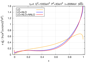
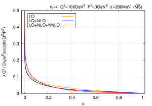
(a)	(b)

Figure 2: Parton distributions in the photon in $\overline{{\rm MS}}$ scheme for $n_{f}=4$, $Q^{2}=100$GeV², $P^{2}=3$GeV² with $\Lambda=0.2$GeV: (a) $xq_{S}^{\gamma}(x,Q^{2},P^{2})|_{\overline{\rm MS}}$ and (b) $xG^{\gamma}(x,Q^{2},P^{2})|_{\overline{\rm MS}}$.

In Fig.2 we plot the parton distributions in $\overline{{\rm MS}}$ scheme in units of $(3n_{f}\langle e^{2}\rangle\alpha/\pi){\rm ln}(Q^{2}/P^{2})$: (a) the singlet quark distribution $xq_{S}^{\gamma}(x,Q^{2},P^{2})|_{\overline{\rm MS}}$ and (b) the gluon distribution $xG^{\gamma}(x,Q^{2},P^{2})|_{\overline{\rm MS}}$. We have taken $n_{f}=4$, $Q^{2}=100{\rm GeV}^{2}$, $P^{2}=3{\rm GeV}^{2}$, and the QCD scale parameter $\Lambda=0.2$GeV. We see that both the (LO+NLO) and (LO+NLO+NNLO) curves show the similar behaviours in almost the whole $x$ region, which means that the NNLO contribution is small. The behaviours of these two curves, however, are quite different from the LO curve. They lie below the LO curve for $0.2<x<0.8$, but diverge as $x\rightarrow 1$. Compared with the quark distribution, the gluon distribution $xG^{\gamma}|_{\overline{\rm MS}}$ is very small in absolute value except in the small-$x$ region. Concerning the nonsinglet quark distribution $xq_{NS}(x,Q^{2},P^{2})|_{\overline{\rm MS}}$, we find that when we take into account the charge factors, such as $\langle e^{2}\rangle=\sum_{i}e_{i}^{2}/n_{f}$ and $\langle e^{4}\rangle=\sum_{i}e_{i}^{4}/n_{f}$, it falls on the singlet quark distribution in almost the whole $x$ region; namely the two “normalised” distributions $x{\widetilde{q}}_{S}^{\gamma}\equiv xq_{S}^{\gamma}/\langle e^{2}\rangle$ and $x{\widetilde{q}}_{NS}^{\gamma}\equiv xq_{NS}^{\gamma}/(\langle e^{4}\rangle-\langle e^{2}\rangle^{2})$ mostly overlap except at the very small $x$ region. This situation is the same in both $\overline{\rm MS}$ and ${\rm DIS}_{\gamma}$ schemes. The rise of the singlet quark distribution near $x=0$ is related to the gluon distribution which grows rapidly as $x\rightarrow 0$.

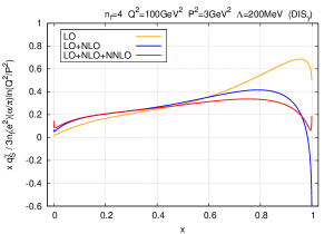
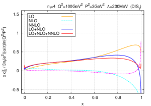
(a)	(b)

Figure 3: (a) Singlet quark distribution $xq_{S}^{\gamma}(x,Q^{2},P^{2})|_{{\rm DIS}_{\gamma}}$ in ${\rm DIS}_{\gamma}$ scheme for $n_{f}=4$, $Q^{2}=100$GeV², $P^{2}=3$GeV² with $\Lambda=0.2$GeV. (b) LO, NLO, and NNLO contributions.

The parton distributions in ${\rm DIS}_{\gamma}$ scheme were analysed up to the NNLO. In Fig.3(a) we plot the singlet quark distribution $xq_{S}^{\gamma}(x,Q^{2},P^{2})|_{{\rm DIS}_{\gamma}}$ in units of $(3n_{f}\langle e^{2}\rangle\alpha/\pi){\rm ln}(Q^{2}/P^{2})$. Again we chose $n_{f}=4$, $Q^{2}=100{\rm GeV}^{2}$, $P^{2}=3{\rm GeV}^{2}$, and $\Lambda=0.2$GeV. The three curves (LO, LO+NLO, LO+NLO+NNLO) rather overlap below $x=0.6$. Absorbing the photonic coefficient function $C_{2}^{\gamma}$ into the quark distributions in ${\rm DIS}_{\gamma}$ scheme has an effect on their large-$x$ behaviours: Unlike the $\overline{\rm MS}$ scheme, the (LO+NLO) curve goes under the LO curve at $x\approx 0.6$ and the difference between the two grows as $x\rightarrow 1$. Adding the NNLO contribution makes the difference bigger at large $x$ except near $x=1$. At very close to $x=1$ the (LO+NLO+NNLO) curve shows a sudden surge. In order to see the details, we plot in Fig.3(b), the NLO and NNLO contributions in ${\rm DIS}_{\gamma}$ scheme. We observe that the NLO contribution is large and negative for $x>0.8$, while the NNLO contribution remains to be very small until very close to $x=1$ and then blows up. The behaviours near $x=1$ of $q_{S}^{\gamma(1)}(x,Q^{2},P^{2})|_{{\rm DIS}_{\gamma}}$ and $q_{S}^{\gamma(2)}(x,Q^{2},P^{2})|_{{\rm DIS}_{\gamma}}$ were discussed in Sec.IV.

Finally, the gluon distribution $xG^{\gamma}(x,Q^{2},P^{2})|_{{\rm DIS}_{\gamma}}$ is the same as $xG^{\gamma}(x,Q^{2},P^{2})|_{\overline{\rm MS}}$.

VI Conclusions

We have analysed the parton distributions in the virtual photon target which are predicted entirely up to the NNLO in perturbative QCD. Parton distributions are dependent on the scheme which is employed to factorise structure functions into parton distributions and coefficient functions. The virtual photon target serves as a good testing ground for examining the behaviours of the parton distributions and their factorisation-scheme dependences. We have studied the quark and gluon distributions in two factorisation schemes, namely, $\overline{\rm MS}$ and ${\rm DIS}_{\gamma}$ schemes.

We see from Figs.2(a) and 3(a) that (LO+NLO) and (LO+NLO+NNLO) curves for the quark distribution $xq_{S}^{\gamma}(x,Q^{2},P^{2})$ show quite different behaviours in two schemes, especially in the large-$x$ region. From the viewpoint of “perturbative stability”, the ${\rm DIS}_{\gamma}$ scheme gives a more appropriate behaviour for $xq_{S}^{\gamma}(x,Q^{2},P^{2})$ than $\overline{\rm MS}$. The gluon distribution $xG^{\gamma}(x,Q^{2},P^{2})$ is the same in both schemes and is predicted to be very small in absolute value except in the small-$x$ region. Finally, we observe that the (LO+NLO+NNLO) curve for $xq_{S}^{\gamma}(x,Q^{2},P^{2})|_{{\rm DIS}_{\gamma}}$ shows a sudden surge at very close to $x=1$. Although the NLO contribution, ${q_{S}^{\gamma(1)}}|_{{\rm DIS}_{\gamma}}$, negatively diverges as ${\rm ln}(1-x)$ for $x\rightarrow 1$, the NNLO ${q_{S}^{\gamma(2)}}|_{{\rm DIS}_{\gamma}}$ diverges positively as $[-{\rm ln}^{3}(1-x)]$. This may hint a necessity of considering the resummation for parton distributions and also for the photon structure function $F_{2}^{\gamma}(x,Q^{2},P^{2})$ itself near $x=1$ Catani .

Appendix A Parameters in $\bm{q}^{\gamma(0)}(t)$, $\bm{q}^{\gamma(1)}(t)$ and $\bm{q}^{\gamma(2)}(t)$

We give here some important information on the parameters which appear in $\bm{q}^{\gamma(0)}(t)$, $\bm{q}^{\gamma(1)}(t)$ and $\bm{q}^{\gamma(2)}(t)$ in Eqs.(33)-(35). They are all calculated in $\overline{\rm MS}$ scheme. We introduce the following quark charge factors:

$$\langle e^{2}\rangle=\frac{1}{n_{f}}\sum^{n_{f}}_{i=1}e^{2}_{i}~{},\qquad\langle e^{4}\rangle=\frac{1}{n_{f}}\sum^{n_{f}}_{i=1}e^{4}_{i}~{},$$

$$f_{S}=3n_{f}\langle e^{2}\rangle~{},\qquad f_{NS}=3n_{f}\Bigl{(}\langle e^{4}\rangle-\langle e^{2}\rangle^{2}\Bigr{)}~{}.$$ (91)

A.1 Initial conditions for parton distributions: ${\widetilde{\bm{A}}}_{n}^{(1)}$ and ${\widetilde{\bm{A}}}_{n}^{(2)}$

The elements of the row vector ${\widetilde{\bm{A}}}_{n}^{(l)}$ are expressed as ${\widetilde{\bm{A}}}_{n}^{(l)}=\Bigl{(}{\widetilde{A}}_{n}^{S(l)},{\widetilde{A}}_{n}^{G(l)},{\widetilde{A}}_{n}^{NS(l)}\Bigr{)}$, with $l=1,2$. Then we have at one-loop level,

$${\widetilde{A}}_{n}^{S(1)}=f_{S}H_{q}^{(1)}(n)~{},\quad{\widetilde{A}}_{n}^{G(1)}=0~{},\quad{\widetilde{A}}_{n}^{NS(1)}=f_{NS}H_{q}^{(1)}(n)~{},$$ (92)

where the explicit expression of $H_{q}^{(1)}(n)$ is given in Eq.(3.30) of Ref.USU . The elements at two-loop level are

$${\widetilde{A}}_{n}^{S(2)}=f_{S}H_{q}^{(2)}(n)~{},\quad{\widetilde{A}}_{n}^{G(2)}=f_{S}H_{G}^{(2)}(n)~{},\quad{\widetilde{A}}_{n}^{NS(2)}=f_{NS}H_{q}^{(2)}(n)~{},$$ (93)

where $H_{q}^{(2)}(n)$ and $H_{G}^{(2)}(n)$ are given in Eqs.(3.39) and (3.42) of Ref.USU , respectively.

A.2 Anomalous dimensions

The one-, two- and three-loop anomalous dimensions for the hadronic sector, ${\widehat{\gamma}}_{n}^{(0)}$, ${\widehat{\gamma}}_{n}^{(1)}$ and ${\widehat{\gamma}}_{n}^{(2)}$ MVV1 ; MVV2 , respectively, are already in literature. The eigenvalues $\lambda_{i}^{n}$ of the one-loop anomalous dimension matrix ${\widehat{\gamma}}_{n}^{(0)}$ and the corresponding projection operators $P_{i}^{n}$ which appeared in Eqs. (31)-(32) are given in Ref.BB . Also the one- and two-loop photonic anomalous dimensions, $\bm{K}_{n}^{(0)}$ and $\bm{K}_{n}^{(1)}$, are already known BB ; FP2 ; GRV . But concerning the three-loop anomalous dimensions $K_{S}^{{(2),n}}$, $K_{G}^{{(2),n}}$ and $K_{NS}^{{(2),n}}$, the exact expressions have not been in literature yet, but approximate ones were given MVV3 . It is remarked there that the precision is within about 0.1% or less. The approximate expressions for $K_{S}^{{(2),n}}$, $K_{NS}^{{(2),n}}$ and $K_{G}^{{(2),n}}$ are

$$K_{S}^{{(2),n}} \approx K_{S\ \rm approx}^{{(2),n}}\equiv-f_{S}~{}2\Bigl{\{}E_{{\rm ns}\gamma}^{\rm approx}(n)+E_{{\rm ps}\gamma}(n)\Bigr{\}}~{},$$

$$K_{G}^{{(2),n}} \approx K_{G\ \rm approx}^{{(2),n}}\equiv-f_{S}~{}2E_{G\gamma}^{\rm approx}(n)~{},$$ (94)

$$K_{NS}^{{(2),n}} \approx K_{NS\ \rm approx}^{{(2),n}}\equiv-f_{NS}~{}2E_{{\rm ns}\gamma}^{\rm approx}(n)~{},$$

where the explicit expressions of $E_{{\rm ns}\gamma}^{\rm approx}(n)$, $E_{{\rm ps}\gamma}(n)$, and $E_{G\gamma}^{\rm approx}(n)$ are given, respectively, in Eqs.(B2), (B4) and (B3) of Ref.USU .

Appendix B Another way to find parton distributions in ${\overline{\rm MS}}$ and ${\rm DIS}_{\gamma}$ scheme

Once we know the expression for the moment sum rule of $F_{2}^{\gamma}(x,Q^{2},P^{2})$ obtained up to the NNLO corrections USU and all the quantities in the expression are the ones calculated in $\overline{\rm MS}$ scheme, then there is an easy way to find the parton distributions in the virtual photon in both ${\overline{\rm MS}}$ and ${{\rm DIS}_{\gamma}}$ schemes up to the NNLO. In the following the equation numbers correspond to those in Ref.USU .

(i) Parton distributions up to the NNLO in ${\overline{\rm MS}}$ scheme
In the moment sum rule of $F_{2}^{\gamma}(x,Q^{2},P^{2})$ given by Eqs.(2.29)-(2.37), we set ${\bm{C}}_{2,n}^{(1)}={\bm{C}}_{2,n}^{(2)}=\bm{0}$ and $C_{2,n}^{\gamma(1)}=C_{2,n}^{\gamma(2)}=0$. In addition, we put $\bm{C}_{2,n}^{(0)}=(1,0,0)^{\rm T}$, then we obtain $q^{\gamma}_{S}(n,Q^{2},P^{2})|_{\overline{\rm MS}}$. Similarly, when we put $\bm{C}_{2,n}^{(0)}=(0,1,0)^{\rm T}$ and $\bm{C}_{2,n}^{(0)}=(0,0,1)^{\rm T}$, we obtain $G^{\gamma}(n,Q^{2},P^{2})|_{\overline{\rm MS}}$ and $q^{\gamma}_{NS}(n,Q^{2},P^{2})|_{\overline{\rm MS}}$ , respectively.

(ii) Parton distributions up to the NNLO in ${\rm DIS}_{\gamma}$ scheme
For the gluon distribution, we have $G^{\gamma}(n,Q^{2},P^{2})|_{{\rm DIS}_{\gamma}}=G^{\gamma}(n,Q^{2},P^{2})|_{\overline{\rm MS}}$ .

• $q^{\gamma}_{NS}(n,Q^{2},P^{2})|_{{\rm DIS}_{\gamma}}$ is obtained as follows:
  Writing  $q^{\gamma}_{NS}|_{{\rm DIS}_{\gamma}}$  as  $q^{\gamma}_{NS}|_{{\rm DIS}_{\gamma}}=q^{\gamma,{(0)}}_{NS}|_{{\rm DIS}_{\gamma}}+q^{\gamma,{(1)}}_{NS}|_{{\rm DIS}_{\gamma}}+q^{\gamma,{(2)}}_{NS}|_{{\rm DIS}_{\gamma}}$,

  • $q^{\gamma,{(0)}}_{NS}|_{{\rm DIS}_{\gamma}}/\Bigl{[}\frac{\alpha}{8\pi\beta_{0}}\Bigr{]}\Bigl{[}\frac{4\pi}{\alpha_{s}(Q^{2})}\Bigr{]}$ is obtained from the term ${\cal{L}}_{NS}^{n}$ in Eq.(2.30), which is the same with $q^{\gamma,{(0)}}_{NS}|_{\overline{MS}}$.

  • $q^{\gamma,{(1)}}_{NS}|_{{\rm DIS}_{\gamma}}/\Bigl{[}\frac{\alpha}{8\pi\beta_{0}}\Bigr{]}$ is obtained from the sum of the terms ${\cal{A}}_{NS}^{n}$, ${\cal{B}}_{NS}^{n}$ and ${\cal{C}}^{n}$ in Eqs.(2.31)-(2.33), where we put, ${\bm{C}}_{2,n}^{(0)}=(0,0,1)^{T}$, ${\bm{C}}_{2,n}^{(1)}=\bm{0}$ and $C_{2,n}^{\gamma(1)}$ is replaced with $C_{2,n}^{\gamma(1)}\times\frac{\langle e^{4}\rangle-\langle e^{2}\rangle^{2}}{\langle e^{4}\rangle}$.

  • $q^{\gamma,{(2)}}_{NS}|_{{\rm DIS}_{\gamma}}/\Bigl{[}\frac{\alpha}{8\pi\beta_{0}}\Bigr{]}\Bigl{[}\frac{\alpha_{s}(Q^{2})}{4\pi}\Bigr{]}$ is obtained from the sum of the terms ${\cal{D}}_{NS}^{n}$, ${\cal{E}}_{NS}^{n}$, ${\cal{F}}_{NS}^{n}$ and ${\cal{G}}^{n}$ in Eqs.(2.34)-(2.37), where we put, ${\bm{C}}_{2,n}^{(0)}=(0,0,1)^{T}$, ${\bm{C}}_{2,n}^{(1)}=\bm{0}$, ${\bm{C}}_{2,n}^{(2)}=\bm{0}$ and $C_{2,n}^{\gamma(2)}$ is replaced with  $\Bigl{(}C_{2,n}^{\gamma(2)}-C_{2,n}^{\gamma(1)}C_{2,n}^{NS(1)}\Bigr{)}\times\frac{\langle e^{4}\rangle-\langle e^{2}\rangle^{2}}{\langle e^{4}\rangle}$.

• $q^{\gamma}_{S}(n,Q^{2},P^{2})|_{{\rm DIS}_{\gamma}}$ is obtained as follows:
  Writing  $q^{\gamma}_{S}|_{{\rm DIS}_{\gamma}}$  as  $q^{\gamma}_{S}|_{{\rm DIS}_{\gamma}}=q^{\gamma,{(0)}}_{S}|_{{\rm DIS}_{\gamma}}+q^{\gamma,{(1)}}_{S}|_{{\rm DIS}_{\gamma}}+q^{\gamma,{(2)}}_{S}|_{{\rm DIS}_{\gamma}}$,

  • $q^{\gamma,{(0)}}_{S}|_{{\rm DIS}_{\gamma}}/\Bigl{[}\frac{\alpha}{8\pi\beta_{0}}\Bigr{]}\Bigl{[}\frac{4\pi}{\alpha_{s}(Q^{2})}\Bigr{]}$ is obtained from the terms $\Bigl{(}{\cal{L}}_{+}^{n}+{\cal{L}}_{-}^{n}\Bigl{)}/\langle e^{2}\rangle$ in Eq.(2.30), which is the same as $q^{\gamma,{(0)}}_{S}|_{\overline{MS}}$. Or we can obtain from the sum of the terms $\sum_{i}{\cal{L}}_{i}^{n}$, where we put, ${\bm{C}}_{2,n}^{(0)}=(1,0,0)^{T}$.

  • $q^{\gamma,{(1)}}_{S}|_{{\rm DIS}_{\gamma}}/\Bigl{[}\frac{\alpha}{8\pi\beta_{0}}\Bigr{]}$ is obtained from the sum of the terms $\sum_{i}{\cal{A}}_{i}^{n}$, $\sum_{i}{\cal{B}}_{i}^{n}$ and ${\cal{C}}^{n}$ in Eqs.(2.31)-(2.33), where we put, ${\bm{C}}_{2,n}^{(0)}=(1,0,0)^{T}$, ${\bm{C}}_{2,n}^{(1)}=\bm{0}$ and $C_{2,n}^{\gamma(1)}$ is replaced with $C_{2,n}^{\gamma(1)}\times\frac{\langle e^{2}\rangle}{\langle e^{4}\rangle}$.

  • $q^{\gamma,{(2)}}_{S}|_{{\rm DIS}_{\gamma}}/\Bigl{[}\frac{\alpha}{8\pi\beta_{0}}\Bigr{]}\Bigl{[}\frac{\alpha_{s}(Q^{2})}{4\pi}\Bigr{]}$ is obtained from the sum of the terms $\sum_{i}{\cal{D}}_{i}^{n}$, $\sum_{i}{\cal{E}}_{i}^{n}$, $\sum_{i}{\cal{F}}_{i}^{n}$ and ${\cal{G}}^{n}$ in Eqs.(2.34)-(2.37), where we put, ${\bm{C}}_{2,n}^{(0)}=(1,0,0)^{T}$, ${\bm{C}}_{2,n}^{(1)}=\bm{0}$, ${\bm{C}}_{2,n}^{(2)}=\bm{0}$ and $C_{2,n}^{\gamma(2)}$ is replaced with  $\Bigl{(}C_{2,n}^{\gamma(2)}-C_{2,n}^{\gamma(1)}C_{2,n}^{NS(1)}\Bigr{)}\times\frac{\langle e^{2}\rangle}{\langle e^{4}\rangle}$.  Note $C_{2,n}^{S(1)}/\langle e^{2}\rangle=C_{2,n}^{NS(1)}$.

References

-
(1)
T.F. Walsh, Phys. Lett. 36B (1971) 121;
S.J. Brodsky, T. Kinoshita and H. Terazawa, Phys. Rev. Lett. 27 (1971) 280. -
(2)
T.F. Walsh and P.M. Zerwas, Phys. Lett. 44B (1973) 195;
R.L. Kingsley, Nucl. Phys. 60 (1973) 45. - (3) N. Christ, B. Hasslacher and A.H. Mueller, Phys. Rev. D6 (1972) 3543.
- (4) E. Witten, Nucl. Phys. B120 (1977) 189.
-
(5)
W.A. Bardeen and A.J. Buras, Phys. Rev. D20 (1979) 166;
Phys. Rev. D21 (1980) 2041, Erratum. - (6) R.J. DeWitt, L.M. Jones, J.D. Sullivan, D.E. Willen and H.W. Wyld, Jr., Phys. Rev. D19 (1979) 2046; Phys. Rev. D20 (1979) 1751, Erratum.
- (7) M. Glück and E. Reya, Phys. Rev. D28 (1983) 2749.
- (8) S. Moch, J.A.M. Vermaseren and A. Vogt, Nucl. Phys. B621 (2002) 413.
- (9) K. Sasaki, Phys. Rev. D22 (1980) 2143; Prog. Theor. Phys. Suppl. 77 (1983) 197.
- (10) M. Stratmann and W. Vogelsang, Phys. Lett. B386 (1996) 370.
-
(11)
M. Glück, E. Reya and C. Sieg, Phys. Lett.
B503 (2001) 285;
Eur. Phys. J. C20 (2001) 271. -
(12)
M. Krawczyk,
AIP Conf. Proc. No.571 (AIP, New York, 2001) and references therein;
M. Krawczyk, A. Zembrzuski and M. Staszel, Phys. Rept. 345 (2001) 265;
R. Nisius, Phys. Rept. 332 (2001) 165; hep-ex/0110078;
M. Klasen, Rev. Mod. Phys. 74 (2002) 1221;
I. Schienbein, Ann. Phys. 301 (2002) 128;
R.M. Godbole, Nucl. Phys. B (Proc. Suppl.) 126 (2004) 414. - (13) T. Uematsu and T.F. Walsh, Phys. Lett. 101B (1981) 263.
- (14) T. Uematsu and T.F. Walsh, Nucl. Phys. B199 (1982) 93.
- (15) G. Rossi, Phys. Rev. D29 (1984) 852.
- (16) M. Drees and R.M. Godbole, Phys. Rev. D50 (1994) 3124.
-
(17)
M. Glück, E. Reya and M. Stratmann, Phys. Rev.
D51 (1995) 3220;
Phys. Rev. D54 (1996) 5515. - (18) M. Fontannaz, Eur. Phys. C 20 (2004) 297.
- (19) K. Sasaki and T. Uematsu, Phys. Rev. D59 (1999) 114011.
- (20) H. Baba, K. Sasaki and T. Uematsu, Phys. Rev. D65 (2002) 114018.
-
(21)
K. Sasaki, T. Ueda and T. Uematsu, Phys. Rev. D73 (2006) 094024;
Nucl. Phys. Proc. Suppl. 157 (2006) 115. - (22) S. Moch, J.A.M. Vermaseren and A. Vogt, Nucl. Phys. B688 (2004) 101.
- (23) A. Vogt, S. Moch and J.A.M. Vermaseren, Nucl. Phys. B691 (2004) 129.
- (24) A. Vogt, S. Moch and J.A.M. Vermaseren, Acta Phys. Polon. B37 (2006) 683; hep-ph/0511112.
- (25) T. Ueda, K. Sasaki and T. Uematsu, Phys. Rev. D75 (2007) 114009.
- (26) Y. Kitadono, K. Sasaki T. Ueda and T. Uematsu, Phys. Rev. D77 (2008) 054019.
- (27) K. Sasaki and T. Uematsu, Phys. Lett. B473 (2000) 309; Eur. Phys. J. C20 (2001) 283.
- (28) T. Ueda, T. Uematsu and K. Sasaki, PoS RADCOR2007 (2007) 036.
- (29) G. Altarelli, Phys. Rep. 81 (1982) 1.
- (30) W. Furmanski and R. Petronzio, Z. Phys. C11 (1982) 293.
- (31) D.R.T. Jones, Nucl. Phys. B75 (1974) 531; W.E. Caswell, Phys. Rev. Lett. 33 (1974) 244.
-
(32)
O.V. Tarasov, A.A. Vladimirov and A.Yu. Zharkov, Phys. Lett. B93 (1980) 429;
S.A. Larin and J.A.M. Vermaseren, Phys. Lett. B303 (1993) 334. - (33) M. Fontannaz and E. Pilon, Phys. Rev. D45 (1992) 382.
- (34) W.-M. Yao et al., Journal of Physics G33 (2006), Eq.(9.5).
- (35) T. Muta, Foundations of quantum chromodynamics (World Scientific, Singapore, 1987).
- (36) W. Celmaster and R. Gonsalves, Phys. Rev. Lett. 42 (1979) 1435.
- (37) W.A. Bardeen, A.J. Buras, D.W. Duke and T. Muta, Phys. Rev. D18 (1978) 3998.
- (38) Y. Matiounine, J. Smith and W.L. van Neerven, Phys. Rev. D57 (1998) 6701.
- (39) M. Glück, E. Reya and A. Vogt, Phys. Rev. D45 (1992) 3986.
- (40) S. Catani, in private communication.