Shot noise in electron transport through a double quantum dot: A master equation approach

Abstract

We study shot noise in tunneling current through a double quantum dot connected to two electric leads. We derive two master equations in the occupation-state basis and the eigenstate basis to describe the electron dynamics. The approach based on the occupation-state basis, despite widely used in many previous studies, is valid only when the interdot coupling strength is much smaller than the energy difference between the two dots. In contrast, the calculations using the eigenstate basis are valid for an arbitrary interdot coupling. We show that the master equation in the occupation-state basis includes only the low-order terms with respect to the interdot coupling compared with the more accurate master equation in the eigenstate basis. Using realistic model parameters, we demonstrate that the predicted currents and shot-noise properties from the two approaches are significantly different when the interdot coupling is not small. Furthermore, properties of the shot noise predicted using the eigenstate basis successfully reproduce qualitative features found in a recent experiment.

I Introduction

Precise control of coherent coupling between quantum states is of great importance in quantum information processing. Recent studies show that artificial two-level systems designed using mesoscopic circuits can be controlled in nanosecond time scales and can also exhibit coherent oscillations between two quantum states (see, e.g., Refs. Nakamura99, ; You05, ; Koppens06, ). A double quantum dot (DQD) provides a useful system to explore coherent effects because interdot hopping intrinsically couples states in two different dots and is tunable via the gate voltage.Petta04 ; Huttel05 A commonly used observable for studying the effects of coherent coupling is the current through the DQD. Recently, shot-noise measurement has recently been demonstrated as another useful tool to study the coherent effects.Barthold07 ; Kiesslich07 Moreover, the shot-noise properties have been predicted to be an indicator of the degree of entanglement between electron statesNeil07 ; Bodoky08 and they are also related to the radiative decay properties of the one-demensional quantum ring exciton.Chen05

Shot noise, i.e., current fluctuations due to the discrete and stochastic nature of electron transport, describes the correlation between electrons transported successively through mesoscopic systems, such as quantum dots (QDs) or molecular devices (for reviews, see Refs. Blanter00, ; Nazarov03, ). In classical transport, the noise is typically Poissonian with a power density $S=2e\langle I\rangle$, where $e$ is the unit charge and $\langle I\rangle$ is the average current. However, either Coulomb interaction or the Pauli’s exclusion principle can induce a negative correlation between successive transport events. This reduces the noise power density so that $S<2e\langle I\rangle$ corresponding to a sub-Poissonian noise.Chen92 In contrast, the interplay between Coulomb interaction and the Pauli’s exclusion principle can also produce a positive correlation between the transport events, i.e., $S>2e\langle I\rangle$. This corresponds to a super-Poissonian noise. The Fano factor $F=S/2e\langle I\rangle$ is usually used to characterize the shot noise, where $F=1$, $F>1$, or $F<1$, respectively, corresponds to the Poissonian, super-Poissonian, or sub-Poissonian noise. Many theoretical works show that super-Poissonian noise of electronBelzig05 ; Sanchez07 ; Sanchez08 or spin, CottetEPL ; Weymann08 ; Ouyang08 ; SanchezNJP and positive cross correlation between different spin statesCottetPRL in QDs can be induced via dynamical channel blockade. Moreover, a super-Poissonian noise in tunneling current caused by dynamical channel blockade has been observed in a system consisting of two electrostatically coupled QDsZhang07 and also a single QDSafonov03 ; Ozarchin07 in recent experiments.

In this work, we study the current and shot-noise in electrons tunneling through a DQD. We apply two different approaches and compare the results. First, we follow many previous investigations (see, e.g., Refs. stoof96, ; Gurvitz96, ; Kiesslich07, ) and derive a master equation for the electron transport based on the occupation-state basis of the DQD. We show that to arrive at this master equation, one needs to assume that the interdot coupling strength is much smaller than the energy difference between the two dots. However, using realistic model parameters for the DQD, only Poissonian or sub-poissonian shot noise is predicted, while super-poissonian noise was also observed in a recent experiment.Barthold07

Alternatively, we derive a more generally applicable master equation in the eigenstate basis of the DQD, which does not require the assumption of a small interdot coupling and is hence valid for any arbitrary interdot coupling strength. The two master equations are formally different in general and are identical only in the limiting case when the interdot coupling is much smaller than the energy difference between the two dots. We show that for small interdot coupling, the properties of the shot noise predicted by the two master equation agree with each other as expected. However, for large interdot coupling, they are significantly different. More importantly, for typical model parameters, the shot noise deduced using the master equation in the eigenstate basis exhibits rich properties including Poissonian, sub-poissonian as well as super-poissonian statistics in good agreement with recent experimental observations (Ref. Barthold07, ). Furthermore, qualitative features of the current and the shot-noise can easily be explained intuitively using the master equation in the eigenstate basis.

The present paper is organized as follows. In Sec. II, we introduce the model for a DQD connected to two electric leads. A phonon bath that affects the dynamics of the DQD is also considered. Two master equations for the electron dynamics in the DQD are derived in both the occupation-state basis and the eigenstate basis. In Sec. III and Sec. IV, we study, respectively, the properties of the current through the DQD and the associated shot noise. Results based on the two master equations are compared. In Sec. V, we discuss the relation between the two master equations. A brief conclusion is presented in Sec. VI. Finally, Appendixes A and B give detailed derivations of the master equations in both the occupation-state basis and the eigenstate basis.

II Time evolution of the reduced density matrix of a double quantum dot

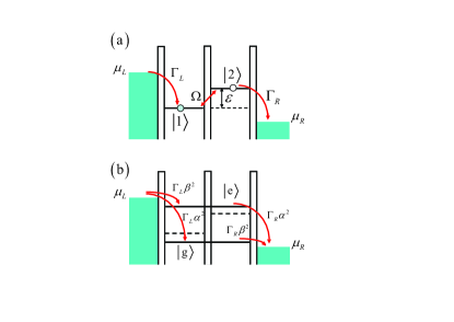
Figure 1: (Color online) Schematic diagram of an electron transported through a DQD connected to two electric leads via tunneling barriers. (a) Considering DQD electron states in the occupation-state basis, the electron tunnels sequentially from the left lead to the right lead via first the left dot and then the right dot. (b) Considering the eigenstate basis, the electron is transport via either the ground-state channel or and the excited-state channel. The effective tunneling rates from the left lead to the ground state and the excited state are $\Gamma_{L}\alpha^{2}$ and $\Gamma_{L}\beta^{2}$, while those from the ground state and the excited state to the right lead are $\Gamma_{R}\beta^{2}$ and $\Gamma_{R}\alpha^{2}$.

The schematic diagram of a DQD connected to two electrodes by tunneling barriers is shown in Fig. 1. The voltage across the DQD is biased so that the chemical potential of the left electrode $\mu_{L}$ is higher than that of the right electrode $\mu_{R}$. Thus, an electron can tunnel from the left electrode to the right one via the DQD. We assume that the DQD is in the Coulomb regime (with both strong intra- and interdot Coulomb repulsions), so that at most a single electron is allowed in the DQD. In the occupation representation, the electron basis states are the vacuum state $|0\rangle$, the state with one electron in the left dot $|1\rangle$, and the state with one electron in the right dot $|2\rangle$.

The Hamiltonian of the whole system reads (taking $\hbar=1$)

$$H_{\rm{tot}}\!=\!H_{\rm{leads}}+H_{\rm{DQD}}+H_{\rm{T}}+H_{\rm{ph}}+H_{\rm{ep}}.$$ (1)

The first two terms $H_{\rm{leads}}$ and $H_{\rm{DQD}}$ are respectively the Hamiltonians of the two electrodes and the DQD, and are given by

$$H_{\rm{leads}} = \sum_{\alpha k}\omega_{\alpha k}c_{\alpha k}^{\dagger}c_{\alpha k},$$ (2)

$$H_{\rm{DQD}} = \frac{\varepsilon}{2}\sigma_{z}+\Omega\sigma_{x},$$ (3)

where $c_{\alpha k\sigma}^{\dagger}$ ($c_{\alpha k\sigma}$) is the creation (annihilation) operator of an electron with momentum $k$ in the electrode $\alpha$ $(\alpha=l,r)$; $\sigma_{z}=a_{2}^{\dagger}a_{2}-a_{1}^{\dagger}a_{1}$ and $\sigma_{x}=a_{2}^{\dagger}a_{1}+~{}a_{1}^{\dagger}a_{2}$ are the Pauli matrices, with $a_{1}^{\dagger}$ ($a_{2}^{\dagger}$) being the electron creation operator in the left (right) dot of the DQD. In Eq. (3), the first term $\varepsilon\sigma_{z}/2$, with $\varepsilon=\varepsilon_{2}-\varepsilon_{1}$ denoting the energy difference between the two dots, gives the Hamiltonian of the two uncoupled quantum dots, while the second term $\Omega\sigma_{x}$ characterizes the interdot hopping. The tunneling coupling between the DQD and the electrodes is described by

$$H_{\rm{T}}=\sum_{k}(\Omega_{lk}\;a_{1}^{\dagger}\,c_{lk}+\Omega_{rk}\;a_{2}^{\dagger}\,\Upsilon_{r}\,c_{rk}+\rm{H.c.}),$$ (4)

where $\Omega_{lk(rk)}$ is the tunneling strength between the QD and the left (right) electrode. The operators $\Upsilon_{r}$ ($\Upsilon_{r}^{\dagger}$) decreases (increases) the number of electrons having tunneled into the right lead (via the barrier between the DQD and the right lead).Doiron07 These counting operators allow one to keep track of the tunneling process during the evolution of the DQD. Below we focus on current and shot noise in electron tunneling through the right tunneling barrier, so only the related counting operators ($\Upsilon_{r}$ and $\Upsilon_{r}^{\dagger}$) are introduced in the tunneling Hamiltonian (4).

Also, we consider the effects of the phonon-bath environment on the evolution of the DQD. The Hamiltonian of this phonon bath is

$$H_{\rm{ph}}=\sum_{q}\omega_{q}b_{q}^{\dagger}b_{q},$$ (5)

with $b_{q}^{\dagger}$ ($b_{q}$) creating (annihilating) a phonon with frequency $\omega_{q}$. The electron-phonon interaction is given by

$$H_{\rm{ep}}=\sigma_{x}\sum_{q}\lambda_{q}(b_{q}^{\dagger}+b_{q}),$$ (6)

where $\lambda_{q}$ is the electron-phonon coupling strength.

The evolution of the whole system is described by the von Neumann equation for the density matrix $\rho_{R}$ of the whole system:

$$\dot{\rho}_{R}(t)=-i[\,H_{\rm{tot}},~{}\rho_{R}(t)\,].$$ (7)

Here we are interested in the time evolution of the DQD and treat both the electric leads and the phonon bath as the total outside environment. We will hence derive the master equation of the reduced density matrix $\rho_{d}$ of the DQD: $\rho_{d}\equiv\,{\rm Tr}_{E}\{\rho_{R}\}$, where ${\rm Tr}_{E}\{\cdots\}$ denotes the trace over the degrees of freedom of both the electric leads and the phonon bath. In our calculations, we adopt the interaction picture based on the free Hamiltonian

$$H_{0}=H_{\rm{leads}}+H_{\rm{ph}}+H_{\rm{DQD}},$$ (8)

and the interaction Hamiltonian becomes

$$H_{\rm int}(t) = H_{\rm T}(t)+H_{\rm ep}(t),$$ (9)

where operators in the interaction and the Schrodinger pictures are related by $A(t)=e^{iH_{0}t}Ae^{-iH_{0}t}$ for any operator $A$.

After tracing over the degrees of freedom of both the electrodes and the phonon bath, one obtains the master equation for the reduced density matrix $\rho_{d}^{I}$ of the DQD in the interaction picture asBlum

$$\dot{\rho}^{I}_{d}(t) = -i\,{\rm Tr}_{E}[\,H_{\rm int}(t),~{}\rho_{d}(0)\rho_{E}(0)\,]$$

$$-{\rm Tr}_{E}\int_{0}^{t}dt^{\prime}[\,H_{\rm int}(t),\,[\,H_{\rm int}(t^{\prime}),\,\rho^{I}_{d}(t^{\prime})\rho_{E}(0)]\;],$$

where $\rho_{E}$ is the density matrix of the outside environment. Because the trace of a single unpaired creation or annihilation operator over the lead or the phonon bath is zero, e.g., ${\rm Tr}_{E}\{c_{lk}\rho_{E}\}=0$, the first term in Eq. (LABEL:ME-1) vanishes. Within the Born-Markov approximation, we have

$$\dot{\rho}^{I}_{d}(t)=-{\rm Tr}_{E}\int_{0}^{t}dt^{\prime}[\,H_{\rm int}(t),\,[\,H_{\rm int}(t^{\prime}),\,\rho^{I}_{d}(t)\rho_{E}(0)]\;],$$

(11)

Here the Born approximation amounts to the use of the second-order perturbation theory with respect to the interaction Hamiltonian $H_{\rm int}$, while the Markov approximation assumes that the correlation times of the outside environment (both the electric leads and the phonon bath) are much shorter than the typical quantum-state evolution time of the DQD.

Since the left lead, the right lead and the phonon bath are completely independent of each other, the density matrix of the outside environment $\rho_{E}$ can be written as a tensor product of density matrices that describe the subsystems, i.e., $\rho_{E}=\rho_{L}\rho_{R}\rho_{\rm ph}$, where $\rho_{L}$, $\rho_{R}$ and $\rho_{\rm ph}$ are, respectively, the density matrices of the left lead, the right lead and the phonon bath. Therefore, the trace of the integrand in Eq. (11) can be expressed as:

$${\rm Tr}_{E}[\,H_{\rm int}(t),\;[\,H_{\rm int}(t^{\prime}),\,\rho^{I}_{d}(t)\rho_{E}]\;]$$ (12)

$$\!=\! \!\sum_{\alpha=l,r}{\rm Tr_{\alpha}}[\,H_{\rm T}(t),\,[\,H_{\rm T}(t^{\prime}),\rho^{I}_{d}(t)\rho_{\rm\alpha}]\;]$$

$$+\,{\rm Tr_{ph}}\,[\,H_{\rm ep}(t),\,[\,H_{\rm ep}(t^{\prime}),\;\rho^{I}_{d}(t)\rho_{\rm ph}]\;].$$

Equation (11) can thus be written as a sum of two corresponding parts:

$$\dot{\rho}_{d}^{I}(t)\! \!=\! \!\mathcal{L}_{\rm T}\rho_{d}^{I}(t)+\mathcal{L}_{\rm ph}\rho_{d}^{I}(t).$$ (13)

Here, the dissipative part due to the electric leads is given by

$$\mathcal{L}_{\rm T}\rho_{d}^{I}(t)\! \!=\! \!-\sum_{\alpha=l,r}{\rm Tr}_{\alpha}\int\limits_{0}^{t}dt^{\prime}\big{[}\,H_{\rm T}(t)H_{\rm T}(t^{\prime})\rho_{d}^{I}(t)\,\rho_{\rm leads}$$ (14)

$$-H_{\rm T}(t)\rho_{d}^{I}(t)\,\rho_{\rm leads}H_{\rm T}(t^{\prime})+{\rm H.c.}\,\big{]},$$

where $\rho_{\rm leads}=\rho_{L}\rho_{R}$ is the density matrix of the two electric leads. The dissipative part caused by the phonon bath is

$$\mathcal{L}_{\rm ph}\rho_{d}^{I}(t)\! \!=\! \!-{\rm Tr}_{\rm ph}\int\limits_{0}^{t}dt^{\prime}\big{[}\,H_{\rm ep}(t)H_{\rm ep}(t^{\prime})\rho_{d}^{I}(t)\,\rho_{\rm ph}$$ (15)

$$-H_{\rm ep}(t)\rho_{d}^{I}(t)\,\rho_{\rm ph}H_{\rm ep}(t^{\prime})+{\rm H.c.}\,\big{]}.$$

From Eqs. (13)–(15), one can derive the master equation for the $n$-resolved reduced density matrix $\rho^{(n)}_{d}(t)$ of the DQD, where $\rho^{(n)}_{d}(t)\equiv\langle n|\rho_{d}(t)|n\rangle$ and $n$ is the number of electrons that have arrived at the right lead at time $t$. Below we derive two versions of the master equation in both the occupation-state basis and the eigenstate basis and then use them independently to study the current and shot-noise properties of the DQD.

II.1 Master equation in the occupation-state basis

The master equation of the DQD in the occupation-state basis was previously used to study the current propertiesstoof96 ; Gurvitz96 and shot-noise propertiesKiesslich07 ; Weymann08 ; SanchezNJP ; Sanchez08 of electrons tunneling through the DQD. The occupation-state basis is defined by the states $|0\rangle$, $|1\rangle$, and $|2\rangle$, which correspond to the states of an empty DQD, one electron in the left dot, and one electron in the right dot, respectively. In the interaction picture defined by the free Hamiltonian $H_{0}$ in Eq. (8), the unperturbed evolution operator $U_{0}(t)=e^{iH_{0}t}$ is difficult to calculate in the occupation-state basis in the presence of interdot coupling. One hence split $H_{0}$ into two parts:

$$H_{0}=H_{1}+H_{\Omega},$$ (16)

where

$$H_{1} = H_{\rm{leads}}+H_{\rm{ph}}+\frac{\varepsilon}{2}\sigma_{z},$$ (17)

$$H_{\Omega} = \Omega\sigma_{x}.$$ (18)

Following previously worksGoan01 ; Korotkov99 on deriving master equations in the occupation-state basis, we assume that the interdot couping $\Omega$ is small and satisfies $\Omega\ll|\varepsilon_{2}-\varepsilon_{1}|$, we have $H_{0}\simeq H_{1}$. The evolution operator can then be approximated as

$$e^{iH_{0}t}\simeq e^{iH_{1}t}.$$ (19)

With this approximation, one easily obtains

$$H_{\rm T}(t)\! \!\approx\! \!\sum_{k}[\,\Omega_{lk}\;a_{1}^{\dagger}\,c_{lk}e^{-i(\omega_{lk}-\omega_{1})t}$$ (20)

$$+\;\Omega_{rk}\,\Upsilon_{r}\,a_{2}^{\dagger}\,c_{rk}e^{-i(\omega_{rk}-\omega_{2})t}+\rm{H.c.}\,],$$

and

$$H_{\rm ep}(t)\! \!\approx\! \!(\sigma_{+}e^{i\varepsilon t}+\sigma_{-}e^{-i\varepsilon t})\sum_{q}\lambda_{q}(b_{q}^{\dagger}e^{i\omega_{q}t}+b_{q}e^{-i\omega_{q}t}),$$

where $\omega_{1,2}\equiv\mp\varepsilon/2$. Here $\sigma_{+}\!=\!a_{2}^{\dagger}a_{1}$ and $\sigma_{-}\!=\!\sigma_{+}^{\dagger}$ are the raising and lowing operators in the occupation-state basis.

We now consider the nonequilibrium case with a large bias voltage across the DQD, so that all energy levels of the DQD lie within the bias window, as shown in Figs. 1(a) and 1(b). Substituting Eqs. (20) and (LABEL:H-sb(t)) into Eqs. (13)–(15), taking the trace over the degrees of freedom of both the two electrodes and the phonon bath, and converting the obtained equation to the Schrödinger picture, one arrives at the master equation in the occupation-state basis for a weak interdot coupling $\Omega\ll|\varepsilon_{2}-\varepsilon_{1}|$ (see Appendix A):

$$\dot{\rho}_{d}(t)\! \!=\! \!-i[\,H_{\rm DQD},\,\rho_{d}]+\frac{\Gamma_{L}}{2}\mathcal{D}[a_{1}^{\dagger}]\rho_{d}+\frac{\Gamma_{R}}{2}\mathcal{D}[\Upsilon_{r}^{\dagger}a_{2}]\rho_{d}$$ (22)

$$+\frac{\gamma_{1}}{2}\mathcal{D}[\sigma_{-}]\rho_{d}+\frac{\gamma_{2}}{2}\mathcal{D}[\sigma_{+}]\rho_{d},$$

where $\Gamma_{L(R)}=2\pi\rho_{lk(rk)}\Omega_{lk(rk)}^{2}$ is the electron tunneling rate through the left (right) tunneling barrier. Here, the electron density of states $\rho_{\alpha k}$ at lead $\alpha$ ($\alpha=l,r$) and the tunneling strength $\Omega_{\alpha k}$ are assumed to be energy-independent. The notation $\mathcal{D}$ acting on any operator $A$ is defined as

$$\mathcal{D}[A]\rho=2A\rho A^{\dagger}-[A^{\dagger}A\rho+\rho A^{\dagger}A].$$ (23)

The dissipation rates induced by the electron-phonon interaction are

$$\gamma_{1} = 2\pi\big{\{}{{J}\left(\varepsilon\right)\left[{n\left(\varepsilon\right)+1}\right]+{J}\left({-\varepsilon}\right)n\left({-\varepsilon}\right)}\big{\}},$$

$$\gamma_{2} = 2\pi\big{\{}{{J}\left({-\varepsilon}\right)\left[{n\left({-\varepsilon}\right)+1}\right]+{J}\left(\varepsilon\right)n\left(\varepsilon\right)}\big{\}},$$ (24)

where

$${J}(\omega)=\sum\limits_{q}{\lambda_{q}^{2}\;\delta\left({\omega-\omega_{q}}\right)},$$ (25)

is the bath spectral density and $n\left(\omega\right)\!=\![{{\exp\left({\omega/k_{B}T}\right)-1}}]^{-1}$ is the average phonon number at temperature $T$. Using Eq. (22) and the relations:Doiron07

$$\langle n|\Upsilon_{r}^{\dagger}\Upsilon_{r}\rho_{d}|n\rangle = \rho_{d}^{(n)},$$

$$\langle n|\Upsilon_{r}\Upsilon_{r}^{\dagger}\rho_{d}|n\rangle = \rho_{d}^{(n)},$$

$$\langle n|\Upsilon_{r}^{\dagger}\rho_{d}\Upsilon_{r}|n\rangle = \rho_{d}^{(n-1)},$$

$$\langle n|\Upsilon_{r}\rho_{d}\Upsilon_{r}^{\dagger}|n\rangle = \rho_{d}^{(n+1)},$$ (26)

one obtains the equation of motion for each density matrix element:

$$\dot{\rho}_{\rm 00}^{(n)}(t)\! \!=\! \!-\Gamma_{L}\rho_{\rm 00}^{(n)}+\Gamma_{R}\rho_{22}^{(n-1)},$$

$$\dot{\rho}_{11}^{(n)}\left(t\right)\! \!=\! \!\Gamma_{L}\rho_{00}^{(n)}+i\,\Omega\left({\rho_{12}^{(n)}-\rho_{21}^{(n)}}\right)+\gamma_{1}\rho_{22}^{(n)}-\gamma_{2}\rho_{11}^{(n)},$$

$$\dot{\rho}_{22}^{(n)}\left(t\right)\! \!=\! \!-\Gamma_{R}\rho_{22}^{(n)}-i\,\Omega\left({\rho_{12}^{(n)}-\rho_{21}^{(n)}}\right)-\gamma_{1}\rho_{22}^{(n)}+\gamma_{2}\rho_{11}^{(n)},$$

$$\dot{\rho}_{12}^{(n)}(t)\! \!=\! \!i\varepsilon\rho_{12}^{(n)}+i\,\Omega\left({\rho_{11}^{(n)}-\rho_{22}^{(n)}}\right)-\frac{{\Gamma_{R}+\gamma_{1}+\gamma_{2}}}{2}\rho_{12}^{(n)}.$$

Then, the $i$th diagonal matrix element $\rho_{ii}=\sum_{n}\rho_{ii}^{(n)}$ ($i=0,1$, or $2$) gives the occupation probability of the state $|i\rangle$. The off-diagonal matrix element $\rho_{12}(t)=\sum_{n}\rho_{12}^{(n)}$ describes the coherence between states $|1\rangle$ and $|2\rangle$, and $\rho_{21}(t)=\rho_{12}^{\ast}(t)$. This master equation was used in many previous studies, e.g., Refs. stoof96, and Gurvitz96, .

The physical meaning of the master equation can be understood as follows. Take the equation for $\rho_{11}^{(n)}$ in Eq. (LABEL:EOM-elements-O) for example. The first term on the right-hand side describes the process of an electron tunneling from the left lead to the left dot with rate $\Gamma_{L}$. The second term represents the coherent coupling between states $|1\rangle$ and $|2\rangle$ due to the interdot coupling. The third term describes the phonon-induced relaxation process from state $|2\rangle$ to $|1\rangle$ with rate $\gamma_{1}$. Finally, the fourth term describes the inverse process with rate $\gamma_{2}$.

II.2 Master equation in the eigenstate basis

As explained above, the master equation in the occupation-state basis is only valid for a weak interdot coupling. To extend the results to an arbitrary interdot coupling $\Omega$, we now derive the master equation in the eigenstate basis of the DQD. The result is valid for any arbitrary interdot coupling strength.

Diagonalizing the Hamiltonian of the DQD [Eq. (3)], one has

$$H_{\rm DQD}=\frac{\Omega_{0}}{2}\,(\,|e\rangle\langle e|-|g\rangle\langle g|\,)=\frac{\Omega_{0}}{2}\,\sigma_{z}^{(e)},$$ (28)

where $\Omega_{0}=\sqrt{\varepsilon^{2}+4\,\Omega^{2}}$ is the energy splitting of the two eigenstates of the DQD given by

$$|e\rangle = \sin\frac{\theta}{2}\,|1\rangle+\cos{\frac{\theta}{2}}\,|2\rangle,$$

$$|g\rangle = \cos\frac{\theta}{2}\,|1\rangle-\sin{\frac{\theta}{2}}\,|2\rangle,$$ (29)

with $\tan\theta=2\Omega/\varepsilon$. The eigenstates and the occupation states are related by

$$\left|1\right\rangle = \cos\frac{\theta}{2}\,\left|g\right\rangle+\,\sin\frac{\theta}{2}\,\left|e\right\rangle,$$

$$\left|2\right\rangle = -\sin\frac{\theta}{2}\,\left|g\right\rangle+\cos\frac{\theta}{2}\,\left|e\right\rangle.$$ (30)

With these relations, the tunneling Hamiltonian [Eq. (4)] and the electron-phonon interaction [Eq. (6)] can be written, in the eigenstate basis, as

$$H_{\rm{T}}\! \!=\! \!\sum_{k}\bigg{[}\Omega_{lk}\;{\big{(}\,{\cos\frac{\theta}{2}\,a_{g}^{\dagger}+\,\sin\frac{\theta}{2}\,a_{e}^{\dagger}}\,\big{)}}\,c_{lk}$$

$$+\,\Omega_{rk}\;{\big{(}\,{-\sin\frac{\theta}{2}\,a_{g}^{\dagger}+\,\cos\frac{\theta}{2}\,a_{e}^{\dagger}}\,\big{)}}\,\Upsilon_{r}\,c_{rk}+\rm{H.c.}\bigg{]},$$

$$H_{\rm ep}\! \!=\! \!\left[{\sin\theta\,\,\sigma_{z}^{(e)}+\cos\theta\,\,\sigma_{x}^{(e)}}\right]\sum\limits_{q}{\lambda_{q}\left({b_{q}^{\dagger}+b_{q}}\right)}.$$

In the interaction picture based on the free Hamiltonian $H_{0}$ given by Eq. (8), they become

$$H_{\rm{T}}(t)\! \!=\! \!\sum_{k}\big{\{}\Omega_{lk}{\big{(}\,{\cos\frac{\theta}{2}\,a_{g}^{\dagger}e^{i\omega_{g}t}+\sin\frac{\theta}{2}\,a_{e}^{\dagger}e^{i\omega_{e}t}}\,\big{)}}c_{lk}$$ (32)

$$e^{-i\omega_{lk}t}+\Omega_{rk}{\big{[}{-\sin\frac{\theta}{2}a_{g}^{\dagger}e^{i\omega_{g}t}+\,\cos\frac{\theta}{2}\,a_{e}^{\dagger}}e^{i\omega_{e}t}\,\big{]}}$$

$$\times\Upsilon_{r}c_{rk}e^{-i\omega_{rk}t}+\rm{H.c.}\big{\}},$$

$$H_{\rm ep}(t)\! \!=\! \!\left[{\sin\theta\,\,\sigma_{z}^{(e)}+\cos\theta\,\,(\sigma_{+}^{(e)}e^{i\Omega_{0}t}+\sigma_{-}^{(e)}e^{-i\Omega_{0}t})}\right]$$ (33)

$$\times\sum\limits_{q}{\lambda_{q}\left({b_{q}^{\dagger}e^{i\omega_{q}t}+b_{q}e^{-i\omega_{q}t}}\right)},$$

where $\omega_{g,e}=\mp\Omega_{0}/2$. Here $\sigma_{-}^{(e)}=a_{g}a_{e}^{\dagger}$ and $\sigma_{+}^{(e)}=(\sigma_{-}^{(e)})^{\dagger}$ are the lowering and raising operators in the eigenstate basis.

Now, one can evaluate Eqs. (13)–(15) using Eqs. (32) and (33). After converting the result to the Schrödinger picture, one obtains the master equation in the eigenstate basis which holds for any arbitrary interdot coupling $\Omega$ (see Appendix B):

$$\dot{\rho}_{d}(t)\! \!=\! \!-i[\,H_{\rm DQD},~{}\rho_{d}(t)\,]+\frac{\Gamma_{L}}{2}\alpha^{2}\mathcal{D}\,[a_{g}^{\dagger}]\,\rho_{d}$$

$$\!+\frac{\Gamma_{L}}{2}\beta^{2}\mathcal{D}\,[a_{e}^{\dagger}]\,\rho_{d}+\frac{\Gamma_{R}}{2}\beta^{2}\mathcal{D}\,[a_{g}\Upsilon_{r}^{\dagger}]\rho_{d}$$

$$+\frac{\Gamma_{R}}{2}\alpha^{2}\mathcal{D}[a_{e}\Upsilon_{r}^{\dagger}]\rho_{d}+\frac{\lambda_{1}}{2}\mathcal{D}[\sigma_{-}^{(e)}]\rho_{d}+\frac{\lambda_{2}}{2}[\sigma_{+}^{(e)}]\rho_{d},$$

where

$$\alpha\equiv\cos{\frac{\theta}{2}}=\sqrt{\frac{\Omega_{0}+\varepsilon}{2\Omega_{0}}},~{}~{}~{}\beta\equiv\sin{\frac{\theta}{2}}=\sqrt{\frac{\Omega_{0}-\varepsilon}{2\Omega_{0}}},$$ (35)

and

$$\lambda_{1} = \gamma_{0}\cos^{2}{\theta}\,[\,n(\Omega_{0})+1\,],$$

$$\lambda_{2} = \gamma_{0}\cos^{2}{\theta}\,n(\Omega_{0}).\,$$ (36)

with $\gamma_{0}=2\pi{J}(\Omega_{0})$. Using Eq. (LABEL:ME-E), the $n$-resolved equation of motion for each density matrix element can be written as

$$\dot{\rho}_{00}^{(n)}(t)\! \!=\! \!-\Gamma_{L}\rho_{00}^{(n)}+\Gamma_{R}\beta^{2}\rho_{gg}^{(n-1)}+\Gamma_{R}\alpha^{2}\rho_{ee}^{(n-1)},$$

$$\dot{\rho}_{gg}^{(n)}(t)\! \!=\! \!\Gamma_{L}\alpha^{2}\rho_{00}^{(n)}-\Gamma_{R}\beta^{2}\rho_{gg}^{(n)}+\lambda_{1}\rho_{ee}^{(n)}-\lambda_{2}\rho_{gg}^{(n)},$$

$$\dot{\rho}_{ee}^{(n)}(t)\! \!=\! \!\Gamma_{L}\beta^{2}\rho_{00}^{(n)}-\Gamma_{R}\alpha^{2}\rho_{ee}^{(n)}-\lambda_{1}\rho_{ee}^{(n)}+\lambda_{2}\rho_{gg}^{(n)}.$$

It follows from Eq. (LABEL:EOM-elements-E) that the effective tunneling rate from the left lead to the ground (excited) state $|g\rangle$ ($|e\rangle$) is $\Gamma_{L}\alpha^{2}$ ($\Gamma_{L}\beta^{2}$), while the effective tunneling rate from the ground (excited) state to the right lead is $\Gamma_{R}\beta^{2}$ ($\Gamma_{R}\alpha^{2}$) [see Fig. 1(b)]. We emphasize that these results derived in the eigenstate basis are valid for any arbitrary interdot coupling.

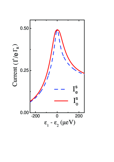
Figure 2: (Color online) Stationary current $I^{s}$ through the DQD as a function of the energy difference $\varepsilon_{1}-\varepsilon_{2}$ calculated using the occupation-state basis ($I^{s}=I_{\rm o}^{s}$) and the eigenstate basis ($I^{s}=I_{\rm e}^{s}$) for a $large$ interdot coupling $\Omega=32~{}\mu$eV. We have taken $\Gamma_{L}=100~{}\mu$eV, $\Gamma_{R}=2.5~{}\mu$eV, $\gamma_{0}=0.6~{}\mu$eV, and $T=2~{}$K.

III current through the double quantum dot

To compare the master equations in Eqs. (LABEL:EOM-elements-O) and  (LABEL:EOM-elements-E) derived, respectively, in the occupation-state basis and the eigenstate basis, we first apply them to study the tunneling current through the DQD. In the next section, the associated shot noise will also be studied. The current $I(t)$ through the DQD at time $t$ is given by

$$I(t)=e\frac{dN(t)}{dt}=e\sum_{n,i}n\dot{\rho}_{ii}^{(n)}(t),$$ (38)

where $N(t)$ is the number of electrons that have tunneled into the right lead. Here, $i$ is summed over all basis states of the basis used.

Denoting results based on the occupation-state basis and the eigenstate basis by “o” and “e”, values of the current $I_{\rm o}(t)$ and $I_{\rm e}(t)$ calculated using Eqs. (LABEL:EOM-elements-O) and (LABEL:EOM-elements-E) are

$$I_{\rm o}(t)\! =\!e\,\Gamma_{R}\,\rho_{22}(t),$$ (39a)

$$I_{\rm e}(t)\! =\!e\,[\,\Gamma_{R}\beta^{2}\rho_{gg}(t)+\Gamma_{R}\alpha^{2}\rho_{ee}(t)\,],$$ (39b)

At steady-state with $\dot{\rho}_{ii}(t)=0$, calculated values $I_{\rm o}^{s}$ and $I_{\rm e}^{s}$ of the stationary current are

$$I_{\rm o}^{s}\! \!=\!\frac{e\Gamma_{L}\Gamma_{R}}{\Lambda}\times\big{\{}\,\gamma_{2}\;[\,4\varepsilon^{2}+(\gamma_{1}+\gamma_{2}+\Gamma_{R})^{2}\,]$$

$$+\;4\Omega^{2}(\gamma_{1}+\gamma_{2}+\Gamma_{R})\big{\}},$$ (40a)

$$I_{\rm e}^{s}\! \!=\!\frac{e{\Gamma_{L}\Gamma_{R}\left[{\beta^{2}\lambda_{1}+\alpha^{2}\left({\lambda_{2}+\beta^{2}\Gamma_{R}}\right)}\right]}}{\Xi},$$ (40b)

where

$$\Lambda\! \!=4\Omega^{2}\Gamma_{R}\left({2\Gamma_{L}+\Gamma_{R}}\right)+\left({\gamma_{2}+\Gamma_{L}}\right)\Gamma_{R}\left({4\varepsilon^{2}+\Gamma_{R}^{2}}\right)$$

$$+\left({\gamma_{1}+\gamma_{2}}\right)\bigg{[}4\Gamma_{L}(\varepsilon^{2}+2\Omega^{2})+4\Omega^{2}\Gamma_{R}$$

$$+\Gamma_{L}(\gamma_{1}+\gamma_{2})^{2}+\,\Gamma_{R}(\gamma_{2}+3\Gamma_{L})(\gamma_{1}+\gamma_{2})$$

$$+\Gamma_{R}^{2}\,(2\gamma_{2}+3\Gamma_{L})\bigg{]},$$ (41a)

$$\Xi\! \!=\lambda_{2}\left(\Gamma_{L}+\alpha^{2}\Gamma_{R}\right)+\lambda_{1}\left(\Gamma_{L}+\beta^{2}\Gamma_{R}\right)$$

$$+\Gamma_{R}\left[\left(\alpha^{4}+\beta^{4}\right)\Gamma_{L}+\alpha^{2}\beta^{2}\Gamma_{R}\right].$$ (41b)

Figure 2 shows the calculated values $I_{\rm o}^{s}$ and $I_{\rm e}^{s}$ of the stationary current through the DQD. We choose a typical interdot coupling $\Omega=32~{}\mu$eV, which is experimentally accessible.Gustavsson07 For both $I_{\rm o}^{s}$ and $I_{\rm e}^{s}$ at the resonant tunneling point characterized by $\varepsilon_{1}-\varepsilon_{2}=0$, the current reaches its maximum. Moreover, it can be seen that the current is asymmetric around the maximum point. This asymmetry was also observed in a recent experiment by Barthold et al..Barthold07 It is due to dissipations induced by the phonon bath, as we will now demonstrate. In the absence of electron-phonon coupling, we have $\gamma_{1}=\gamma_{2}=0$ and $\lambda_{1}=\lambda_{2}=0$, so that Eqs. (40a) and (40b) reduces to

$$I_{\rm o}^{s}\! =\!\frac{{4\,e\,\Omega^{2}\Gamma_{L}\Gamma_{R}}}{{4\Omega^{2}\left({2\Gamma_{L}+\Gamma_{R}}\right)+4\varepsilon^{2}\Gamma_{L}+\Gamma_{L}\Gamma_{R}^{2}}},$$ (42a)

$$I_{\rm e}^{s}\! =\!\frac{{4\,e\,\Omega^{2}\Gamma_{L}\Gamma_{R}}}{{4\Omega^{2}\left({2\Gamma_{L}+\Gamma_{R}}\right)+4\varepsilon^{2}\Gamma_{L}}},$$ (42b)

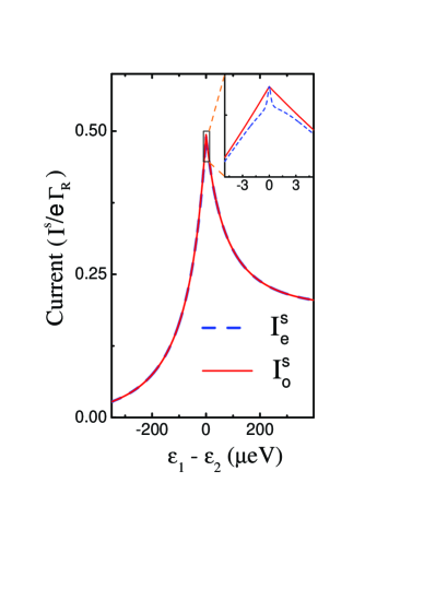
Figure 3: (Color online)  Stationary current $I^{s}$ as a function of $\varepsilon_{1}-\varepsilon_{2}$ calculated using the occupation-state basis ($I^{s}=I_{\rm o}^{s}$) and the eigenstate basis ($I^{s}=I_{\rm e}^{s}$) for a $small$ interdot coupling $\Omega=1~{}\mu$eV. Inset: The enlarged diagram of the stationary current $I^{s}$ in the region with $|\varepsilon_{2}-\varepsilon_{1}|$ comparable to $\Omega$.

where Eq. (42a) agrees with the result from previous studies,Gurvitz02 ; Kiesslich07 in which the occupation-state basis was also used. From Eqs. (42a) and (42b), it is clear that the current as predicted using either the occupation-state basis or the eigenstate basis is symmetric about the current peak at $\varepsilon_{1}=\varepsilon_{2}$. This reveals that this asymmetry of the current is due to the coupling of the DQD to the phonon bath.

As shown in Sec. II, the master equation derived in the occupation-state basis is only valid in the limit of a weak interdot coupling, i.e., $\Omega\ll|\varepsilon_{2}-\varepsilon_{1}|$, while that in the eigenstate basis is valid for any arbitrary interdot coupling. Figure 3 plots the values of the stationary current calculated in the two bases for a small interdot coupling ($\Omega=1~{}\mu$eV). As expected, when the interdot coupling $\Omega$ is much smaller than the energy difference $|\varepsilon_{2}-\varepsilon_{1}|$ of the two dots, the stationary-state current calculated in the occupation-state basis agrees very well with that in the eigenstate basis, as is evident from Fig. 3. However, when the interdot coupling is comparable to the energy difference, the stationary currents in the occupation-state basis deviates drastically from the stationary current in the eigenstate basis (see Fig. 2). This deviation can also be revealed in Fig. 3 in the narrow region with $|\varepsilon_{2}-\varepsilon_{1}|\sim\Omega$ ($=1\mu eV$) (see the inset of Fig. 3). These clearly show the inaccuracy of the current and hence the master equation in the occupation-state basis at large $\Omega$. In this case, one must use the master equation derived in the eigenstate basis.

IV shot noise

To calculate the shot noise in the tunneling current through the DQD, it is particularly useful to define a generating function for an electron counting variable $s$ (see Refs. Sanchez07, ; Ouyang08, and DongPRL, ):

$$G(t,s)=\sum_{n}s^{n}\rho^{(n)}(t).$$ (43)

This generation function obeys the equation of motion

$$\dot{G}(t,s)=M(s)G(t,s),$$ (44)

where $M(s)$ is a transition matrix that can be calculated using the master equation [Eq. (22) or (LABEL:ME-E)]. Statistics on the number of transported electrons $n$ can be determined from the derivatives of the generating function:

$$\frac{\partial^{p}{\rm{tr}}G(t,1)}{\partial s^{p}}=\big{\langle}\prod_{i=1}^{p}(n-i+1)\big{\rangle}.$$ (45)

In particular, the mean of $n$ is

$$\langle n\rangle=\frac{\partial{\rm{tr}}G(t,1)}{\partial s},$$ (46)

and the variance reads

$$\sigma_{n}^{2}=\langle n^{2}\rangle-\langle n\rangle^{2}=\frac{\partial^{2}{\rm{tr}}G(t,1)}{\partial s^{2}}+\langle n\rangle-\langle n\rangle^{2}.$$ (47)

Applying the Laplace transform to the equation of motion, Eq. (44), of the generating function, one has

$$\tilde{G}(z,s)=(z-M)^{-1}G(0,s).$$ (48)

Because of the incoherent long-time stability of the considered system, the real parts of all the non-zero poles of $\tilde{G}(z,s)$ are negative. Therefore, the long-time behavior is determined by the pole $z_{0}$ closest to zero, i.e., $G(t,s)\!\sim\!g(s)e^{z_{0}t}$. By the Taylor expansion of the pole

$$z_{0}=\sum_{m>0}c_{m}(s-1)^{m},$$ (49)

one obtains

$$\langle n\rangle=\frac{\partial{g(1)}}{\partial s}+c_{1}t,$$

$$\sigma_{n}^{2}=\frac{\partial^{2}g(1)}{\partial{s^{2}}}-\bigg{(}\frac{\partial g(1)}{\partial s}\bigg{)}^{2}+(c_{1}+2c_{2})t.$$

(50)

In particular, the Fano factor of the shot noise is given by

$$F=1+2\;\frac{c\,_{2}}{c\,_{1}},$$ (51)

where $F>1$ $(F<1)$ indicates super(sub)-Poissonian noise, compared to $F=1$ for classical Poissonian noise.

We first consider results based on the occupation-state basis. To calculate the Fano factor, we can show, using Eqs. (LABEL:EOM-elements-O) and (48), that the pole $z_{0}$ follows

$$a_{1}\left({s-1}\right)+a_{2}z_{0}+a_{3}\left({s-1}\right)z_{0}$$

$$+\;a_{4}z_{0}^{2}+a_{5}z_{0}^{2}\left({s-1}\right)+a_{6}z_{0}^{3}+a_{7}z_{0}^{4}+z_{0}^{5}=0,$$

(52)

with

$$a_{1}\! \!=\! \!-\frac{1}{4}\Gamma_{L}\Gamma_{R}\big{\{}4\varepsilon^{2}\gamma_{2}+(\gamma_{1}+\gamma_{2}+\Gamma_{R})$$

$$\times[4\Omega^{2}+\gamma_{2}(\gamma_{1}+\gamma_{2}+\Gamma_{R})]\big{\}},$$

$$a_{2}\! \!=\! \!\frac{1}{4}\bigg{\{}\Gamma_{L}(\gamma_{1}+\gamma_{2})[4(\varepsilon^{2}+2\Omega^{2})+(\gamma_{1}+\gamma_{2})^{2}]$$

$$+\big{\{}(\gamma_{1}+\gamma_{2})[4\Omega^{2}+\gamma_{2}(\gamma_{1}+\gamma_{2})]$$

$$+\Gamma_{L}[8\Omega^{2}+3(\gamma_{1}+\gamma_{2})^{2}]+4\varepsilon^{2}(\gamma_{2}+\Gamma_{L})\big{\}}\Gamma_{R}$$

$$+[4\Omega^{2}+(\gamma_{1}+\gamma_{2})(2\gamma_{2}+3\Gamma_{L})]\Gamma_{R}^{2}+(\gamma_{2}+\Gamma_{L})\Gamma_{R}^{3}\bigg{\}},$$

$$a_{3}\! \!=\! \!-\Gamma_{L}\Gamma_{R}[2\Omega^{2}+\gamma_{2}(\gamma_{1}+\gamma_{2}+\Gamma_{R})],$$

$$a_{4}\! \!=\! \!\frac{1}{4}\bigg{\{}\gamma_{1}^{3}+\gamma_{2}^{3}+4(\varepsilon^{2}+4\Omega^{2})(\Gamma_{L}+\Gamma_{R})+5\Gamma_{L}\Gamma_{R}^{2}$$ (53)

$$+\Gamma_{R}^{3}+\gamma_{1}^{2}(3\gamma_{2}+5\Gamma_{L}+3\Gamma_{R})+\gamma_{2}^{2}(5\Gamma_{L}+7\Gamma_{R})$$

$$+\gamma_{2}(4\varepsilon^{2}+8\Omega^{2}+10\Gamma_{L}\Gamma_{R}+7\Gamma_{R}^{2})$$

$$+\gamma_{1}\big{[}4\varepsilon^{2}+8\Omega^{2}+3\gamma_{2}^{2}+10\Gamma_{L}\Gamma_{R}+3\Gamma_{R}^{2}$$

$$+10\gamma_{2}(\Gamma_{L}+\Gamma_{R})\big{]}\bigg{\}}.$$

The expressions for $a_{5}$, $a_{6}$ and $a_{7}$ are not involved in further calculations and are not reported here.

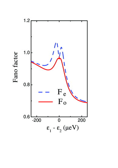
Figure 4: (Color online) Fano factor $F$ as a function of $\varepsilon_{1}-\varepsilon_{2}$ calculated using the occupation-state basis ($F=F_{\rm o}$) and the eigenstate basis ($F=F_{\rm e}$) for a $large$ interdot coupling $\Omega=32~{}\mu$eV.

Using also Eqs. (49) and (51), the Fano factor $F_{\rm o}$ in the occupation-state basis is found to be

$$F_{\rm o}=1+2\times\frac{a_{1}\,a_{4}\,-\,a_{2}\,a_{3}}{a_{2}^{2}}.$$ (54)

Without any phonon dissipation effect, i.e., $\gamma_{1}=\gamma_{2}=0$, the Fano factor becomes

$$F_{\rm o}\!=\!1-\frac{{8\Omega^{2}\Gamma_{L}\left[{4\varepsilon^{2}\left({\Gamma_{R}-\Gamma_{L}}\right)+3\Gamma_{L}\Gamma_{R}^{2}+\Gamma_{R}^{3}+8\Omega^{2}\Gamma_{R}}\right]}}{{\left[{\Gamma_{L}\Gamma_{R}^{2}+4\Gamma_{L}\varepsilon^{2}+4\Omega^{2}\left({\Gamma_{R}+2\Gamma_{L}}\right)}\right]^{2}}},$$ (55)

which is identical to the previous resultsGurvitz02 ; Brandes05 obtained in the occupation-state basis. For a super-Poissonian noise, one has $F_{\rm o}>1$. From Eq. (55), it follows that

$$4\varepsilon^{2}(\Gamma_{L}-\Gamma_{R})>3\Gamma_{L}\Gamma_{R}^{2}+\Gamma_{R}^{3}+8\Omega^{2}\Gamma_{R}.$$ (56)

Alternatively, using the eigenstate basis, one can obtain from Eqs. (LABEL:EOM-elements-E) and (48) the following equation for the pole $z_{0}$:

$$b_{1}(s-1)+b_{2}z_{0}+b_{3}z_{0}+b_{4}z_{0}+z^{3}=0,$$ (57)

where

$$b_{1}\! \!=\! \!-\Gamma_{L}\Gamma_{R}\,[\alpha^{2}(\lambda_{2}+\beta^{2}\Gamma_{R})+\beta^{2}\lambda_{1}\,],$$

$$b_{2}\! \!=\! \!\lambda_{1}(\Gamma_{L}+\Gamma_{R}\beta^{2})+\lambda_{2}(\Gamma_{L}+\alpha^{2}\Gamma_{R})$$

$$+\,\Gamma_{R}[\,\Gamma_{L}(\alpha^{2}+\beta^{2}-2\alpha^{2}\beta^{2})+\alpha^{2}\beta^{2}\Gamma_{R}\,],$$

$$b_{3}\! \!=\! \!-2\alpha^{2}\beta^{2}\Gamma_{L}\Gamma_{R},$$

$$b_{4}\! \!=\! \!\lambda_{1}+\lambda_{2}+\Gamma_{L}+\Gamma_{R}.$$ (58)

In contrast to Eq. (52), only four coefficients $b_{i}$ ($i=1$ to $4$) appear in Eq. (57). From an equation for $F_{\rm e}$ analogous to Eq. (54) for $F_{\rm o}$, we get

$$F_{e} = 1+\frac{2\Gamma_{L}\Gamma_{R}}{\Xi^{2}}\times\big{\{}2\alpha^{2}\beta^{2}\,\Xi\,-(\lambda_{1}+\lambda_{2}+\Gamma_{L}+\Gamma_{R})$$ (59)

$$\times[\,\beta^{2}\lambda_{1}+\alpha^{2}\lambda_{2}+\alpha^{2}\beta^{2}\Gamma_{R}\,]\,\big{\}},$$

where $\Xi$ is given in Eq. (41b). Without phonon dissipation, i.e., $\lambda_{1}=\lambda_{2}=0$, one obtains after substituting Eq. (35) into Eq. (59),

$$F_{\rm e}=1-\frac{{8\Omega^{2}\Gamma_{L}}\times\left\{{4\varepsilon^{2}\left({\Gamma_{R}-\Gamma_{L}}\right)+8\Omega^{2}\Gamma_{R}}\right\}}{{\left[\,{4\varepsilon^{2}\Gamma_{L}+4\Omega^{2}\left({2\Gamma_{L}+\Gamma_{R}}\right)}\,\right]^{2}}}.$$ (60)

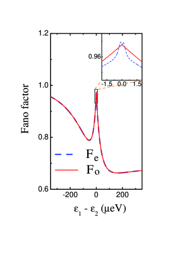
Figure 5: (Color online) Fano factor $F$ as a function of $\varepsilon_{1}-\varepsilon_{2}$ calculated using the occupation-state basis ($F=F_{\rm o}$) and the eigenstate basis ($F=F_{\rm e}$) for a $small$ interdot coupling $\Omega=1~{}\mu$eV. Inset: The enlarged diagram of the Fano factor $F$ in the region with $|\varepsilon_{1}-\varepsilon_{2}|$ comparable to $\Omega$.

Figure 4 presents both of the calculated Fano factors $F_{\rm o}$ and $F_{\rm e}$ of the shot noise based on the occupation-state basis and eigenstate basis, respectively. At the resonant tunneling point, i.e., $\varepsilon_{1}=\varepsilon_{2}$, both approaches predict that the shot noise is sub-Poissonian. For $F_{\rm o}$, in the absence of phonon-induced dissipation, a super-Poissonian noise can be obtained with the condition Eq. (56). Due to the effects of dissipation, $F_{\rm o}$ has only sub-Poissonian noise for the whole parameter range investigated here. In contrast, $F_{\rm e}$ has much richer behaviors of super-Poissonian, sub-Poissonian, and Poissonian noise correlations, depending on the energy difference $\varepsilon_{1}-\varepsilon_{2}$. Moreover, $F_{\rm e}$, but not $F_{\rm o}$, exhibits a double-peak structure and an asymmetry around the dip at $\varepsilon_{1}=\varepsilon_{2}$. These features were also observed in a recent experiment (see Ref. Barthold07, ).

The double peak in the Fano factor predicted using the eigenstate basis can be intuitively understood as follows. The electrons can tunnel from the DQD to the right lead via two channels, namely, the ground-state channel and the excited-state channel. At the resonant tunneling point ($\varepsilon_{1}=\varepsilon_{2}$), the tunnel rate through the ground-state channel is the same as that through the excited-state channel. This results in a sub-Poissonian shot noise.Sanchez07 When $\varepsilon_{1}<\varepsilon_{2}$, one has $\Gamma_{g}<\Gamma_{e}$, and the electron transport through the ground-state channel blocks that through the excited-state channel. This dynamical channel blockade leads to a super-Possionian shot noise.Belzig05 However, when $\varepsilon_{2}-\varepsilon_{1}\gg\Omega$, $\Gamma_{g}$ becomes zero and the electron can only tunnel through the DQD via the excited-state channel. This single-channel tunneling gives rise to a sub-Poissonian shot noise,Chen92 as shown in Fig. 4. Similarly, when $\varepsilon_{1}>\varepsilon_{2}$, one has $\Gamma_{g}>\Gamma_{e}$ and the tunneling through the excited-state channel blocks that through the ground-state channel. The noise is super-Poissonian for a small energy difference $\varepsilon_{1}-\varepsilon_{2}$, due to the dynamical channel blockade. When $\varepsilon_{1}-\varepsilon_{2}\gg\Omega$, $\Gamma_{e}$ becomes zero and the electron can only tunnel through the DQD via the ground-state channel. This single-channel tunneling also gives rise to a sub-Poissonian noise.

The asymmetry of the shot noise is caused by the relaxation process induced by the electron-phonon interaction. When $\varepsilon_{1}<\varepsilon_{2}$, we have $\Gamma_{g}<\Gamma_{e}$ and the relaxation process from the excited state to the ground state enhances the dynamical channel blockade. However, when $\varepsilon_{1}>\varepsilon_{2}$, one has $\Gamma_{g}>\Gamma_{e}$ and the relaxation process from the excited state to the ground state suppresses the dynamical channel blockade. The asymmetry of the Fano factor hence follows [see Fig. 4].

We have shown using Fig. 4 that for a large interdot coupling, e.g., $\Omega=32~{}\mu$eV, the Fano factor in the occupation-state basis deviates drastically from the Fano factor in the eigenstate basis. This verifies that the small interdot coupling approximation in deriving the master equation in the occupation-state basis is invalid. Instead, the master equation in the eigenstate basis should be used. As a further consistency check, Fig. 5 shows the Fano factor of the shot noise for a small interdot coupling strength ($\Omega=1~{}\mu$eV). As expected, the calculated Fano factors using both basis agrees with each other except for the small region with $|\varepsilon_{2}-\varepsilon_{1}|\sim\Omega$; in this small region, the results in the two cases are different because the condition $|\varepsilon_{2}-\varepsilon_{1}|\gg\Omega$ is not satisfied (see the inset of Fig. 5).

V Correction terms for the Occupation-State Master equation

In this section, we derive a controlled series expansion for the scattering term in the quantum master equation with respect to the interdot coupling strength. This provides a concise quantitative description of the approximation used in the occupation-state approach. In general, it can also allow one to derive correction terms, either to improve the results based on the occupation-state approach or to estimate the resulting error.

The master equations in both approaches are derived from Eq. (LABEL:ME-1) in the interaction picture. To study the difference between the two approaches, we first transform Eq. (LABEL:ME-1) back to the Schrödinger picture and get

$$\dot{\rho}_{d}(t)\! \!=\! \!-i{\rm Tr}_{E}[H_{0},\rho_{d}(t)\rho_{E}(0)]$$

$$-{\rm Tr}_{E}\int\limits^{\infty}_{0}d\tau[H_{\rm int},e^{-iH_{0}\tau}[\,H_{\rm int},\rho_{d}(t)\rho_{E}(0)]e^{iH_{0}\tau}],$$

where we have put $\tau=t-t^{\prime}$ and assumed $t\gg 0$. It can further be written in the more compact form Weiss

$$\dot{\rho}_{d}(t)\! = \!{\rm Tr}_{E}[\mathcal{L}_{0}\rho_{d}(t)\rho_{E}]$$ (62)

$$+{\rm Tr}_{E}\int\limits^{\infty}_{0}d\tau\mathcal{L}_{\rm int}e^{\mathcal{L}_{0}\tau}\mathcal{L}_{\rm int}\rho_{d}(t)\rho_{E},$$

where $\mathcal{L}_{0}$ and $\mathcal{L}_{\rm int}$ are the Liouville operators for the Hamiltonians $H_{0}$ and $H_{\rm int}$, respectively. The Liouville operator $\mathcal{L}_{0}$, for instances, is defined by $\mathcal{L}_{0}A=-i[H_{0},A]$ for any operator $A$. We have also used $e^{\mathcal{L}_{0}\tau}A=e^{-iH_{0}\tau}Ae^{iH_{0}\tau}$ which follows directly from the Baker-Hausdorff lemma.Sakurai

In the eigenstate basis, $e^{\mathcal{L}_{0}\tau}$ in Eq. (62) is treated exactly. However, in the occupation-state basis, it can only be approximated. To illustrate this approximation and study the associated correction terms, we note that $\mathcal{L}_{0}=\mathcal{L}_{1}+\mathcal{L}_{\Omega}$ because of Eq. (16) and derive the Dyson series

$$e^{\mathcal{L}_{0}\tau}=e^{\mathcal{L}_{1}\tau}+\int_{0}^{\tau}d\tau^{\prime}e^{\mathcal{L}_{1}(\tau-\tau^{\prime})}\mathcal{L}_{\Omega}e^{\mathcal{L}_{1}\tau^{\prime}}+\cdots,$$ (63)

where $\mathcal{L}_{1}$ and $\mathcal{L}_{\Omega}$ denote the Liouville operators for $H_{1}$ and $H_{\Omega}$, respectively. Equation (62) then becomes

$$\dot{\rho}_{d}(t)={\rm Tr}_{E}[\mathcal{L}_{0}\rho_{d}(t)\rho_{E}]$$

$$+{\rm Tr}_{E}\int_{0}^{\infty}d\tau\mathcal{L}_{\rm int}e^{\mathcal{L}_{1}\tau}\mathcal{L}_{\rm int}\rho_{d}(t)\rho_{E}$$

$$+{\rm Tr}_{E}\int\limits_{0}^{\infty}d\tau\!\int\limits_{0}^{\tau}\!d\tau^{\prime}\mathcal{L}_{\rm int}e^{\mathcal{L}_{1}(\tau-\tau^{\prime})}\mathcal{L}_{\Omega}e^{\mathcal{L}_{1}\tau^{\prime}}\mathcal{L}_{\rm int}\rho_{d}(t)\rho_{E}$$

$$+\cdots.$$ (64)

Taking only the first two terms, we arrive at the approximate master equation used in the occupational-state basis, which is identical to Eq. (62) with $e^{\mathcal{L}_{0}\tau}$ approximated by $e^{\mathcal{L}_{1}\tau}$. The third term in Eq. (64) is then the leading correction term for the master equation in the occupational-state basis. It consists of terms of order $\mathcal{O}(\Omega\Omega_{lk}^{2})$ or $\mathcal{O}(\Omega\lambda_{q}^{2})$. Expressions for higher order correction terms in the occupational-state approach can similarly be calculated.

For our DQD problem, the correction terms can also be obtained by a direct comparison with the eigenstate basis result. Without the lose of generality, we assume $\varepsilon_{2}-\varepsilon_{1}>0$ in the following discussion. In the small interdot-coupling limit with $\Omega\ll|\varepsilon_{2}-\varepsilon_{1}|$, $\alpha$ and $\beta$ defined in Eq. (35) reduce approximately to

$$\alpha\approx 1,~{}~{}\beta\approx\eta,$$ (65)

where $\eta=\Omega/\varepsilon\ll 1$. The transformation between the two bases given in Eq. (29) can be approximated by

$$|g\rangle\! \!\approx\! \!|1\rangle-\eta\,|2\rangle,$$

$$|e\rangle\! \!\approx\! \!\eta\,|1\rangle+|2\rangle.$$ (66)

Substituting Eq. (66) into the master equation in the eigenstate basis [Eq. (LABEL:ME-E)], and keeping terms only up to first order in $\eta$, one has

$$\dot{\rho}_{d}(t)\approx-i\big{[}\,H_{\rm DQD},~{}\rho_{d}(t)\,\big{]}+\frac{\Gamma_{L}}{2}\mathcal{D}[a_{1}^{\dagger}]\rho_{d}$$

$$+\frac{\Gamma_{R}}{2}\mathcal{D}[a_{2}\Upsilon_{r}^{\dagger}]\rho_{d}+\frac{\gamma_{1}}{2}\mathcal{D}[a_{2}^{\dagger}a_{1}]\rho+\frac{\gamma_{2}}{2}\mathcal{D}[a_{1}^{\dagger}a_{2}]\rho_{d}$$

$$-\Gamma_{L}\eta[a_{2}^{\dagger}\rho_{d}a_{1}+a_{1}^{\dagger}\rho_{d}a_{2}]$$

$$+\frac{\Gamma_{R}}{2}\eta\big{[}2a_{1}\Upsilon_{r}^{\dagger}\rho_{d}\Upsilon_{r}a_{2}^{\dagger}+2a_{2}\Upsilon_{r}^{\dagger}\rho_{d}\Upsilon_{r}a_{1}^{\dagger}-\sigma_{x}\rho_{d}-\rho_{d}\sigma_{x}\big{]}$$

$$-\gamma_{1}\eta\big{[}a_{1}^{\dagger}a_{2}\rho_{d}\sigma_{z}+\sigma_{z}\rho_{d}a_{2}^{\dagger}a_{1}\big{]}-\frac{\gamma_{1}-\gamma_{2}}{2}\eta[\sigma_{x}\rho_{d}+\rho_{d}\sigma_{x}]$$

$$-\gamma_{2}\eta\big{[}a_{2}^{\dagger}a_{1}\rho_{d}\sigma_{z}+\sigma_{z}\rho_{d}a_{1}^{\dagger}a_{2}\big{]}.$$ (67)

Indeed, when $\eta\!=\!0$, this equation reduces to the approximate master equation in the occupation-state basis [Eq. (22)]. The terms proportional to $\eta$ are the leading correction terms of the order $\mathcal{O}(\Omega\Omega_{lk}^{2})$ or $\mathcal{O}(\Omega\lambda_{q}^{2})$ as expected.

VI Conclusion

In summary, we have derived two master equations in both the occupation-state basis and the eigenstate basis to describe the dynamics of the DQD. We show that the master equation in the occupation-state basis is only valid for a small interdot coupling, while the master equation in the eigenstate basis is valid for an arbitrary interdot coupling. To demonstrate the difference between these two master equations, we focus on the current and shot-noise properties in electron tunneling through the DQD. When the interdot coupling is much smaller than the energy difference between the two dots, the current and shot noise in the occupation-state basis are very close to those in the eigenstate basis. For a large interdot coupling, however, the properties derived in the occupation-state basis deviate drastically from those in the eigenstate basis. This reveals that the master equation in the occupation-state basis is not accurate for the case of a large interdot coupling and in this case the master equation in the eigenstate basis should be used. Also, we show that the shot-noise properties predicted using the eigenstate basis can successfully reproduce the features found in a recent experiment.Barthold07 Moreover, we have discussed the relation between these two master equations and show explicitly that the master equation in the occupation-state basis only includes low order terms with respect to the interdot coupling, compared with the master equation derived in the eigenstate basis.

Appendix A Derivation of master equation in occupation-state basis

In this appendix, we give further details of the derivation of the master equation in the occupation-state basis outlined in Sec. IIA. We first evaluate $\mathcal{L}_{\rm T}\rho_{d}^{I}(t)$. Using the expression for $H_{T}(t)$ in Eq. (20), the first term in Eq. (14) becomes

$$-\int_{0}^{\infty}d\tau\bigg{\{}\sum\limits_{lk}{\Omega_{lk}^{2}a_{1}a_{1}^{\dagger}\rho_{d}^{I}\left(t\right)e^{i\left({\omega_{lk}-\omega_{1}}\right)\tau}\left\langle{c_{lk}^{\dagger}c_{lk}}\right\rangle}$$

$$+\sum\limits_{lk}{\Omega_{lk}^{2}a_{1}^{\dagger}a_{1}\rho_{d}^{I}\left(t\right)e^{-i\left({\omega_{lk}-\omega_{1}}\right)\tau}\left\langle{c_{lk}c_{lk}^{\dagger}}\right\rangle}$$

$$+\sum\limits_{rk}{\Omega_{rk}^{2}a_{2}a_{2}^{\dagger}\Upsilon_{r}^{\dagger}\Upsilon_{r}\rho_{d}^{I}\left(t\right)e^{i\left({\omega_{rk}-\omega_{2}}\right)\tau}\left\langle{c_{rk}^{\dagger}c_{rk}}\right\rangle}$$

$$+\sum\limits_{rk}{\Omega_{rk}^{2}a_{2}^{\dagger}a_{2}\Upsilon_{r}\Upsilon_{r}^{\dagger}\rho_{d}^{I}\left(t\right)e^{-i\left({\omega_{rk}-\omega_{2}}\right)\tau}\left\langle{c_{rk}c_{rk}^{\dagger}}\right\rangle}\bigg{\}},$$

(68)

where $\tau=t-t^{\prime}$. When the electron density of states in an electric lead is dense, each sum in Eq. (68) can be replaced by an integral. After some algebra, we obtain

$$-\sum_{\alpha=l,r}{\rm Tr}_{\alpha}\int\limits_{0}^{t}dt^{\prime}\big{[}\,H_{\rm T}(t)H_{\rm T}(t^{\prime})\rho_{d}^{I}(t)\,\rho_{\rm leads}(0)$$

$$=-\frac{{\Gamma_{L}}}{2}\left[{a_{1}a_{1}^{\dagger}\rho_{d}^{I}f_{l}\left({\omega_{1}}\right)+a_{1}^{\dagger}a_{1}\rho_{d}^{I}\bar{f}_{l}\left({\omega_{1}}\right)}\right]$$

$$-\frac{{\Gamma_{R}}}{2}\left[{a_{2}a_{2}^{\dagger}\Upsilon_{r}^{\dagger}\Upsilon_{r}\rho_{d}^{I}f_{r}\left({\omega_{2}}\right)+a_{2}^{\dagger}a_{2}\Upsilon_{r}\Upsilon_{r}^{\dagger}\rho_{d}^{I}\bar{f}_{r}\left({\omega_{2}}\right)}\right],$$

(69)

where $\Gamma_{L,R}=2\pi\rho_{lr,rk}\Omega_{lk,rk}^{2}$ is the electron tunneling rate through the left (right) barrier. Here

$$f_{\alpha}(\omega_{i})=\frac{1}{1+e^{(\omega_{i}-\mu_{\alpha})/k_{B}T}},$$ (70)

is the Fermi-Dirac distribution with $\mu_{\alpha}$ being the chemical potential of lead $\alpha$ and $\bar{f}_{\alpha}(\omega_{i})=1-f_{\alpha}(\omega_{i})$. Note that, in deriving Eq. (69), we have used the relations

$$\langle c_{\alpha k}^{\dagger}c_{\alpha k}\rangle=f_{\alpha}(\omega_{\alpha k}),~{}~{}~{}\langle c_{\alpha k}c_{\alpha k}^{\dagger}\rangle=1-f_{\alpha}(\omega_{\alpha k}),$$ (71)

and

$$\int_{0}^{\infty}d\tau\;e^{\pm i(\omega_{\alpha k}-\omega_{i})\tau}\approx\pi\delta(\omega_{\alpha k}-\omega_{i}).$$ (72)

Similarly, the second term in Eq. (14) can be calculated as

$$\sum_{\alpha=l,r}{\rm Tr}_{\alpha}\int\limits_{0}^{t}dt^{\prime}\big{[}\,H_{\rm T}(t)\rho_{d}^{I}(t)\,\rho_{\rm leads}(0)H_{\rm T}(t^{\prime})\,\big{]}$$

$$=\frac{{\Gamma_{L}}}{2}\left[{a_{1}\rho_{d}^{I}a_{1}^{\dagger}\bar{f}_{l}\left({\omega_{1}}\right)+a_{1}^{\dagger}\rho_{d}^{I}a_{1}f_{l}\left({\omega_{1}}\right)}\right]$$

$$+\frac{{\Gamma_{R}}}{2}\left[{a_{2}\Upsilon_{r}^{\dagger}\rho_{d}^{I}\Upsilon_{r}a_{2}^{\dagger}\bar{f}_{r}\left({\omega_{2}}\right)+a_{2}^{\dagger}\Upsilon_{r}\rho_{d}^{I}\Upsilon_{r}^{\dagger}a_{2}f_{r}\left({\omega_{2}}\right)}\right].$$

(73)

Substituting Eqs. (69) and (73) into Eq. (14), one obtains

$$\mathcal{L}_{\rm T}\rho_{d}^{I}(t)=\frac{{\Gamma_{L}}}{2}\mathcal{D}[a_{1}]\rho_{d}^{I}(t)\bar{f}_{l}(\omega_{1})+\frac{{\Gamma_{L}}}{2}\mathcal{D}[a_{1}^{\dagger}]\rho_{d}^{I}(t)f_{l}(\omega_{1})$$

$$+\frac{{\Gamma_{R}}}{2}\mathcal{D}[a_{2}\Upsilon_{r}^{\dagger}]\rho_{d}^{I}(t)\bar{f}_{r}\left({\omega_{2}}\right)+\frac{{\Gamma_{R}}}{2}\mathcal{D}\left[{a_{2}^{\dagger}\Upsilon_{r}}\right]\rho_{d}^{I}(t)f_{r}\left({\omega_{2}}\right),$$

(74)

where $\mathcal{D}$ (acting on any operator $A$) is defined by

$$\mathcal{D}[A]\rho=2A\rho A^{\dagger}-A^{\dagger}A\rho-\rho A^{\dagger}A,$$ (75)

for any given operator $A$.

Following similar procedures, substituting the value of $H_{\rm ep}(t)$ in Eq. (LABEL:H-sb(t)) into Eq. (15) and after some algebra, one obtains

$$\mathcal{L}_{\rm ph}\rho_{d}^{I}(t)\! \!=\! \!\frac{{\gamma_{2}}}{2}\mathcal{D}\left[{\sigma_{+}}\right]\rho_{d}^{I}(t)+\frac{{\gamma_{1}}}{2}\mathcal{D}\left[{\sigma_{-}}\right]\rho_{d}^{I}(t),$$ (76)

with

$$\gamma_{1}\! \!=\! \!2\pi\left\{{J\left(\varepsilon\right)\left[{n\left(\varepsilon\right)+1}\right]+J\left({-\varepsilon}\right)n\left({-\varepsilon}\right)}\right\},$$

$${\rm{}}\gamma_{2}\! \!=\! \!2\pi\left\{{J\left({-\varepsilon}\right)\left[{n\left({-\varepsilon}\right)+1}\right]+J\left(\varepsilon\right)n\left(\varepsilon\right)}\right\},$$ (77)

where

$${J}\left(\omega\right)=\sum\limits_{q}{\lambda_{q}^{2}\delta\left({\omega-\omega_{q}}\right)},$$ (78)

is the bath spectra density and

$$n\left(\varepsilon\right)=\frac{1}{{\exp\left({\varepsilon/k_{B}T}\right)-1}},$$ (79)

is the Bose-Einstein distribution.

With $\mathcal{L}_{\rm T}\rho_{d}^{I}(t)$ and $\mathcal{L}_{\rm ph}\rho_{d}^{I}(t)$ given by Eq. (74) and Eq. (76), the master equation, Eq. (13), for the reduced density matrix of the DQD in the interaction picture is found to be

$$\dot{\rho}_{d}^{I}(t) = \frac{{\Gamma_{L}}}{2}\mathcal{D}[a_{1}]\rho_{d}^{I}\bar{f}_{l}(\omega_{1})+\frac{{\Gamma_{L}}}{2}\mathcal{D}[a_{1}^{\dagger}]\rho_{d}^{I}f_{l}(\omega_{1})$$ (80)

$$+\frac{{\Gamma_{R}}}{2}\mathcal{D}[a_{2}\Upsilon_{r}^{\dagger}]\rho_{d}^{I}\bar{f}_{r}\left({\omega_{2}}\right)+\frac{{\Gamma_{R}}}{2}\mathcal{D}\left[{a_{2}^{\dagger}\Upsilon_{r}}\right]\rho_{d}^{I}f_{r}\left({\omega_{2}}\right)$$

$$+\frac{{\gamma_{2}}}{2}\mathcal{D}\left[{\sigma_{+}}\right]\rho_{d}^{I}+\frac{{\gamma_{1}}}{2}\mathcal{D}\left[{\sigma_{-}}\right]\rho_{d}^{I}.$$

Next, we assume both a large bias voltage across the DQD (i.e., $\mu_{L}>\omega_{1},~{}\omega_{2}>\mu_{R}$) and a very low temperature, so that $f_{l}({\omega_{1}})=1,\,f_{r}(\omega_{2})=0$. After converting the resulting equation into the Schrödinger picture using the free evolution operator $e^{-iH_{0}t}$ or its approximate in Eq. (19), we finally have

$$\dot{\rho}_{d}(t)\! = \!-i[\,\frac{\varepsilon}{2}\sigma_{z}+{\Omega}\sigma_{x},\,\rho_{d}(t)\,]$$ (81)

$$+\frac{{\Gamma_{L}}}{2}\mathcal{D}[a_{1}^{\dagger}]\rho_{d}(t)+\frac{{\Gamma_{R}}}{2}\mathcal{D}[a_{2}\Upsilon_{r}^{\dagger}]\rho_{d}(t)$$

$$+\frac{{\gamma_{2}}}{2}\mathcal{D}\left[{\sigma_{+}}\right]\rho_{d}(t)+\frac{{\gamma_{1}}}{2}\mathcal{D}\left[{\sigma_{-}}\right]\rho_{d}(t),$$

which is just Eq. (22), i.e., the master equation in the occupation-state basis.

Appendix B Derivation of master equation in eigenstate basis

This appendix gives further details on the derivation of the master equation in the eigenstate basis given in Sec. IIB. Substituting Eq. (32) into Eq. (14), and following similar procedures in Sec. IIA, the dissipative part due to the electric leads is evaluated to be

$$\mathcal{L}_{\rm T}\rho_{d}^{I}(t)=\frac{\Gamma_{L}}{2}\alpha^{2}\mathcal{D}[a_{g}^{\dagger}]\,\rho_{d}^{I}\,f_{l}(\omega_{g})+\frac{\Gamma_{L}}{2}\beta^{2}\mathcal{D}[a_{e}^{\dagger}]\,\rho_{d}^{I}\,f_{l}(\omega_{e})$$

$$+\frac{\Gamma_{L}}{2}\alpha^{2}\mathcal{D}[a_{g}]\,\rho_{d}^{I}\,\bar{f}_{l}(\omega_{g})+\frac{\Gamma_{L}}{2}\beta^{2}\mathcal{D}[a_{e}]\,\rho_{d}^{I}\,\bar{f}_{l}(\omega_{e})$$

$$+\frac{\Gamma_{R}}{2}\beta^{2}\mathcal{D}[a_{g}^{\dagger}\Upsilon_{r}]\,\rho_{d}^{I}\,f_{r}(\omega_{g})+\frac{\Gamma_{R}}{2}\alpha^{2}\mathcal{D}[a_{e}^{\dagger}\Upsilon_{r}]\,\rho_{d}^{I}\,f_{r}(\omega_{e})$$

$$+\frac{\Gamma_{R}}{2}\beta^{2}\mathcal{D}[a_{g}\Upsilon_{r}^{\dagger}]\,\rho_{d}^{I}\,\bar{f}_{r}(\omega_{g})+\frac{\Gamma_{R}}{2}\alpha^{2}\mathcal{D}[a_{e}\Upsilon_{r}^{\dagger}]\,\rho_{d}^{I}\,\bar{f}_{r}(\omega_{e}),$$

(82)

where $\alpha=\cos({\theta}/{2})~{}$ and $\beta=\sin(\theta/2)$. In calculating Eq. (82), the fast oscillating terms proportional to $e^{\pm i\Omega_{0}t}$ are neglected within the rotating-wave approximation. Similarly, from Eqs. (33) and (15), the dissipative part due to the phonon bath reads

$$\mathcal{L}_{\rm ph}\rho_{d}^{I}(t)=\frac{\lambda_{1}}{2}\mathcal{D}[\sigma_{-}^{(e)}]\,\rho_{d}^{I}(t)+\frac{\lambda_{2}}{2}\mathcal{D}[\sigma_{+}^{(e)}]\,\rho_{d}^{I}(t),$$

with the dissipation rates given by

$$\lambda_{1} = 2\pi{J}(\Omega_{0})\cos^{2}{\theta}\,[\,n(\Omega_{0})+1\,],$$

$$\lambda_{2} = 2\pi{J}(\Omega_{0})\cos^{2}{\theta}\,n(\Omega_{0}),\,$$ (84)

where

$${J}(\Omega_{0})=\sum_{q}\lambda_{q}^{2}\;\delta(\omega_{q}-\Omega_{0}),$$ (85)

is the bath spectral density.

Substituting Eqs. (82) and (B) into Eq. (13), the master equation for the reduced density matrix of the DQD in the interaction picture is

$$\dot{\rho}_{d}^{I}(t)=\frac{\Gamma_{L}}{2}\alpha^{2}\mathcal{D}[a_{g}^{\dagger}]\,\rho_{d}^{I}\,f_{l}(\omega_{g})+\frac{\Gamma_{L}}{2}\beta^{2}\mathcal{D}[a_{e}^{\dagger}]\,\rho_{d}^{I}\,f_{l}(\omega_{e})$$

$$+\frac{\Gamma_{L}}{2}\alpha^{2}\mathcal{D}[a_{g}]\,\rho_{d}^{I}\,\bar{f}_{l}(\omega_{g})+\frac{\Gamma_{L}}{2}\beta^{2}\mathcal{D}[a_{e}]\,\rho_{d}^{I}\,\bar{f}_{l}(\omega_{e})$$

$$+\frac{\Gamma_{R}}{2}\beta^{2}\mathcal{D}[a_{g}^{\dagger}\Upsilon_{r}]\,\rho_{d}^{I}\,f_{r}(\omega_{g})+\frac{\Gamma_{R}}{2}\alpha^{2}\mathcal{D}[a_{e}^{\dagger}\Upsilon_{r}]\,\rho_{d}^{I}\,f_{r}(\omega_{e})$$

$$+\frac{\Gamma_{R}}{2}\beta^{2}\mathcal{D}[a_{g}\Upsilon_{r}^{\dagger}]\,\rho_{d}^{I}\,\bar{f}_{r}(\omega_{g})+\frac{\Gamma_{R}}{2}\alpha^{2}\mathcal{D}[a_{e}\Upsilon_{r}^{\dagger}]\,\rho_{d}^{I}\,\bar{f}_{r}(\omega_{e}),$$

$$+\frac{\lambda_{1}}{2}\mathcal{D}[\sigma_{-}^{(e)}]\,\rho_{d}^{I}(t)+\frac{\lambda_{2}}{2}\mathcal{D}[\sigma_{+}^{(e)}]\,\rho_{d}^{I}(t).$$ (86)

Here we also consider the case of both a large bias voltage across the DQD (i.e., $\mu_{L}>\omega_{g},~{}\omega_{e}>\mu_{R}$), and a very low temperature, so that $f_{l}(\omega_{g})=f_{l}(\omega_{e})=1,~{}~{}f_{r}(\omega_{g})=f_{r}(\omega_{e})=0.$ Converting Eq. (86) into the Schrödinger picture using the free evolution operator $e^{-iH_{o}t}$ without needing further approximation this time, the master equation of the reduced density matrix of the DQD is given by

$$\dot{\rho}_{d}(t)\! = \!-i[\,\frac{\Omega_{0}}{2}\sigma_{z}^{(e)},\,\rho_{d}(t)\,]+\frac{\Gamma_{L}}{2}\alpha^{2}\mathcal{D}[a_{g}^{\dagger}]\,\rho_{d}(t)$$ (87)

$$+\frac{\Gamma_{L}}{2}\beta^{2}\mathcal{D}[a_{e}^{\dagger}]\,\rho_{d}(t)+\frac{\Gamma_{R}}{2}\beta^{2}\mathcal{D}[a_{g}\Upsilon_{r}^{\dagger}]\,\rho_{d}(t)$$

$$+\frac{\Gamma_{r}}{2}\alpha^{2}\mathcal{D}[a_{e}\Upsilon_{r}^{\dagger}]\,\rho_{d}(t)+\frac{\lambda_{1}}{2}\mathcal{D}[\sigma_{-}^{(e)}]\,\rho_{d}(t)$$

$$+\frac{\lambda_{2}}{2}\mathcal{D}[\sigma_{+}^{(e)}]\,\rho_{d}(t),$$

which is just Eq. (LABEL:ME-E), i.e., the master equation in the eigenstate basis. It should be emphasized that this master equation is valid for arbitrary interdot coupling, in contrast to the master equation in the occupation-state basis that is valid only for small interdot coupling.

References

(1) Y. Nakamura, Yu. A. Pashkin, and J. S. Tsai, Nature (London) 398, 786
(1999).
(2) For a review, see, e.g., J. Q. You and F. Nori,
Phys. Today 58 (11), 42 (2005).
(3) F. H. L. Koppens, C. Buizert, K. J. Tielrooij,
I. T. Vink, K. C. Nowack, T. Meunier, L. P. Kouwenhoven, and L. M.
K. Vandersypen, Nature (London) 442, 766 (2006).
(4) J. R. Petta, A. C. Johnson, C. M. Marcus, M. P. Hanson, and A. C. Gossard,
Phys. Rev. Lett. 93, 186802 (2004).
(5)
A. K. Hüttel, S. Ludwig, H. Lorenz, K. Eberl, and J. P.
Kotthaus, Phys. Rev. B 72, 081310(R) (2005).
(6) P. Barthold, F. Hohls, N. Maire, K. Pierz, and R. J. Haug, Phys. Rev.
Lett. 96, 246804 (2006).
(7) G. Kießlich, E. Schöll, T. Brandes, F. Hohls, and R. J.
Haug, Phys. Rev. Lett. 99, 206602 (2007).
(8) N. Lambert, R. Aguado, and T. Brandes, Phys. Rev. B
75, 045340 (2007).
(9) F. Bodoky, W. Belzig, and C. Bruder, Phys. Rev. B. 77,
035302 (2008).
(10) Y. N. Chen, D. S. Chuu, and S. J. Cheng, Phys. Rev. B
72, 233301 (2005).
(11) Y. M. Blanter amd M. Büttiker, Phys. Rep. 336,
1 (2000).
(12)Quantum Noise in Mesoscopic Physics, edited by Yu. V. Nazarov
and Ya. M. Blanter (Kluwer, Dordrecht, 2003).
(13) L. Y. Chen and C. S. Ting, Phys. Rev. B 46,
4714 (1992).
(14) W. Belzig, Phys. Rev. B 71, 161301(R)
(2005).
(15) R. Sánchez, G. Platero, and T. Brandes, Phys. Rev. Lett. 98,
146805 (2007); R. Sánchez, G. Platero, and T. Brandes, Phys.
Rev. B 78, 125308 (2008).
(16) R. Sánchez, S. Kohler, P. Hänggi, and G.
Platero, Phys. Rev. B 77, 035409 (2008).
(17) A. Cottet and W. Belzig, Europhys. Lett. 66, 405
(2004).
(18) S. H. Ouyang, C. H. Lam, and J. Q. You, Eur. Phys. J. B 64, 67
(2008).
(19) R. Sánchez, S. Kohler, and G. Platero, New
J. Phys. 10, 115013 (2008).
(20)
I. Weymann, Phys. Rev. B 78, 045310 (2008).
(21) A. Cottet, W. Belzig, and C. Bruder, Phys.
Rev. Lett. 92, 206801 (2004); A. Cottet, W. Belzig, and C.
Bruder, Phys. Rev. B 70, 115315 (2004).
(22) Y. Zhang, L. DiCarlo, D. T. McClure, M. Yamamoto,
S. Tarucha, C. M. Marcus, M. P. Hanson, and A. C. Gossard, Phys.
Rev. Lett. 99, 036603 (2007).
(23)
S. S. Safonov, A. K. Savchenko, D. A. Bagrets, O. N. Jouravlev, Y.
V. Nazarov, E. H. Linfield, and D. A. Ritchie, Phys. Rev. Lett.
91, 136801 (2003).
(24) O. Zarchin, Y. C. Chung, M. Heiblum, D. Rohrlich, and V. Umansky,
Phys. Rev. Lett. 98, 066801 (2007).
(25) T. H. Stoof and Yu. V. Nazarov, Phys. Rev. B
53, 1050 (1996).
(26) S. A. Gurvitz and Ya. S. Prager, Phys. Rev. B
53, 15932 (1996).
(27) C. B. Doiron, B. Trauzettel, and C. Bruder, Phys. Rev. B
76, 195312 (2007).
(28)
K. Blum, Density Matrix Theory and Applications (Plenum, New
York, 1996), Chap. 8.
(29) H. S. Goan, G. J. Milburn, H. M. Wiseman, and H. B. Sun, Phys. Rev. B
63, 125326 (2001).
(30) A. N. Korotkov, Phys. Rev. B
60, 5737 (1999).
(31) S. Gustavsson, M. Studer, R. Leturcq, T. Ihn, K. Ensslin,
D. C. Driscoll, and A. C. Gossard, Phys. Rev. Lett. 99,
206804 (2007).
(32) B. Dong, H. L. Cui, and X. L. Lei, Phys. Rev. Lett.
94, 066601 (2005).
(33) B. Elattari and S. A. Gurvitz, Phys. Lett. A
292, 289 (2002).