Caustic formation in expanding condensates of cold atoms

Abstract

We study the evolution of density in an expanding Bose-Einstein condensate that initially has a spatially varying phase, concentrating on behaviour when these phase variations are large. In this regime large density fluctuations develop during expansion. Maxima have a characteristic density that diverges with the amplitude of phase variations and their formation is analogous to that of caustics in geometrical optics. We analyse in detail caustic formation in a quasi-one dimensional condensate, which before expansion is subject to a periodic or random optical potential, and we discuss the equivalent problem for a quasi-two dimensional system. We also examine the influence of many-body correlations in the initial state on caustic formation for a Bose gas expanding from a strictly one-dimensional trap. In additon, we study a similar arrangement for non-interacting fermions, showing that Fermi surface discontinuities in the momentum distribution give rise in that case to sharp peaks in the spatial derivative of the density. We discuss recent experiments and argue that fringes reported in time of flight images by Chen and co-workers [Phys. Rev. A 77, 033632 (2008)] are an example of caustic formation.

I Introduction

Focussing of rays and the associated phenomenon of caustic formation are both well known in optics intro . For the phase screen model caustics have been studied extensively by Berry berry . In this model a monochromatic plane wave encounters a thin screen, located on the plane $z{=}0$ and having coordinates $\zeta$ and $\eta$ within the plane. The screen impresses on the wave a phase $\theta(\zeta,\eta)$, which may be deterministic or random. In either case, for strong variation of this phase, a wave propagating in the $z$-direction and passing through the screen will develop large intensity variations. Specifically, observation of the wave intensity at a point sufficiently far beyond the screen will reveal a pattern of bright lines. These are caustics. Within geometrical optics, light intensity on caustics diverges. Diffraction effects smooth these singularities and decorate caustics with interference fringes.

A similar phenomenon can occur with matter waves associated with propagating clouds of cold atoms, especially if these form a Bose-Einstein condensate (BEC). The purpose of this paper is to develop a theory of caustics for cold atoms and to discuss the experimental conditions for their observation. The arrangement we consider differs substantially from that in optics. Caustics develop during the expansion of an atomic cloud released from a trap. The corresponding matter wave is not at all monochromatic, and time assumes the role of the spatial axis of propagation in optics. The mechanism of impression of the phase is also different. One possibility is to create density variation in the trap. During the expansion this initial density modulation, in combination with strong non-linearity, produces a space dependent velocity field, thus impressing a phase on the BEC clement . In Sec. II we shall discuss further this mechanism, and the way it can lead to formation of caustics, for quasi-one dimensional systems. Another possibility for impressing phase variation is by applying to a trapped condensate a short pulse of a space-dependent potential. Immediately after the pulse, the trapping potential is switched off so that the condensate starts its free expansion with the phase variation generated by the pulse. We employ this mechanism in Sec. III, where we discuss the strictly one-dimensional case.

In both examples, the geometrical optics limit is the regime in which the impressed phase has spatial variations that are much larger than unity. Characterising these phase variations by an amplitude $\theta_{0}$ and a spatial scale $R_{0}$, our central conclusion is that for $\theta_{0}\gtrsim 1$ an expanding condensate develops caustics after an expansion time of order $t^{*}=mR_{0}^{2}/\hbar\theta_{0}$, where $m$ is the atomic mass. The density close to caustics diverges with $\theta_{0}$, as $\theta_{0}^{1/3}$ in the simplest case, and may therefore be much larger than it is in the background between caustics.

The development of density fluctuations as a consequence of initial phase fluctuations has been studied in previous experimental and theoretical work, both for the case when these phase fluctuations are thermal in origin dettmer , and for the case in which they arise from a disordered potential applied to the trapclement . In this earlier work, however, the significance of $\theta_{0}$ was not identified, and the method used were applicable for $\theta_{0}\ll 1$, when density fluctuations never become large.

In outline, the organisation and main results of this paper are as follows. In Sec. II we treat quasi-one dimensional systems with an initial density modulation, using the Gross-Pitaevskii equation to describe the conversion of density to phase modulation. Relative density variations generated in a trap by a potential with amplitude $V_{0}$ are small if $V_{0}$ is much smaller than $\mu$, the chemical potential. Nevertheless, they may lead to phase fluctuations that are large, since with radial frequency $\omega_{\perp}$ we find $\theta_{0}\sim V_{0}/\hbar\omega_{\perp}$. We suggest that the large density contrast measured recently chen for a condensate expanding from a trap with a disordered optical potential should be understood as an example of caustic formation. We also examine behaviour as $V_{0}$ is increased to values larger than $\mu$, inducing fragmentation of the condensate. We show that caustics are not formed in the expansion of a highly fragmented condensate, but find that the value of $V_{0}$ above which they are eliminated is larger than the threshold for fragmentation. In Sec. III we examine the effect of many-body correlations in the initial wavefunction on caustic formation, taking these correlations from the Lieb-Liniger model. We find that behaviour is controlled by the value of the healing length $\xi$: taking $\theta_{0}\gg 1$, caustics survive if interactions are weak and $\theta_{0}^{1/3}\xi/R_{0}\gg 1$, while in the opposite limit they are suppressed. We also consider, in Sec. IV, expansion of a condensate from a two-dimensional trap in which there is a smooth, spatially varying potential. In this geometry caustics form a network of intersecting curves for $\hbar\omega_{\perp}\ll V_{0}\ll\mu$. Segments of these curves are eliminated for $V_{0}\sim\mu$, although without any sharp signature of the percolation transition that takes place at $\mu=\mu_{\rm c}$ for the condensate in the trap. For $\mu\ll\mu_{\rm c}$ caustic formation is suppressed altogether, as in quasi-one dimension. We discuss briefly behaviour for fermion systems in Sec. V, and close with a summary in Sec. VI.

II Quasi-one dimension: mean field theory

In this section we consider a strongly anisotropic BEC, initially confined in the radial direction by a harmonic trap with frequency $\omega_{\perp}$. In experiments there is also weak confinement in the axial direction, with frequency $\omega_{z}\ll\omega_{\perp}$. The axial confinement will be neglected, which implies that our considerations are limited to times $t\ll 1/\omega_{z}$ after the release of the condensate from the trap. We use $z$ and $\rho$ as axial and radial coordinates.

Prior to its release the condensate is in its ground state (we assume zero temperature) in the presence of a radial confining potential $\frac{1}{2}m\omega_{\perp}^{2}\rho^{2}$ and a $z$-dependent potential $V(z)$. In order to clarify the mechanism of caustic formation we shall start by treating a periodic potential $V(z)=V_{0}\cos k_{0}z$, and then proceed to the case of a disordered potential. In the latter example we use $V_{0}$ to denote the characteristic amplitude of the random potential, and $R_{0}$ its correlation length, with $R_{0}\sim 1/k_{0}$ for the two cases to be comparable. We assume a smoothly varying potential, in the sense that $k_{0}a_{\perp}\ll 1$, where $a_{\perp}=\sqrt{2\mu/m\omega_{\perp}^{2}}$ is the radius of the BEC in the trap, with $\mu$ the chemical potential, assumed much larger than $\hbar\omega_{\perp}$.

The potential $V(z)$ produces density modulations of the BEC in the trap. Within the Thomas-Fermi approximation the ground state density is

$$n_{0}(\rho,z)=\frac{1}{g}\left(\mu-V(z)-\frac{1}{2}m\omega_{\perp}^{2}\rho^{2}\right)\;,$$ (1)

where $g$ is the coupling constant for the non-linear term in the Gross-Pitaevskii equation.

At time $t{=}0$ all potentials are switched off and the condensate expands according to the equations pitaevskii

$$\frac{\partial n}{\partial t} + {\rm div}\,n\vec{v}=0$$ (2)

$$m\frac{\partial\vec{v}}{\partial t} + \vec{\nabla}\left(\frac{1}{2}mv^{2}+gn\right)=0$$ (3)

where $\vec{v}=(v_{\rho},v_{z})$ is the condensate velocity, related to its phase $\theta$ by $\vec{v}=\frac{\hbar}{m}\vec{\nabla}\theta$. These equations are to be solved with the initial condition Eq. (1), supplemented by the requirement that the velocity field $\vec{v}=0$, or equivalently that the phase is uniform, at the start of the expansion.

The condensate undergoes rapid radial expansion, according to the standard scaling picture pitaevskii , but due to the initial density modulation it also develops an axial velocity component $v_{z}(z,t)$. The latter is governed by the $z$-component of Eq. (3) . During the initial stage of radial expansion we may neglect the kinetic energy $\frac{1}{2}mv^{2}$ compared to the interaction energy $gn$, and obtain clement

$$v_{z}(z,t)=\frac{1}{m\omega_{\perp}}\frac{{\rm d}V(z)}{{\rm d}z}\arctan\omega_{\perp}t\;.$$ (4)

This corresponds to an impressed phase

$$\theta(z)=\frac{\pi}{2\hbar\omega_{\perp}}V(z)$$ (5)

at any time $t_{0}$ lying in the window $t^{*}\gg t_{0}\gg 1/\omega_{\perp}$. Both this phase and the consequences of non-zero $v_{z}(z,t_{0})$ for the subsequent time evolution have been discussed in Ref. clement , but the theory developed there applies only to systems with sufficiently weak initial density modulations. In the following we show that the typical phase magnitude $\theta_{0}\sim V_{0}/\hbar\omega_{\perp}$ is the relevant parameter: for $\theta_{0}\ll 1$ only weak density modulations develop at later times, but for $\theta_{0}\sim 1$ density modulations arise that are comparable to the average density, while in the limit $\theta_{0}\gg 1$ caustics appear. Large effects of this kind have been observed in a recent experiment chen . As we shall see, they develop at characteristic times of order $t^{*}=m/\hbar k_{0}^{2}\theta_{0}$ which is parametrically larger than $1/\omega_{\perp}$ by the factor $\mu/V_{0}k_{0}^{2}a_{\perp}^{2}$.

During the second stage of expansion, at times much larger than $t_{0}$, the nonlinearity of the Gross-Pitaevskii equation can be neglected and we arrive at the problem of linear time evolution of the BEC wavefunction with, as an initial condition, the impressed phase $\theta(z)$ given by Eq. (5). The wavefunction can be factorised into radial and axial parts, as

$$\Psi(\rho,z,t)=\Phi(\rho,t)\psi(z,t)$$ (6)

and the density is

$$n(\rho,z)=|\Phi(\rho,t)|^{2}|\psi(z,t)|^{2}\;.$$ (7)

The behaviour of $|\Phi(\rho,t)|^{2}$ is well established and given by the radial scaling function of Ref. pitaevskii . Our concern in the following is with the axial part, $|\psi(z,t)|^{2}$, which gives the density at point $z$ and time $t$, normalised by the radial factor $|\Phi(\rho,t)|^{2}$. The function $\psi(z,t)$ satisfies the linear Schrödinger equation

$${{\rm i}}{\hbar}\frac{\partial\psi}{\partial t}=-\frac{\hbar^{2}}{2m}\frac{\partial^{2}\psi}{\partial z^{2}}$$ (8)

with the initial condition

$$\psi(z,t_{0})={\rm e}^{{\rm i}\theta(z)}\;.$$ (9)

This form for $\psi(z,t_{0})$ neglects the initial modulation of the BEC density, which is justified if $V_{0}\ll\mu$ so that the relative variation at time $t=t_{0}$ is much smaller than unity. Since we are interested in density variations, at later times, that are of order unity or larger, we neglect these small initial modulations, except for their crucial part in producing the phase $\theta(z)$. For most of this section we impose the condition $V_{0}\ll\mu$ (but not the more stringent one $V_{0}\ll\hbar\omega_{\perp}$ implicitly assumed in Ref. clement ). The opposite case $V_{0}>\mu$ corresponds to a fragmented BEC and will be treated separately towards the end of the section.

The solution to Eqns (8) and (9) for $t\gg t_{0}$ is

$$\psi(z,t)=\sqrt{\frac{m}{2\pi{\rm i}\hbar t}}\int{\rm d}z^{\prime}\;\exp\left[\frac{{\rm i}m}{2\hbar t}(z-z^{\prime})^{2}+{\rm i}\theta(z^{\prime})\right]\;,$$ (10)

where the impressed phase $\theta(z)$ can be an arbitrary function of $z$.

Let us now consider $\theta(z)=\theta_{0}\cos k_{0}z$ and introduce the dimensionless variables $\tilde{z}=k_{0}z$ and $\tilde{t}=t/t^{*}=\hbar k_{0}^{2}\theta_{0}t/m$, so that

$$\psi(\tilde{z},\tilde{t})=\sqrt{\frac{\theta_{0}}{2\pi{\rm i}\tilde{t}}}\int{\rm d}\zeta\;\exp\left[{\rm i}\theta_{0}\varphi(\zeta,\tilde{z},\tilde{t})\right]\;,$$ (11)

with

$$\varphi(\zeta,\tilde{z},\tilde{t})=\frac{(\tilde{z}-\zeta)^{2}}{2\tilde{t}}+\cos\zeta\;.$$ (12)

The relative density $|\psi(z,t)|^{2}$, initially unity, acquires spatial variations with the passage of time. For $\theta_{0}\ll 1$ relative density variations remain small for all times, as is clear from expanding the factor $\exp({\rm i}\theta_{0}\cos\zeta)$ in the integrand of Eq (11). This is the regime considered for a random potential in Ref. clement . We study the opposite case, $\theta_{0}\gg 1$, when the relative density can develop large modulations and caustics can be formed. This is the regime encountered in the experiment of Ref. chen .

We will be interested in the form of the relative density at a given instant $t$. This gives the $z$-dependence of the density of an expanding atomic cloud, measured with a probe beam perpendicular to the condensate axis. For $\tilde{t}\ll 1$, relative density modulations are small. They grow linearly with $\tilde{t}$ and are oscillatory in $\tilde{z}$ with period $2\pi$. Growth of density maxima with time culminates, for $\theta_{0}\gg 1$, in the formation of caustics at times $\tilde{t}\gtrsim 1$. In this regime Eq. (11) can be evaluated by the stationary phase method. Caustics are determined by the vanishing of not only the first but also the second derivative of the phase $\varphi(\zeta,\tilde{z},\tilde{t})$ with respect to $\zeta$:

$$\frac{\partial\varphi(\zeta,\tilde{z},\tilde{t})}{\partial\zeta} = \frac{\zeta-\tilde{z}}{\tilde{t}}-\sin\zeta=0$$ (13)

$$\frac{\partial^{2}\varphi(\zeta,\tilde{z},\tilde{t})}{\partial\zeta^{2}} = \frac{1}{\tilde{t}}-\cos\zeta=0\;.$$ (14)

These equations have a simple geometric interpretation, in complete analogy with optics berry ; hannay , which is illustrated in Fig. 1. Eq (13) defines rays of atoms, in the sense that atoms emerging from a point $\zeta$ have a velocity $-\sin\zeta$ given by the derivative of the phase $\cos\zeta$, and so reach the point $\tilde{z}=\zeta-\tilde{t}\sin\zeta$ at time $\tilde{t}$. The roots of Eq. (14) identify singular points $\zeta_{n}$. Vanishing of $\partial^{2}_{\zeta}\varphi(\zeta,\tilde{z},\tilde{t})$ at these points means that the emerging rays are focussed on the observation points. Thus, for a given $\tilde{t}$, one will observe caustics, as bright spots, at points $\tilde{z}_{n}=\zeta_{n}-\tilde{t}\sin\zeta_{n}$. For $\tilde{t}\gg 1$, $\tilde{z}_{n}\approx\frac{\pi}{2}+n\pi-(-1)^{n}\tilde{t}$ with $n=0\,,\pm 1\,,\ldots$. The density at these points is found by computing the integral in Eq. (11). Within the stationary phase method, since at the singular points $\tilde{z}=\tilde{z}_{n}$ the first two derivatives of $\varphi(\zeta,\tilde{z},\tilde{t})$ vanish, the integral is controlled by the third derivative, $\partial^{3}_{\zeta}\varphi(\zeta,\tilde{z},\tilde{t})$, and has a value proportional to $\theta_{0}^{-1/3}$, resulting in a large relative density $|\psi(\tilde{z},\tilde{t})|^{2}\sim\theta_{0}^{1/3}$. For times $\tilde{t}\gg 1$ the density in the vicinity of caustics decays as $\tilde{t}^{-1}$, as is clear from the prefactor to the integral in Eq. (10).

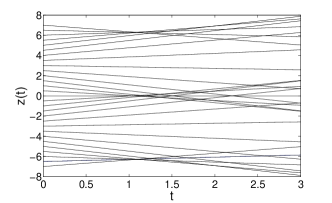
Figure 1: Paths $z(t)$ followed within the geometrical optics approximation by atoms expanding from a condensate with an initial phase $\theta(z)=\theta_{0}\cos(z)$.

At caustics one can observe spectacular diffraction effects berry . On slight deviation $\delta\tilde{z}\sim\theta_{0}^{-2/3}$ from the point $\tilde{z}_{n}$ the density displays a sharp drop, followed by aperiodic oscillations. The detailed shape of these oscillations can be found by further studying the integral in Eq. (11). We shall not do this here, but rather remark on the picture between caustics, at a point $\tilde{z}$ well separated from all $\tilde{z}_{n}$. In this case only Eq (13) remains to be satisfied, and since it can have several solutions, several saddle points will contribute to the integral in Eq. (11). Each saddle point contributes a term of order $\theta_{0}^{-1/2}$ which cancels the prefactor of $\theta_{0}^{1/2}$. Interference between different contributions — that is, between different rays arriving at the point $\tilde{z}$ at time $\tilde{t}$ — results in a density pattern with variations of order unity and spacing between fringes of order $\Delta\tilde{z}\sim 1/\theta_{0}$.

Our discussion has been limited to caustics of the simplest kind, referred to as folds in Ref. berry . More singular caustics, known as cusps can also occur. These stem from rays emerging from the points $\zeta_{n}=2\pi n$ with $n=0\,,\pm 1\,,\ldots$ and are visible only at a patricular time instant, $\tilde{t}=1$. The point is that for $\zeta_{n}=2\pi n$ and $\tilde{t}=1$ not only the first two but also the third derivative, $\partial^{3}_{\zeta}\varphi(\zeta,\tilde{z},\tilde{t})=\sin\zeta_{n}$, vanishes. The integral in Eq. (11) is then controlled by the fourth derivative, $\partial^{4}_{\zeta}\varphi(\zeta,\tilde{z},\tilde{t})=1$, and is of order $\theta_{0}^{-1/4}$, which implies that the reduced density at the points $\tilde{z}_{n}=2\pi n$ is at this time $|\psi(\zeta,\tilde{t})|^{2}\sim\theta_{0}^{1/2}$. Studying the integral in Eq. (11) in more detail, for values of $\tilde{t}$ and $\tilde{z}$ near $\tilde{t}=1$ and $\tilde{z}=2\pi n$ one can identify lines in the $\tilde{z}$-$\tilde{t}$ plane on which $|\psi(\zeta,\tilde{t})|^{2}$ drops from its maximum value, of order $\theta_{0}^{1/2}$, to values of order $\theta_{0}^{1/3}$. These lines have cusps at the most singular points, located at $\tilde{z}=2\pi n$ and $\tilde{t}=1$.

We illustrate these ideas using a numerical evaluation of Eq. (11) to obtain the relative density $|\psi(z,t)|^{2}$. The results are shown for several values of $\tilde{t}$ at fixed $\theta_{0}$ in Fig. 2, and for several values of $\theta_{0}$ at fixed $\tilde{t}$ in Fig. 3. In the large $\theta_{0}$ limit, caustics are located at: $\tilde{z}=0$ for $\tilde{t}=1$ at; $\tilde{z}=\pm 0.685$ for $\tilde{t}=2$; and at $\tilde{z}=\pm 1.598$ for $\tilde{t}=3$. The two figures show that $|\psi(z,t)|^{2}$ has peaks near these points, which grow in amplitude and become increasingly well defined with larger $\theta_{0}$.

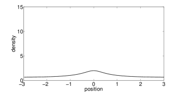
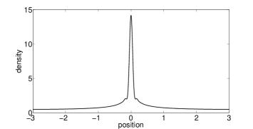
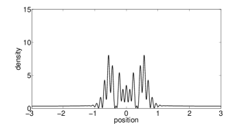
Figure 2: Relative density $|\psi(\tilde{z},\tilde{t})|^{2}$ as a function of position $\tilde{z}$, for $\theta_{0}=30$ and $\tilde{t}=0.5$ (top), $1$ (middle), and $2$ (bottom).

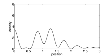
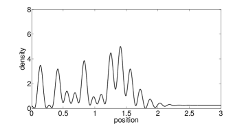
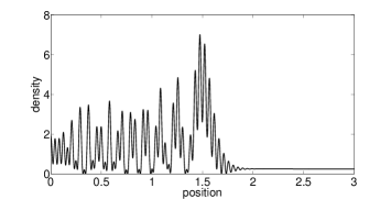
Figure 3: Relative density $|\psi(\tilde{z},\tilde{t})|^{2}$ as a function of position $\tilde{z}$, for $\tilde{t}=3$ and $\theta_{0}=10$ (top), $30$ (middle), and $100$ (bottom).

We now turn to a disordered potential $V(z)$, which we take to be Gaussian distributed with zero mean, amplitude $V_{0}$, correlation length $R_{0}$, and correlation function

$$\overline{V(z)V(z^{\prime})}=V_{0}^{2}f\left(\frac{z-z^{\prime}}{R_{0}}\right)\;.$$ (15)

Here and elsewhere, we use an overbar $\overline{\phantom{(}\dots\phantom{)}}$ to denote a disorder average. The function $f(\tilde{z})$ has unit amplitude and unit range, so that $f(0)=1$ and $f(\tilde{z})\to 0$ for $\tilde{z}\gg 1$. This implies for the impressed phase that its mean is zero and

$$\overline{\theta(z)\theta(z^{\prime})}=\theta_{0}^{2}f\left(\frac{z-z^{\prime}}{R_{0}}\right)$$ (16)

with $\theta_{0}=\pi V_{0}/2\hbar\omega_{\perp}$. The experimentally realised disordered potentials for cold atoms are optical speckle potentials (see Ref. kuhn for an extensive discussion) whose correlation function is

$$f(\tilde{z})=\frac{\sin^{2}(\tilde{z})}{\tilde{z}^{2}}\;.$$ (17)

Eq. (10) for $\psi(z,t)$ applies also for a disordered potential and the mechanism for caustic formation is qualitatively the same as for the harmonic potential discussed above. Caustics are due to rays emerging from singular points $z^{\prime}_{n}$ on which there are zeros of two or more derivatives with respect to $z^{\prime}$ of the overall phase in Eq. (10),

$$\frac{m}{2\hbar t}(z-z^{\prime})^{2}+\theta(z^{\prime})\;.$$

Since the impressed phase $\theta(z^{\prime})$ is now a random function, the formation of caustics of different types (fold, cusp or more singular) is a matter of probability. The typical time for caustic formation is $t^{*}=mR_{0}^{2}/\hbar\theta_{0}$. Using the relations $\frac{1}{2}m\omega_{\perp}^{2}a_{\perp}^{2}=\mu$ and $\theta_{0}=\pi V_{0}/2\hbar\omega_{\perp}$, the formation time can be written in terms of the experimentally controlled parameters as

$$t^{*}=\frac{4}{\pi\omega_{\perp}}\frac{\mu}{V_{0}}\left(\frac{R_{0}}{a_{\perp}}\right)^{2}\;.$$

It is quite straightforward to modify the theory of optical caustics berry ; hannay to the case of caustics in an expanding BEC, but we do not pursue this further here.

So far our discussion of caustics for the random case was qualitative and pertained to a specific, typical realisation of the disordered potential. We next present some quantitative analytic results for the second moment of the reduced density fluctuations,

$$\overline{|\psi(z,t)|^{4}}\equiv S(t)+1\;.$$

The averaging restores translational invariance and so eliminates the $z$-dependence. We denote the resulting (time-dependent) quantity by $S(t)+1$ in order to emphasise the analogy with speckle patterns in optics. There $S$ is called the scintillation index and it is a measure of spatial intensity fluctuations in the speckle pattern. For a uniform intensity $S$ is clearly zero, and for the standard speckle pattern, created by great number of interfering waves with random phases, in which the intensity has a Rayleigh distribution, $S$ is unity goodman . For the random screen problem, $S$ was studied as a function of distance $D$ from the screen in Ref. jakeman . It was shown there that, at first, $S$ increases with $D$ and reaches a maximum value larger that $1$ but then, with further increase in $D$, the value of $S$ drops and approaches $1$ for large $D$. We briefly outline a similar calculation for our problem.

Starting from Eq. (10) we write $|\psi(z,t)|^{4}$ as the product of four intergals. Performing the standard Gaussian average of the expression $\exp[{\rm i}(\theta(z_{1})-\theta(z_{2})+\theta(z_{3})-\theta(z_{4}))]$ then yields

$$S(t)+1=\frac{\theta_{0}}{2\pi\tilde{t}}\int\int{\rm d}\tilde{x}{\rm d}\tilde{y}\,{\rm e}^{-{\rm i}\theta_{0}\tilde{x}\tilde{y}/\tilde{t}}\,{\rm e}^{-\theta_{0}^{2}K(\tilde{x},\tilde{y})}\;.$$ (18)

The function $K(\tilde{x},\tilde{y})$ is defined by

$$K(\tilde{x},\tilde{y})=2-2f(\tilde{x})-2f(\tilde{y})+f(\tilde{x}+\tilde{y})+f(\tilde{x}-\tilde{y})\;,$$ (19)

where $f(\tilde{x})$ is the correlation function introduced in Eq. (15).

For $\theta_{0}\ll 1$, $\exp(-\theta_{0}^{2}K(\tilde{x},\tilde{y}))$ may be expanded as $1--\theta_{0}^{2}K(\tilde{x},\tilde{y})$. Then $S(t)$ is small, given by

$$S(t)=2\theta_{0}^{2}\left[1-\frac{1}{\sqrt{2\pi}}\int{\rm d}s\,(\sin s^{2}+\cos s^{2})f(s\sqrt{4\tilde{t}/\theta_{0}})\right]\;,$$ (20)

and saturates at the value $2\theta_{0}^{2}$ for $\tilde{t}\gg\theta_{0}$. This small $\theta_{0}$ regime was studied in Ref. clement . We turn to the more interesting case, $\theta_{0}\gg 1$, when caustics and related large interference effects can be observed. For this case no expansion in $\theta_{0}$ is possible and the analytical treatment becomes tedious jakeman . It is possible, however, to identify three distinct contributions to the integral in Eq. (18), each of which dominates at the appropriate time, and thus to derive an approximate expression:

$$S(t)+1 \approx \frac{2}{\pi}\int_{0}^{\infty}\frac{{\rm d}s}{s}\sin(\theta_{0}s/\tilde{t})\,{\rm e}^{-\frac{1}{2}\gamma\theta_{0}^{2}s^{2}}$$ (21)

$$-\frac{2}{\pi}\gamma\int_{0}^{\infty}{\rm d}s\,s\sin(s/\tilde{t})\ln(s/\theta_{0})\,{\rm e}^{-\frac{1}{2}\gamma s^{2}}$$

$$+2\left[1-{\rm erf}\left(\frac{1}{2\sqrt{\beta}\tilde{t}}\right)\right]\;,$$

where $\beta=|\partial^{2}_{\tilde{x}}f(\tilde{x})|_{\tilde{x}{=}0}|$ and $\gamma=|\partial^{4}_{\tilde{x}}f(\tilde{x})|_{\tilde{x}{=}0}|$. For the speckle pattern these numbers are $\beta=1/3$ and $\gamma=2/45$. The three terms in Eq. (21) make the dominant contribution to the scintillation index at different times. For short times, $\tilde{t}\ll 1$, the first term dominates and approaches $1$ as $\tilde{t}\to 0$, so that $S(t)$ drops to zero. The last term dominates in the opposite limit, $\tilde{t}\gg 1$. It approaches $2$, thus yielding the expected saturation value $S(t)=1$. The most interesting term, however, is the second one. It dominates for intermediate times, when $\tilde{t}\sim 1$, and it is proportional to $\ln\theta_{0}$, signalling the appearance at this time of caustics and the associated large density fluctuations.

Let us emphasize that the two basic requirements for our treatment are $\hbar\omega_{\perp}\ll\mu$ and $R_{0}\gg a_{\perp}$. The first inequality ensures that the size and energy of the condensate, while in equilibrium in the trap, is dominated by the interactions i.e. by the nonlinear term in the Gross-Pitaevskii equation. The second inequality is required for the validity of the two-stage-expansion scenario as well as of the ray picture on which the physics of caustics rests. To this point our treatment of density modulations in a BEC after expansion has been restricted to systems in which the relative amplitude of initial density fluctuations is small, which is the case when these are produced by a potential with amplitude $V_{0}\ll\mu$. It is in fact straightforward to generalise the discussion, to allow for an arbitrary value of $V_{0}$. A potential with amplitude $V_{0}\gtrsim\mu$ automatically implies impressed phase fluctuations with amplitude $\theta_{0}\gg 1$. That in turn justifies a stationary phase treatment of caustic formation, and according to this treatment, the atoms that form caustics come from short segments of the condensate, which have width proportional to $\theta_{0}^{-1/3}$ before the second stage of the expansion. Moreover, the density in these segments remains approximately constant during the first stage of expansion, provided $R_{0}\gg a_{\perp}$. To obtain the final relative density after expansion under these conditions, the value of $|\psi(z,t)|^{2}$ calculated from Eq. (10) should simply be multiplied by the initial relative density $|\psi(z^{\prime},0)|^{2}$ at a point $z^{\prime}$ determined from

$$z^{\prime}=z-\frac{\hbar t}{m}\partial_{z^{\prime}}\theta(z^{\prime})\;.$$ (22)

The consequences of this are most significant for $V_{0}\gtrsim\mu$, when the condensate before expansion is fragmented, having initial relative density $|\psi(z^{\prime},0)|^{2}=0$ for some values of $z^{\prime}$. In particular, it turns out that caustics are completely suppressed for $V_{0}\gg\mu$, because in this limit the initial density is zero at all points $z^{\prime}$ for which there is focussing of the emerging rays. To show this, note that focussing at time $t$ of atoms from $z^{\prime}$ occurs if

$$\partial^{2}_{z^{\prime}}\theta(z^{\prime})=-\frac{m}{\hbar t}\;,$$ (23)

that is to say, $\partial^{2}_{z^{\prime}}\theta(z^{\prime})$ must be negative. On the other hand, for $V_{0}\gg\mu$, the condensate before expansion occupies the neighbourhood of minima of the potential $V(x)$. In these regions $\partial^{2}_{z^{\prime}}V(z^{\prime})$ and hence $\partial^{2}_{z^{\prime}}\theta(z^{\prime})$ are positive, while at the points where $\partial^{2}_{z^{\prime}}\theta(z^{\prime})$ is negative, the initial density is zero. These ideas are illustrated schematically in Fig. 4.

Figure 4: Schematic illustration of the effect of condensate fragmentation before expansion on caustic formation after expansion. Middle panel: potential $V(z)$ and chemical potential $\mu$ before expansion. Lower panel: condensate density $|\psi|^{2}$ before expansion. Upper panel: position $z(t)$ reached by atoms after expansion as a function of starting point $z$, for three different expansion times, $t=0,t_{1}$ and $t_{2}$, with $0<t_{1}<t_{2}$. Caustics appear at turning points of $z(t)$ vs $z$, marked here for $t_{2}$ at $z_{a}$ and $z_{b}$. For the value of $\mu$ illustrated, the initial density is zero at points from which caustics would otherwise develop.

We next comment on a recent experiment chen which appears to satisfy the conditions for caustic formation. In this experiment $\mu/\hbar\omega_{\perp}=5.6$, $R_{0}=15\mu{\rm m}$, $a_{\perp}\lesssim 10\mu{\rm m}$ and the largest density variations were observed for $V_{0}=0.5\mu$, in a time of flight image at $t_{\rm ToF}=8{\rm ms}$, which is significantly larger than $1/\omega_{\perp}$. This value for $V_{0}$ corresponds to a phase amplitude $\theta_{0}=4.4$ which gives the caustic formation time $t^{*}=5{\rm ms}$. This is smaller than but comparable to the value of $t_{\rm ToF}$, and so the large density variations in Fig. 4(h) of Ref. chen can most likely be attributed to caustics. While the value $\theta_{0}=4.4$ does not lie deep within the large $\theta_{0}$ regime, the experiment was not designed for caustic observation. The results presented above should facilitate the optimisation of such experiments. We note further that at $V_{0}=\mu$, the largest potential amplitude for which results are reported in Ref. chen , the condensate before expansion appears to be fragmented (Fig. 4(i) of chen ) while there are no large density fluctuations after expansion (Fig. 4(j) of chen ). Both features are consistent with the scenario presented in our discussion of Fig. 4.

A related experiment has been described in Ref. clement together with a theoretical discussion appropriate for small $\theta_{0}$. Some of the parameters for this experiment take similar values to those of Ref. chen : $\mu/\hbar\omega_{\perp}=6.8$ and $V_{0}=0.41\mu$, giving $\theta_{0}=4.3$. However, the length scales $R_{0}=1.7\mu{\rm m}$ and $a_{\perp}=1.5\mu{\rm m}$ are about an order of magnitude smaller than the corresponding ones in chen . These lengths are also much smaller than the reported resolution ($8.5\mu{\rm m}$) of the imaging system and of the density fluctuations after expansion that are illustrated in Fig. 1 of Ref. clement . We note in addition that the time of flight used in clement (in the range $5$-$17{\rm ms}$) is about an order of magnitude larger than the value $t^{*}=1{\rm ms}$ we calculate from experimental parameters. Therefore caustics in this experiment should form and decay before time of flight images are made, and should have a smaller spacing than the resolution of the imaging system. For these reasons we do not expect the theory we have presented to apply directly to the measurements of Ref. clement .

III Strictly one dimension: many body correlations

In this section we discuss the possibility of caustic formation, in a system of interacting bosons, beyond the mean field approach. We assume here that $\hbar\omega_{\perp}$ is much larger than the characteristic interaction energy so that, with respect to transverse motion, all $N$ atoms in the trap reside in the ground state $\chi_{0}(\rho)$ of the harmonic oscillator, forming a strictly one-dimensional system. There is no confining potential in the axial direction, in which particles move on an interval $L$ with periodic boundary conditions. The axial motion is controlled by an effective one-dimensional Hamiltonian – the Lieb-Liniger model lieb ; olshanii . The chemical potential of the system, in equilibrium in the trap, differs from $\hbar\omega_{\perp}$ only by a small, interaction induced correction. This correction is crucial for the ground state properties of the gas. However, when the gas is released from the trap, the radial expansion will be governed not by the interaction, as happened for the many channel case ($\mu\gg\hbar\omega_{\perp}$) considered in Sec. II, but by the zero-point energy associated with radial motion. Thus, for a strictly one-dimensional system it is not possible to generate a large phase imprint from small initial density modulation during the radial expansion. Therefore, in this section as a means of impressing a phase we employ the second possibility, namely a short potential pulse, as mentioned in Sec. I. Phase imprinting of this kind has been proposed dobrek and used extensively to generate vortices in two and three dimensional condensates. The mechanism works as follows: starting at time $-\tau$ we apply to the system, in its ground state, a short potential pulse, of duration $\tau$ and of a prescribed spatial profile

$$V(z,t)=-\frac{\hbar}{\tau}\theta(z)\;,\qquad-\tau<t<0$$ (24)

where $\theta$ can be a deterministic or a random function of $z$. If the time interval $\tau$ is shorter than the characteristic times of the system, then at the time instant $t=0$ the axial part of the many-body wavefunction will acquire a phase

$$\Psi(z_{1},\ldots z_{N};t{=}0)=\exp\left[{\rm i}\sum_{j=1}^{N}\theta(z_{j})\right]\Phi_{0}(z_{1},\ldots z_{N})$$ (25)

where $\Phi_{0}(z_{1},\ldots z_{N})$ is the ground state wavefunction, prior to the action of the pulse, and is normalised to unity. (The complete wavefunction for the system in three dimensions of course also includes the radial factor $\prod_{j=1}^{N}\chi_{0}(\rho_{j})$.) At time $t=0$, just after this phase has been impressed, the trapping potential is switched off and the gas undergoes radial expansion. The initial Gaussian function, $\chi_{0}(\rho)$, will spread with time, retaining its Gaussian shape, and the density of the gas will evolve accordingly. Therefore we shall neglect interactions during the expansion, so that the gas is assumed to undergo free evolution and the $z$-dependent part of the many-body wavefunction evolves according to

$${\rm i}\hbar\frac{\partial\Psi(z_{1},\ldots z_{N};t)}{\partial t}=\left[\sum_{j=1}^{N}\left(-\frac{\hbar^{2}}{2m}\frac{\partial^{2}}{\partial z_{j}^{2}}\right)\right]\Psi(z_{1},\ldots z_{N};t)\;,$$ (26)

which is to be solved with the initial condition given in Eq. (25). This initial function contains all the information on the interacting groundstate, prior to the expansion.

We are interested in the one-dimensional, $z$-dependent part of the particle density

$$n_{1}(z,t)=N\int_{0}^{L}\left|\Psi(z,z_{2}\ldots z_{N};t)\right|^{2}{\rm d}z_{2}\ldots{\rm d}z_{N}\equiv\frac{N}{L}F(z,t)\;.$$ (27)

The actual, three-dimensional density $n(\rho,z,t)$ is obtained by multiplying $n_{1}(z,t)$ by the radial factor $|\chi(\rho,t)|^{2}$ – the spreading Gaussian. Initially, $F(z,t{=}0)=1$ but, as the expansion proceeds, $F(z,t)$ develops modulations in $z$, due to the initially impressed phase. In second quantised form

$$F(z,t)=\frac{L}{N}\langle\Psi|\hat{\psi}^{\dagger}(z,t)\hat{\psi}(z,t)|\Psi\rangle$$ (28)

where $|\Psi\rangle$ is the initial state vector, defined in position representation in Eq. (25), while $\hat{\psi}^{\dagger}(z,t)$ and ${\psi(z,t)}$ are the free field operators

$$\hat{\psi}^{\dagger}(z,t)=\frac{1}{\sqrt{L}}\sum_{k}{\rm e}^{{\rm i}\frac{\hbar k^{2}}{2m}t-{\rm i}kz}a_{k}^{\dagger}\;$$ (29)

with creation and annihilation operators $a^{\dagger}_{k}$ and $a^{\phantom{\dagger}}_{k}$ that satisfy the commutation relation $[a^{\phantom{\dagger}}_{q},a^{\dagger}_{k}]=\delta_{k,q}$.

Using Eq. (29) and the relation

$$\langle\Psi|\hat{\psi}^{\dagger}(x)\hat{\psi}(y)|\Psi\rangle={\rm e}^{{\rm i}(\theta(y)-\theta(x))}\langle\Phi_{0}|\hat{\psi}^{\dagger}(x)\hat{\psi}(y)|\Phi_{0}\rangle\;,$$ (30)

Eq. (28) can be written as

$$F(z,t)=\int\frac{{\rm d}p}{2\pi}|G_{p}(z,t)|^{2}n(p)\;,$$ (31)

where $n(p)$ is the momentum distribution function

$$n(p)=\frac{L}{N}\int{\rm d}z\langle\hat{\psi}^{\dagger}(z)\hat{\psi}^{\phantom{\dagger}}(0)\rangle{\rm e}^{-{\rm i}pz}$$ (32)

normalised so that

$$\int\frac{{\rm d}p}{2\pi}n(p)=1\;.$$ (33)

The function $G_{p}(z,t)$ is

$$G_{p}(z,t)=\sqrt{\frac{m}{2\pi{\rm i}\hbar t}}\int{\rm d}\zeta\exp\left[\frac{{\rm i}m}{2\hbar t}(z-\zeta)^{2}+{\rm i}\theta(\zeta)-{\rm i}{p}\zeta\right]\;.$$ (34)

In the mean field approach $n(p)=2\pi\delta(p)$ and the expression for $G_{p}(z,t)$ reduces to that for $\psi(z,t)$ given in Eq. (10) of Sec. II. Such behaviour corresponds to the non-interacting limit of the Leib-Liniger gas which, under radial expansion, will exhibit large density variations and caustics, as discussed in Sec. II. Below we show that interactions inhibit caustic formation, and derive a condition for caustics to survive in the presence of interactions.

The treatment of the integral in Eq. (34) is along the same lines as in Sec II. Caustics originate from rays emerging from points $\zeta_{n}$ at which the second derivative of the phase in Eq. (34) vanishes. Since this derivative does not contain $p$, we have the familiar condition for the singular points, $\partial^{2}_{\zeta}\theta(\zeta)=-m/\hbar t$ at $\zeta=\zeta_{n}$. The first derivative, however, now contains $p$ so that the analogue of Eq. (13), for an arbitrary function $\theta(\zeta)$ and keeping all physical dimensions, is

$$z=\zeta+\frac{\hbar t}{m}\left(\partial_{\zeta}\theta(\zeta)-p\right)\;.$$ (35)

This is essentially the definition of a ray, emerging from a point $\zeta$, and having a particular value of $p$. The dependence on $p$ implies that the rays emerging from the same singular point $\zeta_{n}$, but having different values of $p$, will not arrive at the point $z$ at the same time. Thus focussing, which is the essence of the phenomenon of caustics, will be suppressed and caustics will get washed out. The condition for the existence of caustics follows from the integral in Eq. (34). Assuming that the function $\theta(\zeta)$ has a characteristic amplitude $\theta_{0}$ and scale of variation $R_{0}$, and expanding the phase in Eq. (34) near a singular point $\zeta_{n}$, one obtains a contribution $C\theta_{0}R_{0}^{-3}\eta^{3}-{p}\eta$ where $\eta=\zeta-\zeta_{n}$ and $C$ is a constant of order $1$. Caustics originate from the $\eta^{3}$-term and the relevant range of integration is $\eta\lesssim R_{0}\theta_{0}^{-1/3}$. Therefore, if the contributing values of $p$, defined by the range over which $n(p)$ is significant, are such that $R_{0}p\theta_{0}^{-1/3}\ll 1$, then caustics will survive. Since most of the weight of the momentum distribution $n(p)$ is concentrated in the interval $p\lesssim 1/\xi$ haldane ; astrakharchik , where $\xi$ is the coherence length for the Bose gas, we arrive at the condition $\theta_{0}^{1/3}\xi/R_{0}\gg 1$. It should be supplemented by the requirement that, for a caustic to be formed and visible, there must be many particles in the region from which it originates. This condition is $n_{1}R_{0}\theta_{0}^{-1/3}\gg 1$. Both conditions can be easily satisfied in the weak interaction limit where $\xi n_{1}\gg 1$. The situation is different in the opposite case of strong interactions, or hard-core bosons. In this case $\xi\approx 1/n_{1}$, and so caustics are absent in the strongly interacting limit.

IV Two dimensional systems

In this section we consider expansion of a quasi-two dimensional condensate after release from a trap with strong axial and weak radial confinement, characterised as in Sec II by frequencies $\omega_{z}$ and $\omega_{\perp}$ but here with $\omega_{z}\gg\omega_{\perp}$. Again we neglect the weaker confinement, restricting our discussion to times $t\ll 1/\omega_{\perp}$ after release of the trap, and treat a BEC with initial density modulations, which are converted during expansion into an impressed phase. A difference between the two-dimensional and one-dimensional geometries is that caustics in two dimensions consist of lines rather than points. Another difference is that, within the Thomas-Fermi approximation, a two-dimensional condensate in a disordered potential undergoes a percolation transition at a finite critical value of disorder strength. Because caustic formation is essentially a local pheomenon, the network of caustic lines does not show any critical behaviour that reflects this percolation transition, although it does change with disorder strength.

The distinction between the initial and late phases of expansion is not as sharp in two-dimensions as it is in one dimension. The reason for this is that the characteristic density near the center of the trap decreases with time $t$ as $t^{-1}$ in two dimensions and as $t^{-2}$ in one dimension, with the result that the impressed phase grows logarithmically at long times in two dimensions, but reaches a limiting value in one dimension. We neglect this logarithmic growth and take the impressed phase to have a definite value

$$\theta({\bf r}_{\perp})\sim\frac{V({\bf r}_{\perp})}{\hbar\omega_{z}}\;$$ (36)

at times large compared to $1/\omega_{z}$, with characteristic amplitude $\theta_{0}$ and length scale $1/k_{0}$. In this approximation the wavefunction during the second phase of expansion can be factorised as

$$\Psi({\bf r}_{\perp},z,t)=\Phi({\bf r}_{\perp},t)\psi(z,t)\;.$$ (37)

For a two-dimensional system the axial part is given by a scaling function pitaevskii and our interest is in the evolution of the planar part, $\Phi({\bf r}_{\perp},t)$. In analogy with Eq. (10), it is given at late times by

$$\Phi({\bf r}_{\perp},t)=\frac{m}{2\pi{\rm i}\hbar t}\int{\rm d}^{2}{\bf r}_{\perp}^{\prime}\exp\left[\frac{{\rm i}m}{2\hbar t}|{\bf r}_{\perp}-{\bf r}_{\perp}^{\prime}|^{2}+{\rm i}\theta({\bf r}_{\perp}^{\prime})\right]\;.$$ (38)

As in quasi-one dimensional systems, caustics are formed for $\theta_{0}\gg 1$ at values of the scaled time $\tilde{t}\gtrsim 1$, and in this regime Eq. (38) can be evaluated using the stationary phase method. The saddle points in ${\bf r}_{\perp}^{\prime}$ are the solutions to

$$\frac{m}{\hbar t}({\bf r}_{\perp}^{\prime}-{\bf r}_{\perp})+{\bf\nabla}_{{\bf r}_{\perp}^{\prime}}\theta({\bf r}_{\perp}^{\prime})=0\;.$$ (39)

In the leading approximation, one such saddle point, at ${\bf r}_{\perp}^{\prime}={\bf r}_{\perp}^{*}$, makes a contribution to $\Phi({\bf r}_{\perp},t)$ of modulus $[{\rm det}M({\bf r}_{\perp}^{*})]^{-1/2}$, where

$$M({\bf r}_{\perp}^{\prime})=\left(\begin{array}[]{cc}\frac{m}{\hbar t}+\partial^{2}_{x^{\prime}}\theta({\bf r}_{\perp}^{\prime})&\partial_{x^{\prime}}\partial_{y^{\prime}}\theta({\bf r}_{\perp}^{\prime})\\ &\\ \partial_{y^{\prime}}\partial_{x^{\prime}}\theta({\bf r}_{\perp}^{\prime})&\frac{m}{\hbar t}+\partial^{2}_{y^{\prime}}\theta({\bf r}_{\perp}^{\prime})\end{array}\right)\;.$$ (40)

Caustics stem from those saddle points at which ${\rm det}M({\bf r}_{\perp}^{*})=0$. Atoms in the expanding condensate originating from these points are focussed in such a way that the density $|\Phi({\bf r}_{\perp},t)|^{2}$ is divergent within this approximation, which is equivalent to geometrical optics. To find the density in the vicinity of caustics, it would be necessary to take into account higher derivatives of $\theta({\bf r}_{\perp})$ when calculating the integral in Eq. (38). We do not do this, restricting ourselves instead to a discussion of the positions of caustics. The condition ${\rm det}M({\bf r}_{\perp}^{*})=0$ defines a set of lines in the atomic cloud after the initial phase of expansion, which give rise to caustics. Both the number and the shape of these lines in the initial plane depend on the time at which density in the expanding cloud is to be measured, but they have fixed limits for $\tilde{t}\gg 1$. Atoms starting from points on these lines travel with velocity $(\hbar/m)\nabla\theta$, and reach points in the cloud at time $t$ with coordinates ${\bf r}_{\perp}$ given by the solutions to Eq. (39). In this way lines in the initial plane are mapped to moving lines of high density in the expanding cloud.

To illustrate these general ideas, consider the example of a periodic impressed phase

$$\theta({\bf r}_{\perp})=\theta_{0}(\cos k_{0}x+\cos k_{0}y)\;.$$ (41)

In this case the condition ${\rm det}M({\bf r}_{\perp}^{*})=0$ yields

$$(\tilde{t}^{-1}-\cos k_{0}x^{*})(\tilde{t}^{-1}-\cos k_{0}y^{*})=0\;,$$ (42)

defining two sets of parallel lines in the initial plane, $x^{*}=k_{0}^{-1}\cos^{-1}(1/\tilde{t})$ and $y^{*}=k_{0}^{-1}\cos^{-1}(1/\tilde{t})$. Caustics derive from these, forming two similar sets of lines in the final plane, $x=x^{*}-\tilde{t}\sin k_{0}x^{*}$ and $y=y^{*}-\tilde{t}\sin k_{0}y^{*}$ respectively.

The consequences in two dimensions of a potential $V({\bf r}_{\perp})$ strong enough to generate significant density modulations before expansion can be discussed for large $\theta_{0}$ using the same approach as in Sec. II. In this way we find that two conditions must be satisfied in order that a line segment in the initial plane will give rise to a caustic after expansion: it is necessary, first, that ${\rm det}M({\bf r}_{\perp})=0$ and, second, that the initial relative density $|\Phi({\bf r}_{\perp},0)|^{2}$ is non-zero on the line. In consequence, as the potential strength is increased, or the chemical potential is reduced, caustic lines first develop breaks, and then disappear altogether. Such an evolution with decreasing $\mu$ of the lines in the inital plane that generate caustics is illustrated in Fig 5 for the periodic potential that underlies Eq. (41).

Figure 5: Effect of decreasing $\mu$ in the condensate before expansion, on caustic formation in two dimensions, illustrated for a periodic potential $V({\bf r}_{\perp})$. Each of the four panels shows the initial plane. Caustics evolve from lines with ${\rm det}M({\bf r}_{\perp})=0$ and $|\Phi({\bf r}_{\perp},0)|^{2}>0$. These are marked in bold, while lines with ${\rm det}M({\bf r}_{\perp})=0$ and $|\Phi({\bf r}_{\perp},0)|^{2}=0$ are shown dotted. Panel (a): large $\mu$, $|\Phi({\bf r}_{\perp},0)|^{2}>0$ everywhere; (b) on reducing $\mu$, the condensate develops small holes but percolates, while caustics become fragmented; (c) reducing $\mu$ further, the condensate reaches the percolation threshold, but caustics show no signature of this; (d) reducing $\mu$ still further, caustics shrink and eventually disappear.

The theory of caustic formation resulting from a random phase $\theta({\bf r}_{\perp})$ is analogous to the treatment of the phase screen problem, which has been studied extensively for two-dimensional systems in the context of optics berry . In particular, the morphology of caustic lines for the random case is discussed in berry2 .

V Fermions

It is interesting to ask about problems similar to the ones we have discussed, but with fermions in place of bosons. To be specific, consider expansion of a strictly one dimensional system with an imprinted phase, as in Sec. III, but for non-interacting fermions rather than interacting bosons. Restricting our attention to the expectation value of the density as a function of position and time, the effects of particle statistics enter the main result, Eq. (31), only through the momentum distribution of particles before expansion. The criterion for formation of caustics in the expanding Fermi gas is therefore the same as for the Lieb-Liniger gas, but with the Fermi wavelength $\lambda_{\rm F}$ taking the place of the coherence length $\xi$ in the expressions given in Sec. III. Hence caustics are absent from the Fermi gas, for the same reason as in the Bose gas with hard-core interactions. There are nevertheless differences between non-interacting fermions and hard-core bosons. They stem from the Fermi surface discontinuity in the momentum distribution. Within the approximations of geometrical optics, this discontinuity leads to sharp peaks in the derivative of the relative density $F(z,t)$ with respect to position $z$ or time $t$. To show this, we note from Eq. (34) that

$$\partial_{z}|G_{p}(z,t)|^{2}=\frac{m}{\hbar t}\partial_{p}|G_{p}(z,t)|^{2}\;.$$ (43)

With Eq. (31) this yields

$$\partial_{z}F(z,t) = -\frac{m}{\hbar t}\int\frac{{\rm d}p}{2\pi}|G_{p}(z,t)|^{2}\partial_{p}n(p)$$ (44)

$$= \frac{m}{2\hbar p_{\rm F}t}\left[|G_{p_{\rm F}}(z,t)|^{2}-|G_{-p_{\rm F}}(z,t)|^{2}\right]\,,$$

where $p_{\rm F}$ is the Fermi wavevector. The behaviour of $G_{p}(z,t)$ has been analysed in Sec. II: the value of $p$ influences the position of caustics but not their formation. The Fermi gas therefore shows the same extrema in the derivative of the density as are found for a BEC in the density itself.

VI Summary

We have discussed free motion of one and two dimensional atomic gases with an initial impressed phase that varies periodically or randomly as a function of position. Gradients of this phase represent initial velocities and lead to density variations that grow with time. The characteristic amplitude $\theta_{0}$ and size $R_{0}$ of spatial variations of this phase are key parameters. The limit $\theta_{0}\gg 1$ is both the most interesting regime, because density maxima are largest, and a tractable one theoretically, because a treatment analogous to geometrical optics provides the leading approximation. The evolution of atomic density fluctuations with time has close links to problems in optics involving caustic formation. In the context of atomic gases, caustics are maxima of density, near points in one dimensional systems or along lines in the two dimensional case. For atoms of mass $m$ they form at a characteristic time $t^{*}=mR_{0}^{2}/\hbar\theta_{0}$ and at longer times $t$ the density within a caustic decays as $t^{-1}$. Since caustics originate from small regions of the initial atomic cloud, variations in the initial density simply modulate the density on caustics. In particular, caustic formation is suppressed during expansion of a fragmented condensate if the initial density is zero at points that would otherwise be the origin for caustics.

We have argued that a recent experiment chen in which large density modulations are observed in an elongated BEC after release from a disordered potential should be understood in terms of caustic formation. For the future it would be of interest to design experiments with larger values of $\theta_{0}$ for both one and two dimensional systems.

- (1) See: L. D. Landau and E. M. Lifshitz, The classical theory of fields, 4th Ed., (Elsevier, Oxford, 1975).
- (2) M. V. Berry, J. Phys. A 10, 2061 (1977); Adv. Phys. 25, 1 (1976).
- (3) S. Dettmer, D. Hellweg, P. Ryytty, J. J. Arlt, W. Etmer, K. Stengstock, D. S. Petrov, G. V. Shlyapnikov, H. Kreutzmann, L. Santos, and M. Lewenstein, Phys. Rev. Lett. 87, 160406 (2001).
- (4) D. Clément, P. Bouyer, A. Aspect, and L. Sanchez-Palencia, Phys. Rev. A 77, 033631 (2008).
- (5) Y. P. Chen, J. Hitchcock, D. Dries, M. Junker, C. Welford, and R. G. Hulet, Phys. Rev. A 77, 033632(2008).
- (6) L. Pitaevskii and S. Stringari, Bose-Einstein Condensation (Oxford University Press, Oxford, 2004).
- (7) J. H. Hannay, J. Phys. A 16, L61 (1983).
- (8) R. C. Kuhn, O. Sigwarth, C. Miniatura, D. Delande, and C. A. Muller, New J. Phys. 9, 161 (2007).
- (9) J. W. Goodman, Statistical Optics (Wiley, New York, 1985).
- (10) E. Jakeman and J. G. McWhirter, J. Phys. A 10, 1599 (1977).
- (11) E. H. Lieb and W. Liniger, Phys. Rev. 130, 1605 (1963).
- (12) M. Olshanii, Phys. Rev. Lett. 81, 938 (1998).
- (13) L. Dobrek, M. Gajda, M. Lewenstein, K. Sengstock, G. Birkl, and W. Ertmer, Phys. Rev. A 60, R3381 (1999).
- (14) F. D. M. Haldane, Phys. Rev. Lett. 47, 1840 (1981).
- (15) G. E. Astrakharechik and S. Giorgini, J. Phys. B 39, S1 (2006).
- (16) M. V. Berry, Proc. Symp. App. Maths 36, 13 (1980).