Multi-wavelength Variability of the Broad Line Radio Galaxy 3C 120

Abstract

We present results from a multi-year monitoring campaign of the broad-line radio galaxy 3C 120, using the Rossi X-ray Timing Explorer (RXTE) for nearly five years of observations. Additionally, we present coincident optical monitoring using data from several ground-based observatories. Both the X-ray and optical emission are highly variable and appear to be strongly correlated, with the X-ray emission leading the optical by 28 days. The X-ray power density spectrum is best fit by a broken power law, with a low-frequency slope of $-1.2$, breaking to a high-frequency slope of $-2.1$, and a break frequency of $\log\nu_{\rm b}=-5.75$ Hz, or 6.5 days. This value agrees well with the value expected based on 3C 120’s mass and accretion rate. We find no evidence for a second break in the power spectrum. Combined with a moderately soft X-ray spectrum ($\Gamma=1.8$) and a moderately high accretion rate ($\dot{m}/\dot{m}_{\rm Edd}\sim 0.3$), this indicates that 3C 120 fits in well with the high/soft variability state found in most other AGNs. Previous studies have shown that the spectrum has a strong Fe K$\alpha$ line, which may be relativistically broadened. The presence of this line, combined with a power spectrum similar to that seen in Seyfert galaxies, suggests that the majority of the X-ray emission in this object arises in or near the disk, and not in the jet.

1 Introduction

Variability has long been recognized as a universal property of active galactic nuclei (AGN). Produced close to the nucleus, X-ray emission is often the most variable of any waveband. Early analysis of X-ray variability showed that the power density spectrum (PDS) follows a power law, or “red noise” form, $P\propto\nu^{\alpha}$, where $P$ is the variability power at frequency $\nu$, and $\alpha$ is the power law slope (McHardy & Czerny 1987; Lawrence & Papadakis 1993). No break frequency was seen, due to the short nature of the observations. Later results demonstrated that most AGN can be modeled by a broken power law PDS, where the slope changes from being relatively shallow at low frequencies to some steeper value above a critical break frequency (Edelson & Nandra 1999; Uttley et al. 2002; Markowitz et al. 2003).

This behavior closely mirrors what is seen in galactic black hole X-ray binaries (BHXRBs), which contain black holes with masses of only a few $\mbox{M}_{\odot}$. Much of the work connecting AGN and BHXRBs has focused on Cygnus X-1, which is one of the brightest and most well-studied BHXRBs. Cygnus X-1 is commonly in one of two different variability states: a low/hard state with a low flux level, hard X-ray spectrum, and a PDS with 2 separate breaks; and a high/soft state, with higher X-ray flux, soft (steep) X-ray spectrum, and a singly-broken PDS (Revnivtsev et al. 2000; McHardy et al. 2004). Based on scaling of the break frequencies with black hole mass and accretion rate, nearly all of the AGN studied to date match best with the high/soft state, showing only one break in their power spectrum (Akn 564 is the sole exception, see McHardy et al. 2007)

The break frequency scales over more than 6 orders of magnitude in mass, if one extrapolates the break frequencies of Cygnus X-1 (Markowitz et al. 2003). The variability state is thought to be driven by the accretion rate, with the high/soft state correlating to a higher accretion rate which may push in the inner edge of the accretion disk (Esin et al. 1997; Churazov et al. 2001). This has been combined into a ‘fundamental plane’ of variability by McHardy et al. (2006), with mass and bolometric luminosity uniquely determining the break timescale.

In Seyfert 1 galaxies, where no jet is detected, the X-ray emission is mainly thought to arise in or near the accretion disk (Haardt & Maraschi 1991, 1993). This variability may also be connected to the broad line region (BLR), as McHardy et al. (2006) showed that the break timescale is also related to the full-width half-maximum (FWHM) of H$\beta$ emission. Thus far, efforts to analyze the X-ray variability of AGN with jets have been limited. Furthermore, the connection between the X-ray variability and the jet in AGN needs to be defined better than has been possible thus far.

The nearby ($z=0.033$) broad-line radio galaxy (BLRG) 3C 120 is an interesting target for this type of variability analysis. Originally classified as a type 1 Seyfert, 3C 120 was first discovered as an X-ray source by Forman et al. (1978) using the Uhuru observatory. A superluminal radio jet was later discovered by Walker et al. (1982). 3C 120 has also exhibited extreme optical variability at times (Webb et al. 1988; French & Miller 1980), with variations of more than half a magnitude on timescales of a few days. Marscher et al. (2002) used coordinated VLBI and RXTE observations to show that dips in the X-ray flux corresponded with ejections of superluminal knots of bright emission along the jet.

The structure of our paper is as follows: in §2 we discuss our observations and data reduction methods, discuss the stationarity of the light curve in §3, present results for X-ray and optical correlation in §4, present results from Monte Carlo simulations of the power spectrum in §5, and in §6 we discuss implications of our results and present conclusions.

2 Observations and Data Reduction

We have observed 3C 120 for several years at both optical and X-ray wavelengths, on a variety of timescales. In Table 1 we summarize our monitoring at each timescale. Below we detail our data reduction methods.

2.1 X-ray Data

All of our X-ray observations come from a multi-year monitoring program using RXTE. 3C 120 was monitored three times per week from 2002 March until 2007 January, excluding several 8-week periods when the object’s proximity to the Sun prevented observations. We refer to these data as the ‘long term’ light curve.

Additionally, from 14 November 2006 until 12 January 2007 3C 120 was observed every 6 hours during this period. These data are referred to as the ‘intermediate’ sampling data. Finally, 3C 120 was monitored nearly continuously from 13–22 December 2002, which we refer to as the ‘short’ term light curve. The short term light curve was binned to an interval of 4000s, because AGN typically do not show variability on shorter timescales, and such binning also improves computational timescales greatly.

We use only data taken by PCU detectors 0 and 2, in STANDARD2 data mode. All of our data were reduced using FTOOLS v5.2 software, provided by HEASARC. Data were excluded if the Earth elevation angle was $<15^{\circ}$, pointing offset $>0.02^{\circ}$, time since South Atlantic Anomaly passage $<30$ minutes, or electron noise $>0.1$ units. Counts were extracted from the top PCU layer only to maximize the signal to noise ratio.

Figure 1 shows the light curves for all three timescales. In all subsequent analysis, we do not interpolate any gaps in the light curves with the exception of the short term light curve, which has a larger number of gaps due to Earth occultations and other observing programs, and a lower variance than the other data sets. The 2–10 keV X-ray spectral index remained relatively constant throughout our observations, with all ObsIDs showing an average $\Gamma_{\rm X}=1.8$ with a standard deviation of 0.1, where $\nu F_{\rm x}\propto\nu^{-\Gamma_{\rm X}}$.

2.2 Optical Data

We have also monitored 3C 120 at optical wavelengths during most of our long term X-ray observations using multiple ground-based observatories. From 2004 September until 2007 January, optical data were taken using the 2 m Liverpool Telescope at La Palma, Canary Islands, Spain. We also supplement these observations using data from the 1.8 m Perkins Reflector at Lowell Observatory in Arizona, and the 1.3 m SMARTS consortium telescope at Cerro Tololo Inter-American Observatory in Chile. Data were reduced using standard methods, and a correction applied, if necessary, to match the flux measured by the Liverpool Telescope.

All of our optical data were binned to the same 2.33 day timescale as our long term X-ray light curve, giving us a total of 124 data points. Figure 2 shows the binned optical light curve, along with the relevant portion of the X-ray light curve.

3 Stationarity

Before we can undertake any meaningful analysis of variability, we must first determine whether or not the data are stationary. In a statistical sense, stationarity means the underlying variability process does not change over time. We can test for this using the “$S$” statistic of Papadakis & Lawrence (1995), which measures stationarity in the power spectrum. The light curve is divided into two equal halves, the power spectrum is computed for each half, and then the two are compared using the $S$ statistic, where $S$ is defined as:

$$S(\nu)=\frac{\log P_{1}(\nu)-\log P_{2}(\nu)}{\sqrt{{\rm var}[\log P_{1}(\nu)]+{\rm var}[\log P_{2}(\nu)]}}$$

where $P_{\rm 1,2}(\nu)$ are the power spectra for each half of the light curve, and ${\rm var}[\log P_{\rm 1,2}]=0.31$ (Papadakis & Lawrence 1993). We can then sum over all frequencies to find the test statistic $S$,

$$S=\frac{1}{N}\sum_{n=1}^{n_{max}}S(\nu_{n})$$

where $N$ is the total number of frequencies for which we have calculated the power spectrum. For two identical power spectra, $S$ will have a Gaussian distribution with zero mean and unit variance. Or in other words, if $|S|<1$ we can reasonably assume the variability is stationary.

For our long-term light curve, we find that $S=0.238$. This indicates that the variability in 3C 120 is stationary, and that the fundamental variability mechanism does not change during the 4+ years of our observations.

4 X-ray/Optical Cross Correlation

To examine the relationship between the X-ray and optical emission, we use the cross correlation function (CCF). The traditional CCF requires evenly sampled data, and can be computationally intensive. Because of observing constraints, neither our X-ray nor optical data are evenly sampled. To solve this issue, we use the discrete correlation function (DCF) of Edelson & Krolik (1988), which allows for cross correlation of two unevenly sampled data sets.

The DCF is shown in Figure 3, with positive lag indicating X-ray emission leading the optical. Because the DCF has a broad shape, determining a precise maximum value may not be the best way to quantify any possible lag, so we fit the DCF with a Gaussian curve. The curve provides an excellent fit to the DCF, and has a maximum at a peak lag of +28 days, at a correlation coefficient of 0.8.

As discussed in Uttley et al. (2003), traditional error bars are inadequate for assessing the significance of the DCF, because adjacent data points in the light curve are “red noise” data and not uncorrelated. Therefore we use Monte Carlo simulations to assess the significance of the correlation. Our method is as follows.

We began by simulating 2 independent red noise light curves, using the method of Timmer & Koenig (1995). One light curve was given a power spectrum identical to the X-ray PDS in §5, and the other light curve was simulated using the measured optical PDS, which shows a slope of $-1.6$ with no measured break (Ryle et al. 2009, in preparation). The two light curves were then re-sampled in the same fashion as the original light curves, and random noise was added in the form of a Gaussian random with mean of zero and standard deviation equal to the average observed error. The light curves were then correlated, looking for any cases where the maximum correlation coefficient was greater than 0.8. Out of 1000 simulations, this was only the case 2 times. Therefore the correlation coefficient of $r=0.8$ seen in the data is significant at more than 99% confidence.

To explore the significance of the measured lag, we use the Flux Randomization / Random Subset Selection (FR/RSS) technique (White & Peterson 1994; Peterson et al. 1998). Briefly, random errors are added to each light curve, using the same method as above. For each light curve with $N$ data points total, the same number of data points are chosen at random from each curve, and duplicates are rejected. This typically results in a fraction of $\sim 1/e$ points rejected from each new light curve. The curves are then cross correlated as before, the DCF is fit with a Gaussian, and the centroid noted. This is done a large number of times (1000 simulations), and the distribution of DCF centroid values is used to estimate uncertainties.

As noted by Maoz & Netzer (1989), distributions of lags are nonnormal and the standard deviation is not a good estimate of the uncertainty in the lag. Therefore similar to Peterson et al. (1998), we quote uncertainties at $\pm\Delta\tau_{68}$, where 68.27% of the realizations yield results between $\tau_{\rm median}-\Delta\tau_{68}$ and $\tau_{\rm median}+\Delta\tau_{68}$, which corresponds to a $1\sigma$ error for a normal distribution. Using this method, we estimate the lag for 3C 120 as $28.73_{-5.87}^{+6.19}$ days. The distribution of lags measured using the FR/RSS method is shown in Figure 4.

5 X-ray Power Density Spectrum

The large amount of X-ray data, covering a wide variety of timescales, allow us to calculate the power density spectrum (PDS) over more than 4 decades of frequency. Calculating the PDS for any discretely sampled, finite length data set is inherently problematic, suffering from a number of complications such as windowing, aliasing, and red noise leakage. To avoid these complications, we follow the method of Uttley et al. (2002), which we outline briefly below.

We begin by calculating the square modulus of the discrete Fourier transform for each light curve, using the formula

$$|F(\nu)|^{2}=\left[\sum_{i=1}^{N}f(t_{i})\cos(2\pi\nu t_{i})\right]^{2}+\left[\sum_{i=1}^{N}f(t_{i})\sin(2\pi\nu t_{i})\right]^{2},$$

where $t_{i}$ are the light curve data points, and $|F(\nu)|^{2}$ is calculated at evenly spaced frequencies from $\nu_{\rm min}=1/T$ to $\nu_{\rm Nyq}=N/2T$, where $T$ is the total duration of the light curve. The PDS is then normalized using the fractional rms squared normalization (Miyamoto et al. 1991),

$$P(\nu)=\frac{2T}{\mu^{2}N^{2}}|F(\nu)|^{2},$$

where $\mu$ is the average count rate of the light curve. The observed PDS is then binned geometrically every factor of 1.5 (0.18 in the logarithm).

Monte Carlo simulations are then used to find the best-fit model for the observed PDS. A simulated light curve is generated based on an input model power spectrum, based on the method of Timmer & Koenig (1995). The simulated light curve is created with at least 100 times the duration of the actual light curve, to avoid the problem of variability power from longer timescales being shifted to shorter timescales (red noise leakage). The simulated light curve is then split into 100 segments of equal length.

Because our data are not continuously sampled, power above the Nyquist frequency can also be aliased back into the power spectrum. To avoid this, our simulated light curves have a time resolution of $0.1T_{\rm samp}$, where $T_{\rm samp}$ is the sampling timescale of the light curve.

The simulated light curves are then re-sampled in the same fashion as the observed light curves. The PDS is then calculated for each of the 100 curves, and binned by factors of 1.5. The 100 individual power spectra are then averaged, and error bars for each data point are calculated from the rms spread of the individual PDS points.

Poisson noise is added to the simulated power spectra using

$$P_{\rm Poisson}=\frac{\sum_{i=1}^{N}\sigma(i)^{2}}{N(\nu_{\rm Nyq}-\nu_{\rm min})},$$

where $\sigma(i)$ are the error bars for each point in the light curve. We can also estimate analytically the amount of power which will be aliased back into the PDS from frequencies above the minimum resolution of the simulations. This power is given by:

$$P_{\rm Alias}=\frac{1}{\nu_{\rm Nyq}-\nu_{\rm min}}\int_{\nu_{\rm Nyq}}^{1/(2T_{\rm exp})}P(\nu)d\nu,$$

where $T_{\rm exp}$ is the exposure time of our observations, typically $\sim 1$ ksec.

To determine the goodness of fit of the model, we use a modified $\chi^{2}$ fit. First we compare the observed PDS to average of the simulated power spectra:

$$\chi_{\rm obs}^{2}=\sum_{\nu}\frac{(\overline{P_{\rm sim}(\nu)}-P_{\rm obs}(\nu))^{2}}{(\Delta\overline{P_{\rm sim}(\nu)})^{2}},$$

where $P_{\rm obs}(\nu)$ is the observed PDS at frequency $\nu$, $\overline{P_{\rm sim}(\nu)}$ is the average of the simulated power spectra at that same frequency, and $\Delta\overline{P_{\rm sim}(\nu)}$ is the rms spread of the power spectra.

We then randomly choose 1000 combinations of simulated power spectra at each sampling rate. We then calculate $\chi_{\rm dist}^{2}$, where:

$$\chi_{\rm dist}^{2}=\sum_{\nu}\frac{(P_{\rm sim}(\nu)-\overline{P_{\rm sim}}(\nu))^{2}}{\Delta\overline{P_{\rm sim}}(\nu)^{2}}.$$

Of these 1000 combinations, the fraction where $\chi_{\rm obs}$ is smaller than $\chi_{\rm dist}$ represents the probability of acceptance of the model, i.e., the probability that the model provides an acceptable fit to the data. This process is repeated for a grid of slopes and break frequencies, to determine the parameters which yield the highest probability of acceptance.

5.1 Unbroken Power Law

We began by fitting the observed PDS with an unbroken power law of the form $P(\nu)\propto\nu^{\alpha}$. This yields a best-fit power law slope of $\alpha=-1.5$, with a probability of acceptance of only 1.3%, and is clearly not an adequate fit to the data.

5.2 Broken Power Law

Visual inspection of the PDS indicates that the shape may be a broken power law, with a fixed slope at low frequencies that breaks to a steeper slope at high frequencies. For our simulations, we use a broken power law of the form:

$$P(\nu)=A\left(\frac{\nu}{\nu_{\rm b}}\right)^{\alpha_{\rm L,H}}$$

where A is the normalization, $\nu_{\rm b}$ is the break frequency, $\alpha_{\rm L}$ is the low-frequency slope, and $\alpha_{H}$ is the high-frequency slope. The low frequency slope was allowed to vary from $-1.0$ to $-1.5$ in increments of 0.1, and the high frequency slope was allowed to vary between $-1.5$ and $-3.5$ in increments of 0.2. The break frequency was allowed to vary between $\log\nu_{\rm b}=-8.0$ and $-4.0$, incrementing the break by factors of 2 (0.30 in the logarithm). Once a fit was obtained, a finer grid with increments of 0.1 in slope and 0.0414 in break (factors of 1.1) were used to improve the best-fit values.

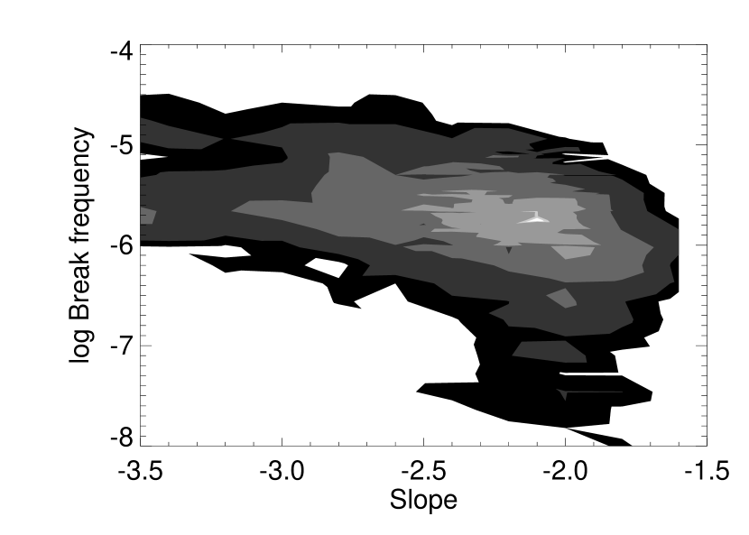
Figure 6: Confidence contours for a broken power law model with low frequency slope of $-1.2$. Contours are at 5, 10, 25, 50, and 75% probability of acceptance. Maximum confidence of 84.5% occurs at a high-frequency slope of $-2.1$ and a break frequency of $\log\nu_{\rm b}=-5.75$ Hz.

Figure 5 shows the observed PDS fitted with the best-fit broken power law model. The best fit parameters show a low-frequency slope of $\alpha_{\rm L}=-1.2$, high-frequency slope $\alpha_{\rm H}=-2.1\pm 0.4$, with a break at a frequency of $\log\nu_{\rm b}=-5.75\pm 0.43$ Hz, or a timescale of $6.51^{+11.0}_{-4.1}$ days. The probability of acceptance of this model is 84.5%. Figure 6 shows confidence contours for variations in the break frequency and high frequency slope. Error bars for the slope and break were obtained by taking a 1-dimensional slice through the confidence contours at the best-fit value, fitting the contours with a Gaussian and finding the standard deviation.

5.3 Doubly-Broken Power Law

Given that the low/hard state seen in BHXRBs shows two break frequencies, we also model the PDS of 3C 120 with a doubly broken power law. For computational efficiency, the slopes were fixed at values of $0$, $-1$, and $-2$, similar to that seen in Cygnus X-1 (Revnivtsev et al. 2000). The low frequency break was allowed to vary from $\log\nu_{\rm b,lo}=-9.0$ to $-5.5$, and the high frequency $\log\nu_{\rm b,hi}$ allowed to vary between 5 and 10,000 times greater than the low-frequency break.

A best fit was obtained at $\log\nu_{\rm b,lo}=-8.03$, $\log\nu_{\rm b,hi}=-5.83$, and a confidence level of 63.2%. The low frequency break is near the lowest measured frequency for our PDS, effectively turning the model into a singly-broken power law. Therefore we find no evidence for a doubly-broken power law in the PDS of 3C 120, with a singly-broken power law providing an adequate fit.

6 Discussion and Conclusions

We have shown that both X-ray and optical emission are highly variable over a period of several years, with fractional variabilities of 21.6% and 8.2% in the X-ray and optical, respectively (Markowitz & Edelson 2004). The variations are strongly correlated, with the X-ray variations leading the optical by 28 days. Additionally, the X-ray PDS is best fit by a broken power law, with a slope of $-1.2$ breaking to a slope of $-2.1$ above a break frequency of $\nu_{\rm b}=-5.75$ Hz, or 6.5 days.

Given that the PDS is best fit by a singly-broken power law, and does not show any signs of a double break, 3C 120 appears to fit well with the high/soft state power spectra found in most other AGN. This is appropriate, given the moderately high accretion rate of 30% Eddington for this object (Ogle et al. 2005). The X-ray spectrum is also relatively steep, with an average photon index of $\Gamma=1.8$ during our long-term monitoring, similar to the values of $\Gamma=2-3$ seen in high/soft state BHXRBs.

Using the fundamental plane of AGN variability (McHardy et al. 2006), we can investigate whether the break timescale measured for 3C 120 fits with a relation based on radio-quiet objects. The expected break timescale $T_{\rm B}$ is:

$$\log T_{\rm B}=2.1\log M_{\rm BH}-0.98\log L_{\rm Bol}-2.32$$

where $M_{\rm BH}$ is the mass of the black hole in units of $10^{6}\mbox{M}_{\odot}$, and $L_{\rm Bol}$ is the bolometric luminosity in units of $10^{44}$ erg/s. For 3C 120, $L_{\rm Bol}=21.87$ (Woo & Urry 2002), and $M_{\rm BH}=50^{+108}_{-18}$, as measured by Vestergaard & Peterson (2006) using reverberation mapping in the optical and UV. Using these values, we would expect to find a break at a timescale of $T_{\rm B}=0.86^{+8.78}_{-0.52}$ days, with the errors based on the large uncertainty in the mass. Therefore our measured break timescale agrees well with the prediction based on the fundamental variability plane, within the errors on both the mass and our measured break.

We can also check the relationship between H$\beta$ FWHM and $T_{\rm B}$ for 3C 120. This relationship is given by:

$$\log T_{\rm B}=4.2\log\rm{H}_{\beta,FWHM}-14.43$$

where $\rm{H}_{\beta,FWHM}$ is in units of km/s (McHardy et al. 2006). For 3C 120, Marziani et al. (2003) measured a FWHM of 2328 km/s. This gives us a predicted break timescale of 0.51 days, different by a factor of $\sim 2$ from the mass/luminosity scaling relationship, and different by a factor of $\sim 13$ from our actual measured value. The $H\beta-T_{\rm B}$ relationship is based on a sample of radio-quiet objects. Given that 3C 120 is radio loud, with a superluminal jet, the broad-line region may not share the same characteristics as a radio-quiet object. More observations of radio-loud AGN are needed to determine if a separate $H\beta-T_{\rm B}$ relationship exists for these objects.

Given that the X-ray behavior of this object appears similar to that from radio-quiet Seyfert galaxies, we can examine whether the X-ray emission comes from the jet, or from a source in/near the accretion disk. As noted by Ogle et al. (2005), although 2 X-ray sources are coincident with the positions of radio lobes, they contribute $<5$% of the overall X-ray flux.

Closer to the nucleus, we can use spectroscopy to determine how much of the flux originates in the jet. Ballantyne et al. (2004) have analyzed a 127 ks XMM/Newton observation of 3C 120. They find a neutral Fe K$\alpha$ line with an equivalent width of 53 eV. Kataoka et al. (2007) find evidence for a relativistically broadened line using Suzaku. The strength of the narrow Fe K$\alpha$ line indicates that the majority of the X-ray emission has its origin in an unbeamed source, such as the accretion disk or corona, as opposed to the jet. If the X-ray flux were beamed within a narrow cone, reflection would be unlikely. Ogle et al. (2005) find a half-opening angle for the continuum of $>50^{\circ}$, indicating the narrow jet is not responsible for the X-ray emission.

If the X-ray emission originates near the accretion disk, then where does the 28 day X-ray to optical lag arise from? Low polarization in the optical ($\sim 0.3$%, consistent with interstellar dust) indicates that the emission is not associated with the jet. Such a lag is also too large to arise from light travel time between different regions in the accretion disk, however the communication between X-ray and optical regions may propagate at sub-light speeds. A more complete optical light curve may give a more precise value of the delay, to confirm the result and better specify the required propagation speed of the variations.

Table 1: Summary of Observations

Duration	Start	End	T	$\Delta$T
Long	52335.42	54114.39	1779	2.33d
Medium	54054.66	54114.39	60	6h
Short	52622.39	52631.48	9.09	1000s
Optical	53248.73	54110.54	862	2.33d

Figure 1: RXTE 2–20 keV light curves for long (top), medium (middle), and short (bottom) timescales.

Figure 2: Optical R-band (top) and X-ray (bottom) light curves.

Figure 3: Discrete correlation function for X-ray and optical light curves. Positive lag indicates X-ray emission leading the optical. Dashed line shows a best-fit Gaussian curve, with centroid of +28 days. See text for a discussion of errors.

Figure 4: Histogram showing cross-correlation lag centroid versus number of simulation results yielding that lag for the FR/RSS method. Bin width is 1 day. Median result occurs at a lag of 28.73 days, with uncertainties of $+\Delta\tau_{68}=6.19$ and $-\Delta\tau_{68}=5.87$ days.

Figure 5: Observed PDS for long, medium, and short light curves represented by solid, dotted, and dashed lines, respectively. Monte Carlo simulations for each light curve are represented by diamonds, squares, and triangles with error bars. Best fit occurs with the low frequency slope fixed at $-1.2$, high frequency slope of $-2.1$, and a break frequency of $\log\nu_{\rm b}=-5.75$ Hz, with a probability of acceptance of 84.5%.

References

- Ballantyne et al. (2004) Ballantyne, D. R., Fabian, A. C., & Iwasawa, K. 2004, MNRAS, 354, 839
- Churazov et al. (2001) Churazov, E., Gilfanov, M., & Revnivtsev, M. 2001, MNRAS, 321, 759
- Edelson & Nandra (1999) Edelson, R., & Nandra, K. 1999, ApJ, 514, 682
- Edelson & Krolik (1988) Edelson, R. A., & Krolik, J. H. 1988, ApJ, 333, 646
- Esin et al. (1997) Esin, A. A., McClintock, J. E., & Narayan, R. 1997, ApJ, 489, 865
- Forman et al. (1978) Forman, W., Jones, C., Cominsky, L., Julien, P., Murray, S., Peters, G., Tananbaum, H., & Giacconi, R. 1978, ApJS, 38, 357
- French & Miller (1980) French, H. B., & Miller, J. S. 1980, PASP, 92, 753
- Haardt & Maraschi (1991) Haardt, F., & Maraschi, L. 1991, ApJ, 380, L51
- Haardt & Maraschi (1993) —. 1993, ApJ, 413, 507
- Kataoka et al. (2007) Kataoka, J., Reeves, J. N., Iwasawa, K., Markowitz, A. G., Mushotzky, R. F., Arimoto, M., Takahashi, T., Tsubuku, Y., Ushio, M., Watanabe, S., Gallo, L. C., Madejski, G. M., Terashima, Y., Isobe, N., Tashiro, M. S., & Kohmura, T. 2007, PASJ, 59, 279
- Lawrence & Papadakis (1993) Lawrence, A., & Papadakis, I. 1993, ApJ, 414, L85
- Maoz & Netzer (1989) Maoz, D., & Netzer, H. 1989, MNRAS, 236, 21
- Markowitz & Edelson (2004) Markowitz, A., & Edelson, R. 2004, ApJ, 617, 939
- Markowitz et al. (2003) Markowitz, A., Edelson, R., Vaughan, S., Uttley, P., George, I. M., Griffiths, R. E., Kaspi, S., Lawrence, A., McHardy, I., Nandra, K., Pounds, K., Reeves, J., Schurch, N., & Warwick, R. 2003, ApJ, 593, 96
- Marscher et al. (2002) Marscher, A. P., Jorstad, S. G., Gómez, J.-L., Aller, M. F., Teräsranta, H., Lister, M. L., & Stirling, A. M. 2002, Nature, 417, 625
- Marziani et al. (2003) Marziani, P., Sulentic, J. W., Zamanov, R., Calvani, M., Dultzin-Hacyan, D., Bachev, R., & Zwitter, T. 2003, ApJS, 145, 199
- McHardy & Czerny (1987) McHardy, I., & Czerny, B. 1987, Nature, 325, 696
- McHardy et al. (2007) McHardy, I. M., Arévalo, P., Uttley, P., Papadakis, I. E., Summons, D. P., Brinkmann, W., & Page, M. J. 2007, MNRAS, 382, 985
- McHardy et al. (2006) McHardy, I. M., Koerding, E., Knigge, C., Uttley, P., & Fender, R. P. 2006, Nature, 444, 730
- McHardy et al. (2004) McHardy, I. M., Papadakis, I. E., Uttley, P., Page, M. J., & Mason, K. O. 2004, MNRAS, 348, 783
- Miyamoto et al. (1991) Miyamoto, S., Kimura, K., Kitamoto, S., Dotani, T., & Ebisawa, K. 1991, ApJ, 383, 784
- Ogle et al. (2005) Ogle, P. M., Davis, S. W., Antonucci, R. R. J., Colbert, J. W., Malkan, M. A., Page, M. J., Sasseen, T. P., & Tornikoski, M. 2005, ApJ, 618, 139
- Papadakis & Lawrence (1993) Papadakis, I. E., & Lawrence, A. 1993, MNRAS, 261, 612
- Papadakis & Lawrence (1995) —. 1995, MNRAS, 272, 161
- Peterson et al. (1998) Peterson, B. M., Wanders, I., Horne, K., Collier, S., Alexander, T., Kaspi, S., & Maoz, D. 1998, PASP, 110, 660
- Revnivtsev et al. (2000) Revnivtsev, M., Gilfanov, M., & Churazov, E. 2000, A&A, 363, 1013
- Timmer & Koenig (1995) Timmer, J., & Koenig, M. 1995, A&A, 300, 707
- Uttley et al. (2003) Uttley, P., Edelson, R., McHardy, I. M., Peterson, B. M., & Markowitz, A. 2003, ApJ, 584, L53
- Uttley et al. (2002) Uttley, P., McHardy, I. M., & Papadakis, I. E. 2002, MNRAS, 332, 231
- Vestergaard & Peterson (2006) Vestergaard, M., & Peterson, B. M. 2006, ApJ, 641, 689
- Walker et al. (1982) Walker, R. C., Seielstad, G. A., Simon, R. S., Unwin, S. C., Cohen, M. H., Pearson, T. J., & Linfield, R. P. 1982, ApJ, 257, 56
- Webb et al. (1988) Webb, J. R., Smith, A. G., Leacock, R. J., Fitzgibbons, G. L., Gombola, P. P., & Shepherd, D. W. 1988, AJ, 95, 374
- White & Peterson (1994) White, R. J., & Peterson, B. M. 1994, PASP, 106, 879
- Woo & Urry (2002) Woo, J.-H., & Urry, C. M. 2002, ApJ, 579, 530