Kondo regime in triangular arrangements of quantum dots: Molecular orbitals, interference and contact effects

Abstract

Transport properties of an interacting triple quantum dot system coupled to three leads in a triangular geometry has been studied in the Kondo regime. Applying mean-field finite-U slave boson and embedded cluster approximations to the calculation of transport properties unveils a set of rich features associated to the high symmetry of this system. Results using both calculation techniques yield excellent overall agreement and provide additional insights into the physical behavior of this interesting geometry. In the case when just two current leads are connected to the three-dot system, interference effects between degenerate molecular orbitals are found to strongly affect the overall conductance. An $S=1$ Kondo effect is also shown to appear for the perfect equilateral triangle symmetry. The introduction of a third current lead results in an ‘amplitude leakage’ phenomenon, akin to that appearing in beam splitters, which alters the interference effects and the overall conductance through the system.

I Introduction

One of the most important and exciting aspects of molecular physics nowadays is the study of electronic transport properties of natural and/or fabricated structures at the nanoscopic scale. In nature, molecules can couple to the external environment (electron reservoirs) through extended orbitals, which permit conduction electrons to hop in and out of the molecule. Fabricated molecules can be made by coupled quantum dots (QDs) with discrete energy levels. kouwenhoven ; bednarek ; heath Depending upon the strength of the coupling between the QDs, they can behave as a molecule with extended orbitals, which can further couple to external electron reservoirs. The confinement of electrons inside this artificial ‘molecule’ produces strong Coulomb interactions,ramirez which may give rise under suitable conditions to Kondo physics for temperatures below a characteristic crossover temperature, the Kondo temperature, $T_{K}$.hewson ; pustilnik ; izumida In the simplest picture of this regime, for $T\ll T_{\rm K}$, the system forms a singlet state, created by the screening of the localized spin by the conduction electrons in the external reservoir. Since its first observation in QDs in 1998,david-nature the attention generated by the Kondo effect in these structures has led to an explosion in experiments and theory. For example, multiple QD systems have become platforms for the theoretical and experimental development of sophisticated arrangements in order to access the rich phenomenology of the Kondo problem, including non-Fermi-liquid behavior and quantum critical points.Potok

In this paper, we study the transport properties of a triple quantum dot (TQD) system in the ‘molecular regime’ [with strong interdot couplings; see Fig. 1(a)] in two distinct situations: Firstly, just two QDs are attached to independent electron reservoirs. Secondly, each QD is connected to an independent electron reservoir. In the latter case, we focus our attention on the conductance of the system through two of the three terminals (the same two used to measure conductance in the first case). We are particularly interested in understanding interference effects, especially the role played by the third lead in the propagation of electrons along the different trajectories.

Despite significant advances in the understanding of Kondo physics in doublemeir ; vernek ; cornaglia ; jeong ; busser and triplezitko2 ; jiang ; lobos ; kuzmenko1 ; zitko1 ; zitko1b QD structures made in the last few years, there are still important aspects of the problem which deserve to be studied in detail. For example, based on a suggestion by Zarand et al.,zarand one may ask if an SU(4) Kondo regime may be experimentally attained in a TQD geometry. In addition, the unprecedented control of parameters in these multi-dot structures opens the possibility of observing quantum critical points and their associated non-Fermi-liquid ground states. Although many of these have been theoretically identified, the very demanding experimental constraints required have resulted in only a few successful experimental realizations.Potok Further motivation to study TQD systems comes from the proposal by Saraga and Loss that these structures could be used to produce spatially separated currents of spin-entangled electrons.loss Experimentally, however, only few groups have reported work in these systems.gaudreau ; vidan ; rogge Most of these studies have been in the Coulomb blockade regime, and one of the works reports that a TQD device can act as a molecular rectifier.vidan

Žitko and Bonc̆azitko1 have recently studied theoretically a TQD system connected in series to two leads. They have found that for a certain range of inter-dot hopping parameters the system crosses over from a Fermi-liquid to a non-Fermi-liquid regime in a wide interval of temperatures. In a subsequent paper,zitko1b using the numerical renormalization group (NRG), these authors analyze a large number of phases for a system similar to the one we discuss in this paper. Notice, nevertheless, that there are important differences between their system and ours: The majority of the phases analyzed in detail in Ref. zitko1b, use a Kondo Hamiltonian for the dots. In that case, a crossover was predicted between the two-impurity and the two-channel Kondo-model non-Fermi-liquid fixed points. Their analysis of Anderson-impurity QDs brings their work closer to ours. However, they restrict their study mainly to regimes where the inter-dot hoppings are considerably smaller than the coupling to the leads, which is exactly the opposite regime we treat in our work. In addition, they only analyze results close to half-filling, while we consider all fillings. Finally, and more importantly, they did not analyze the very important influence of the third contact, which is one of the important results of the work we report here.

The physics of this arrangement of QDs has also been the subject of other theoretical works.lobos ; ingersent1 ; kuzmenko ; kikoin ; avishai ; sakano ; emary In particular, a situation where the system may present interesting, but rather complicated behavior, is in the fully symmetric case, i.e., when all inter-dot hoppings are the same and each QD is equally connected to an independent conducting band (in that case, the system has equilateral triangle symmetry). It is reasonable then, if the inter-dot hoppings are much smaller than the intra-dot Coulomb repulsion, to expect the TQD system to present a spin frustrated regime, as anti-ferromagnetic arrangement between electrons sitting in different QDs is not possible. Indeed, through the use of conformal field theory and NRG calculations, Ingersent et al. were able to characterize a novel, stable, frustration-induced non-Fermi-liquid phase for a three-impurity Kondo model.ingersent1 It should be noted that this is not the regime treated in the current work. Here, we concentrate in the regime where the inter-dot hoppings are of the same order of magnitude as the intra-dot Coulomb repulsion, and always larger than the coupling to the leads (the ‘molecular regime’).

Considering this rich theoretical context, it is important for our objectives to be clearly spelled out. They are three-fold: First, since it is important from an experimental point of view to analyze the charge fluctuations in the QDs as a function of the gate potential, and as most of the previous work mentioned above uses the Kondo model to represent the QDs, we will model the system using the Anderson impurity model to describe each quantum dot. Second, we carefully analyze the conductance vs. gate potential results in a regime where the inter-dot couplings are larger than the coupling to the leads, i.e., in the molecular regime. Although this regime excludes other interesting phases in this system analyzed before,zitko1b we believe that the molecular regime can be experimentally more accessible and therefore very relevant. Third, we analyze in detail the effects created by the introduction of a third electron reservoir, which is connected to the ‘free’ QD, i.e., the QD which is not connected to either of the reservoirs used to measure the conductance.

We study this system by calculating the appropriate propagators to obtain the charge, the local density of states at the dots, and the conductance, using two different approaches: a finite-U slave boson formalism developed in the mean-field approximation (FUSBMF),kotliar and the Embedded Cluster Approximation (ECA),ferrari99 ; davidovich where one diagonalizes a small cluster containing the dots, and then embeds it into the leads through a Dyson equation. These two completely different approaches provide a similar description of the physics of the TQD structure. Note that some of the results shown here were obtained using a recent variant of the ECA method, the Logarithmic-Discretization Embedded Cluster Approximation (LDECA).number3 In this variant, the non-interacting electron band is discretized logarithmically (a la NRG), which leads to much faster convergence with cluster size. The band discretization provided by LDECA is necessary in two circumstances: i) When finite-size effects preclude ECA from converging to the correct ground state, or when that convergence is too slow; and ii) When one wants to calculate quantitatively accurate local density of states (LDOS). We will clearly indicate when either method (ECA or LDECA) is used.

This paper is organized as follows: In section II, we specify the model used to represent the TQD and we briefly describe the numerical methods used (FUSBMF, ECA, and LDECA). The results obtained for the case where the TQD is coupled to two reservoirs are discussed in section III. The change in the transport properties caused by the introduction of a third lead attached to the TQD is discussed in section IV. Finally, in section V, we present the conclusions.

II TQD model and numerical methods

The TQD system studied in this work is schematically represented in Fig. 1(a).

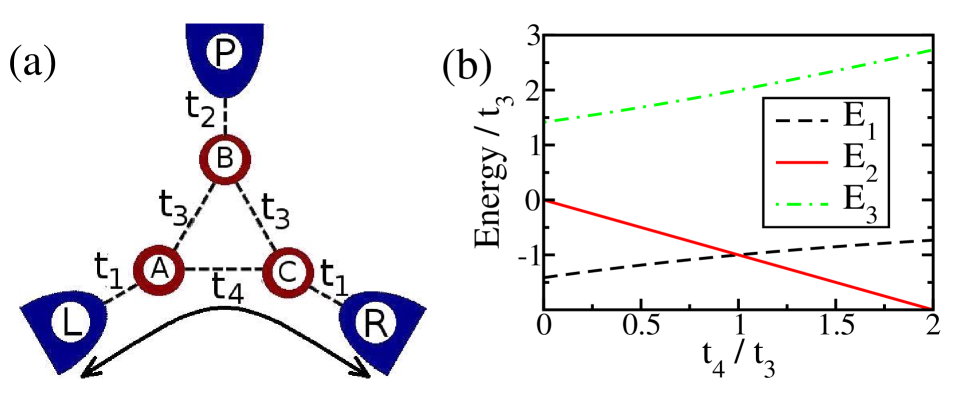
Figure 1: (color online) (a) Schematic representation of triple quantum dot system coupled to leads. As indicated by the arrows, we will calculate the conductance between the left (L) and right (R) contacts. (b) Energy diagram (in units of $t_{3}$) for the molecular orbitals [as defined in Eqs. (5)] as function of $t_{4}/t_{3}$.

The full Hamiltonian can be written as

$$H=H_{QDs}+H_{leads}+H_{QDs-leads},$$ (1)

where $H_{QDs}$ describes the isolated TQD system, $H_{leads}$ the two (or three) independent leads and $H_{QDs-leads}$ establishes the contacts between the dots and the leads. Explicitly, we have

$$H_{QDs} = \sum_{i=A,B,C\atop\sigma}V_{gi}d^{\dagger}_{i\sigma}d_{i\sigma}+U\sum_{i=A,B,C}n_{i\uparrow}n_{i\downarrow}$$ (2)

$$+\sum_{\sigma}\left[t_{3}(d^{\dagger}_{A\sigma}d_{B\sigma}+d^{\dagger}_{B\sigma}d_{C\sigma})+t_{4}d^{\dagger}_{A\sigma}d_{C\sigma}\right.$$

$$\left.+~{}{\rm H.c.}\right],$$

where $d^{\dagger}_{i\sigma}$ ($d_{i\sigma}$) creates (annihilates) an electron with spin $\sigma$ in the $i^{th}$ QD and energy controlled by the gate potential $V_{gi}$, $n_{i\sigma}=d^{\dagger}_{i\sigma}d_{i\sigma}$ is the occupation number operator, and $U$ is the Coulomb repulsion energy for double occupancy in a QD. The leads, modeled as semi-infinite chains, are represented by the Hamiltonian,

$$H_{leads}=t\sum_{i=1\atop{\gamma=L,R,P\atop\sigma}}^{\infty}\left[c^{\dagger}_{i_{\gamma}\sigma}c_{(i_{\gamma}+1)\sigma}+~{}{\rm H.c.}\right],$$ (3)

where $c^{\dagger}_{i_{\gamma}\sigma}$ ($c_{i_{\gamma}\sigma}$) creates (annihilates) an electron with spin $\sigma$ in the $i^{th}$ site of the $\gamma^{th}$ lead, and $t$ is the kinetic hopping between first neighbor sites. Finally, the contacts between the QDs and the leads are established by the Hamiltonian

$$H_{QDs-leads} = \sum_{\sigma}\left[t_{1}(d^{\dagger}_{A\sigma}c_{1_{L}\sigma}+d^{\dagger}_{C\sigma}c_{1_{R}\sigma})\right.$$ (4)

$$\left.+~{}t_{2}d^{\dagger}_{B\sigma}c_{1_{P}\sigma}+~{}{\rm H.c.}\right],$$

where $c_{1_{\gamma}\sigma}$ ($\gamma=L,R,P$) annihilates an electron in the first site of the $\gamma^{th}$ lead. Note also that for all cases studied here, a left $\leftrightarrow$ right symmetry applies.

In order to gain some intuitive understanding of the TQD system, let us consider the non-interacting case first. Let us further assume that $t_{1}=t_{2}=0$, so that the QDs are completely disconnected from the current leads. This is the ‘atomic limit’ of the model and can be solved exactly. In that case, the Hamiltonian eigenvalues are ($V_{gi}=V_{g}$),

$$E_{1} = V_{g}+\frac{t_{4}}{2}-\frac{1}{2}\sqrt{t^{2}_{4}+8t^{2}_{3}}$$ (5a)

$$E_{2} = V_{g}-t_{4}$$ (5b)

$$E_{3} = V_{g}+\frac{t_{4}}{2}+\frac{1}{2}\sqrt{t^{2}_{4}+8t^{2}_{3}}~{}.$$ (5c)

The un-normalized states are given by ([A,B,C]),

$$\mid\psi_{1}\rangle = [1,-\frac{t_{4}}{2t_{3}}-\frac{1}{2t_{3}}\sqrt{t_{4}^{2}+8t_{3}^{2}},1]$$ (6a)

$$\mid\psi_{2}\rangle = [-1,0,1]$$ (6b)

$$\mid\psi_{3}\rangle = [1,-\frac{t_{4}}{2t_{3}}+\frac{1}{2t_{3}}\sqrt{t_{4}^{2}+8t_{3}^{2}},1].$$ (6c)

Borrowing the terminology from molecular physics, orbitals $\mid\psi_{1}\rangle$, $\mid\psi_{2}\rangle$, and $\mid\psi_{3}\rangle$ will be denoted as bonding, non-bonding, and anti-bonding, from now on. For the particular case of $t_{4}=t_{3}\equiv t^{\prime\prime}$, $E_{1}=E_{2}=V_{g}-t^{\prime\prime}$ and $E_{3}=V_{g}+2t^{\prime\prime}$, the system has a doubly-degenerate state. In this case, the eigenvalues $E_{1}$, $E_{2}$, and $E_{3}$ correspond respectively to the orbitals

$$\mid\psi_{1}\rangle = \frac{1}{\sqrt{6}}[1,-2,1],$$ (7a)

$$\mid\psi_{2}\rangle = \frac{1}{\sqrt{2}}[-1,0,1],$$ (7b)

$$\mid\psi_{3}\rangle = \frac{1}{\sqrt{3}}[1,1,1].$$ (7c)

The degeneracy results from the symmetry of the system. In group theory language, it is associated to a two-dimensional irreducible representation of the $C_{3v}$ symmetry group. Note that, obviously, each orbital is also SU(2) symmetric, therefore, at zero field they are doubly degenerate regarding the spin orientation. For the full interacting Hamiltonian, these orbitals hybridize with the conduction electron band, renormalizing the eigenvalues. Although this is a simplified picture, it helps to understand the transport properties of the system. We will show that the degenerate orbitals have an important influence in the conductance of the interacting case.

In the interacting case, we are mainly interested in the Kondo regime and will study in detail how the symmetry (with its associated degeneracy) affects the transport properties. As mentioned above, the system is analyzed applying the FUSBMF, ECA, and LDECA methods. All three methods allow the calculation of the Green’s functions. We can easily calculate the charge at each dot and the total conductance of the system, which are respectively given by

$$\langle n_{i\sigma}\rangle=\frac{-1}{\pi}\int_{-\infty}^{\infty}{\rm Im}\{G^{\sigma}_{ii}(\omega)\}f(\omega)d\omega$$ (8)

and

$${\rm G_{T}}=4\pi^{2}t_{1}^{4}\rho_{R}(\epsilon_{F})\rho_{L}(\epsilon_{F})\mid G_{LR}(\epsilon_{F})\mid^{2},$$ (9)

where $G^{\sigma}_{ii}$ is the local Green’s function of the QDs, $f(\omega)$ is the Fermi function, $\rho_{L(R)}(\epsilon_{F})$ is the density of states of the left (right) lead’s first site and $G_{LR}(\epsilon_{F})$ is the Green’s function that propagates an electron from the left to the right lead, all calculated at the Fermi energy $\epsilon_{F}$. The expression for the conductance can be derived from the Keldysh formalismwingreen and is equivalent to the Landauer-Büttiker formula for the non-interacting case.

II.1 Finite-U slave bosons mean-field approximation

In the FUSBMF approach,kotliar one enlarges the Hilbert space by introducing a set of slave boson operators ${\hat{e}_{i}}$, $\hat{p}_{i\sigma}$ and $\hat{d}_{i}$ ($i=A,B,C$), and replace the creation ($d^{\dagger}_{i\sigma}$) and annihilation ($d_{i\sigma}$) operators in the Hamiltonian by $d^{\dagger}_{i\sigma}\hat{z}^{\dagger}_{i\sigma}$ and $\hat{z}_{i\sigma}d_{i\sigma}$, respectively. Following Kotliar and Rukenstein, the operator $\hat{z}$ takes the formkotliar

$$\hat{z}_{i\sigma}=[1-\hat{d}^{\dagger}_{i}\hat{d}_{i}-\hat{p}^{\dagger}_{i\sigma}\hat{p}_{i\sigma}]^{1/2}[\hat{e}^{\dagger}_{i}\hat{p}_{i\sigma}+\hat{p}^{\dagger}_{i\bar{\sigma}}\hat{d}_{i}]$$

$$\times[1-\hat{e}^{\dagger}_{i}\hat{e}_{i}-\hat{p}^{\dagger}_{i\bar{\sigma}}\hat{p}_{i\bar{\sigma}}]^{1/2}.$$ (10)

Notice that the bosonic operators $\hat{d}_{i}$ and $\hat{e}_{i}$ do not carry spin index. The enlarged Hilbert space is then restricted to the physically meaningful subspace by imposing the constraints

$$\hat{P}_{i}=\hat{e}^{\dagger}_{i}\hat{e}_{i}+\sum_{\sigma}\hat{p}^{\dagger}_{i\sigma}\hat{p}_{i\sigma}+\hat{d}^{\dagger}_{i}\hat{d}_{i}-1=0$$ (11)

and

$$\hat{Q}_{i\sigma}=d^{\dagger}_{i\sigma}d_{i\sigma}-\hat{p}^{\dagger}_{i\sigma}\hat{p}_{i\sigma}-\hat{d}^{\dagger}_{i}\hat{d}_{i}=0.$$ (12)

These constraints are enforced by introducing them into the Hamiltonian through Lagrange multipliers $\lambda^{(1)}_{i}$ and $\lambda^{(2)}_{i\sigma}$. The constraints (11) force the dots to have empty, single or double occupancy only, and (12) relates the boson to the fermion occupancy. In the mean-field approximation, the boson operators $\hat{e}_{i}$, $\hat{p}_{i\sigma}$ and $\hat{d}_{i}$ (and the corresponding Hermitian conjugates) are replaced by their thermodynamical expectation values $e_{i}\equiv\langle\hat{e}_{i}\rangle=\langle\hat{e}^{\dagger}_{i}\rangle$, $p_{i\sigma}\equiv\langle\hat{p}_{i\sigma}\rangle=\langle\hat{p}^{\dagger}_{i\sigma}\rangle$ and $d_{i}\equiv\langle\hat{d}_{i}\rangle=\langle\hat{d}^{\dagger}_{i}\rangle$. These expectation values, plus the Lagrange multipliers, constitute a set of parameters to be determined by minimizing the total energy $\langle H\rangle$. In principle, a set of seven selfconsistent parameters are needed for each dot. Although our system has three dots (which would require a total of 21 parameters), we take advantage of the symmetry of the configuration, since QDs $A$ and $C$ are symmetric with respect to $B$. Note that this symmetry imposes no additional constraint on the parameter values. In contrast with a previous implementation of this method, lobos our approach allows for a more complete and versatile description of the system in terms of its structural parameters. In particular, it can describe the transition from non-symmetrical to highly symmetrical regimes as the interdot parameters are changed.

In the mean-field approximation, we can obtain selfconsistent expressions for the Green’s functions. Then, using Eq. (8) and (9), we can calculate the charge at each dot and the conductance. We note that all the calculations with FUSBMF are implemented on the individual QD basis, while ECA and LDECA utilize the molecular basis.

II.2 Embedded Cluster Approximation

The ECA methodferrari99 ; davidovich relies on the numerical determination of the ground-state of a cluster with open boundary conditions. In the following, we briefly sketch details of the method.

The ECA method tackles the impurity problem in three steps. First, the infinite system is naturally cut into two parts: one part C (the cluster) contains the interacting region plus as many noninteracting sites of the leads as possible, and a second part R (the ‘rest’), consisting of semi-infinite chains positioned at left and right in relation to the cluster C. The number of sites in C is denoted by $N_{\mathrm{ED}}$. Second, Green’s functions for both parts are computed independently: current implementations of ECA utilize the Lanczos methodelbio to calculate the interacting Green’s function of the interacting region, while those of the part R, being noninteracting, can be computed exactly as well. In a final step, the artificially disconnected parts are reconnected by means of a Dyson equation, which dresses the interacting region’s Green’s function. This step, the actual embedding, is crucial for capturing the many-body physics associated with the Kondo effect. Moreover, although the clusters that can be solved exactly by means of a Lanczos routine are rather small, being of the order of $N_{\mathrm{ED}}\approx 12$ sites only, the embedding step successfully compensates for that by dressing the cluster Green’s function and effectively extending the many-body correlations, induced by the presence of the impurity, into the semi-infinite chains R. Obviously, strongly correlated regimes which depend on extremely low energy scales will be difficult to treat with the embedding procedure, although, as mentioned above, great progress has been made lately in this respect by introducing a logarithmic discretization procedure into the algorithm.number3

We now provide further detail on these steps. The Hamiltonians of the left and right semi-infinite, tight-binding chains, i.e., the noninteracting R part, are described by

$$H_{\rm sc-L} = -t\sum_{l=0,\sigma}^{-\infty}(c_{l\sigma}^{\dagger}c_{l-1\sigma}+~{}{\rm H.c.});$$

$$H_{\rm sc-R} = -t\sum_{l=N_{\mathrm{ED}}+1,\sigma}^{\infty}\-\-\-(c_{l\sigma}^{\dagger}c_{l+1\sigma}+~{}{\rm H.c.}),$$ (13)

where in this notation, the sites labeled by $i=1,\dots,N_{\mathrm{ED}}$ are inside the cluster C. The semi-infinite chains are connected to the cluster by the following term:

$$H_{\rm hy} = -V[c_{1\sigma}^{\dagger}c_{0\sigma}+c_{N_{\mathrm{ED}}\sigma}^{\dagger}c_{N_{\mathrm{ED}}+1\sigma}]+~{}{\rm H.c.},$$ (14)

where $V=t$ is the hopping in the broken link, connecting parts R and C, used in the embedding procedure. The Green’s function for the cluster C and for the semi-infinite chains are calculated at zero temperature. Fixing the number of particles $m$ and the $z$-axis projection of the total spin, $S_{\mathrm{total}}^{z}$, the ground state and the one-body propagators between all the clusters’ sites are calculated. For example, $g_{ij}^{(m,S^{z}_{total})}$, the undressed Green’s function for the cluster, propagates a particle between sites $i$ and $j$ inside the cluster. For the noninteracting, semi-infinite chains, the Green’s functions $g_{0}^{L}$ and $g_{N_{\mathrm{ED}}+1}^{R}$ at the sites $0$ and $N_{\mathrm{ED}}+1$, located at the extreme ends of the semi-infinite chains, at left and right to the cluster, can be easily calculated as well.

The Dyson equation to calculate the dressed Green’s function matrix elements $G^{(m,S_{\mathrm{total}}^{z})}_{i,j}$ can therefore be written as

$$G^{(m,S_{\mathrm{total}}^{z})}_{i,j} = g^{(m,S_{\mathrm{total}}^{z})}_{i,j}+g^{(m,S_{\mathrm{total}}^{z})}_{i,1}~{}V~{}G^{(m,S_{\mathrm{total}}^{z})}_{0,j}$$ (15)

$$+g^{(m,S_{\mathrm{total}}^{z})}_{i,N_{\mathrm{ED}}}~{}V~{}G^{(m,S_{\mathrm{total}}^{z})}_{N_{\mathrm{ED}}+1,j}$$

$$G^{(m,S_{\mathrm{total}}^{z})}_{0,j} = g_{0}^{L}~{}V~{}G^{(m,S_{\mathrm{total}}^{z})}_{1,j}$$ (16a)

$$G^{(m,S_{\mathrm{total}}^{z})}_{N_{\mathrm{ED}+1},j} = g_{N_{\mathrm{ED}}+1}^{R}~{}V~{}G^{(m,S_{\mathrm{total}}^{z})}_{N_{\mathrm{ED}},j}~{},$$ (16b)

where $V$, as mentioned above, is defined according to $H_{\rm hy}$. Eqs. (15) and (16) correspond to a chain approximation, where a locator-propagator diagrammatic expansion is used.anda81 ; metzner91 Note that ECA is exact in the case of $U=0$.

As mentioned before, the calculation of the propagator $g^{(m,S_{\mathrm{total}}^{z})}_{i,j}$ requires that fixed quantum numbers $m$ and $S_{\mathrm{total}}^{z}$ be used. However, after the embedding procedure, these quantum numbers are not good quantum numbers for the cluster anymore. Therefore, we have to incorporate processes into the ECA method that allow for charge fluctuations in the cluster C. To accommodate this requirement, different implementations of ECA have been devised, either by including different spin mixing strategiesferrari99 ; Fabian or by moving the Fermi energy of the leads.Willy

The spin mixing proceeds as follows. First, a cluster Green’s function with mixed charge is defined through

$$g^{(m+p,pS_{\mathrm{total}}^{z})}_{i,j}=(1-p)~{}g^{(m,0)}_{i,j}~{}+~{}p~{}g^{(m+1,S_{\mathrm{total}}^{z})}_{i,j},$$ (17)

where $p$ takes values between 0 and 1, and we are assuming that $m$ is even, in which case, the corresponding $S_{\mathrm{total}}^{z}=0$. In addition, note that for the cluster with charge $m+1$, $S_{\mathrm{total}}^{z}$ takes values $\pm 1/2$. The matrix element $g^{(m+p,pS_{\mathrm{total}}^{z})}_{i,j}$ corresponds to a situation where the charge in the cluster is between $m$ and $m+1$. The total charge in the cluster, before embedding, can be easily calculated as

$$q^{pS_{\mathrm{total}}^{z}}(p)=(1-p)m~{}+~{}p(m+1)=m+p.$$ (18)

Using Eqs. (15) and (16), the dressed Green’s function $\hat{G}^{(m+p,pS_{\mathrm{total}}^{z})}_{T}$ is obtained, and from this result, the charge in the cluster can be calculated:

$$Q^{pS_{\mathrm{total}}^{z}}(p)=\frac{-1}{\pi}\int_{-\infty}^{E_{F}}\mbox{Im}~{}\{\sum_{i}G^{(m+p,pS_{\mathrm{total}}^{z})}_{i,i}(\omega)\}d\omega\,,$$ (19)

where $E_{F}$ is the Fermi level. The value of $p$ is calculated self-consistently, satisfying

$$Q^{pS_{\mathrm{total}}^{z}}(p)=q^{pS_{\mathrm{total}}^{z}}(p).$$ (20)

If there is spin reversal symmetry, e.g., no magnetic field is applied, one can calculate the total Green’s function as

$$G_{i,j}^{T}(p)={1\over 2}\sum_{S_{\mathrm{total}}^{z}=\pm 1/2}G^{(m+p,pS_{\mathrm{total}}^{z})}_{i,j},$$ (21)

where $p$ satisfies Eq. (20). It is important to emphasize that the charge fluctuations taken into account by Eq. (17) are the ones between the cluster and the rest of the system, and not just the ones at the interacting region described by $H_{\rm int}$. The latter ones involve a very localized neighborhood of the dot and as a consequence, are typically already well described on isolated clusters only. Finally, it is noteworthy to point out that the self-consistent solution for the charge mixing parameter $p$ is either 0 or 1 in the Kondo regime, and in particular at the particle-hole symmetric point $V_{g}=-U/2$ (when analyzing a single-QD problem). Therefore, deep into the Kondo regime (i.e., at the particle-hole symmetric point), no charge mixing takes place at all, and very little charge mixing occurs in a window of gate potential around the particle-hole symmetric point. The parameter $p$ will start to take a finite value (note that $0\leq p\leq 1$) as the gate potential drives the system into the mixed-valence regime. The purpose of the charge mixing is thus mainly to smooth out the transition from an $N$ electron to an $N\pm 1$ electron ground state, which for the bare cluster is a crossover between ground states with different number of particles.

As mentioned above, some of the calculations were done using the LDECA method, which is an important extension of ECA. In it, to obtain a better description of the low energy physics of the system, the non-interacting band is logarithmically discretized. All the procedure described above remains the same, but the band discretization allows a much faster convergence to the Kondo regime with cluster size. A full description of LDECA can be found in Ref. number3, .

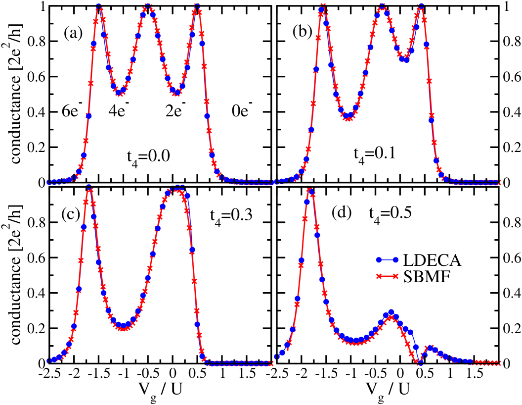
Figure 2: (color online) Conductance as function of gate potential, $V_{g}=V_{gA}=V_{gB}=V_{gC}$, for various values of $t_{4}$, as indicated in the panels. (Blue) solid dots indicate LDECA results for clusters with 11 sites; (red) ‘$\times$’ signs are FUSBMF results. Notice in panel (a), where $t_{4}=0$, that the number of electrons in the TQD system is indicated for each one of the valleys, where the Kondo effect is absent. The structure evolves from three to two peaks as the system goes from three dots in series [$t_{4}=0.0$, panel (a)], to isosceles [$t_{4}<t_{3}=0.5$, panels (b) and (c)], and finally to equilateral triangle symmetry [$t_{4}=t_{3}$, panel (d)]. For all panels, $U=1.0$, $t_{1}=0.45$, $t_{2}=0.0$, and $t_{3}=0.5$. The very small discrepancy between LDECA and FUSBMF in panel (d) comes from a finite-size effect in the LDECA results.

II.3 Numerical results

In order to study the conductance as a function of the parameters of the system, we use the leads’ hopping coupling $t$ as the energy unit ($t=1$), and set the Fermi energy to zero ($\epsilon_{F}=0$). All the results will be shown for zero-temperature. In the strong interdot coupling regime, i.e., $t_{3},t_{4}>t_{1},t_{2}$, the individual QDs levels mix into three molecular orbitals which are coupled to the leads. The energy of these orbitals can be controlled by gating the local energy states and by varying the hopping matrix elements ratio $t_{4}/t_{3}$ [see Fig. 1(b)]. Their widths depend upon the coupling to the conduction bands, i.e., $t_{1}$ and $t_{2}$. In order to study the contribution of each individual orbital to the conductance, we make them sufficiently far apart from each other. To do so, we take $t_{3}>t_{1},t_{2}$. In particular, in section III, we set $t_{1}=0.45$, $t_{2}=0.0$, $t_{3}=0.5$, and $U=1.0$ (which are the same parameters used in Ref. lobos, ), and in section IV we set $t_{1}=0.2$, $0.0\leq t_{2}\leq 0.2$, $t_{3}=0.4$, and $U=0.5$.note-molecular In section III, we vary $t_{4}$ to manipulate the symmetry of the system ($0.0\leq t_{4}/t_{3}\leq 1.0$). In section IV, besides the same variation of $t_{4}$ as in section III, we also analyze what is the effect of varying $t_{2}$ ($0.0\leq t_{2}/t_{1}\leq 1.0$), i.e., we verify what is the effect of adding a third lead [connected to QD B, see Fig. 1(a)] to the TQD system.

III TQD connected to two leads ($t_{2}=0$)

III.1 TQD in series ($t_{4}=0$)

Initially, taking advantage of the flexibility of the numerical methods used, we analyze the conductance when the three QDs are aligned in series ($t_{4}=0$) and coupled to two leads only (i.e., we make $t_{2}=0$). Fig. 2 shows the conductance as a function of the gate potential $V_{g}=V_{gA}=V_{gB}=V_{gC}$. In panel (a), for $t_{4}=0$ [(red) ‘$\times$’ signs indicate FUSBMF results, and (blue) solid dots display LDECA results], the three molecular orbitals are equally separated by an energy value proportional to $t_{3}$. As will be shown below, this originates from three Kondo peaks (occurring at different $V_{g}$ values) associated to each molecular orbital.

The $t_{4}=0$ case corresponds to the molecular regime reported in Ref. zitko2, (with, as mentioned above, $t_{3}>t_{1}$). For $t_{4}\neq 0$, the system transforms into a triangular configuration, which can be compared to the system studied in Ref. lobos, . In the first case ($t_{4}=0$, panel (a) in Fig. 2), the three peaks in the conductance occur at gate potential values where there is a change in the occupation of the different molecular orbitals. When the bonding orbital hosts one electron (for $V_{g}/U=0.5$), the system is in the Kondo regime and the characteristic Abrikosov-Suhl resonance of this regime creates a path for the electrons to cross from the left (L) to the right (R) lead [this will be more clearly demonstrated in Fig. 3(d)]. Decreasing $V_{g}$, we find a valley corresponding to the accommodation of a second electron in the bonding state, creating a singlet that destroys the Kondo effect. The middle peak corresponds to the presence of a third electron in the system, now siting in the non-bonding state, since the bonding state is full. Again, the conductance peak reflects the Kondo resonance at the Fermi level due to an unpaired electron that is anti-ferromagnetically correlated with the conduction electrons (see Fig. 3(b), and discussion below). The following valley and the third peak are a consequence of the suppression of the Kondo effect due to double occupation of the non-bonding orbital and the unpaired electron in the anti-bonding orbital, respectively. Finally, the final drop in the conductance results from the destruction of the Kondo effect due to the sixth electron entering into the system. The electron occupancies at the conductance valleys are indicated in panel (a).

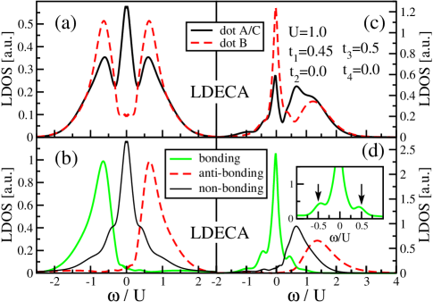
Figure 3: (color online) LDOS results using LDECA (9 sites) for $t_{1}=0.45$, $t_{2}=0.0$, $t_{3}=0.5$, $t_{4}=0.0$, and $U=1.0$. (a) and (c): LDOS for each QD. (a) and (b) are calculated at $V_{g}=-U/2$, while (c) and (d) at $V_{g}=U/2$. Note that, in (a), QDs A and C are in Kondo and QD B is not, while in (c) all dots participate in the Kondo effect. (b) and (d): LDOS for each molecular orbital. In (b), just the non-bonding orbital is in the Kondo state (dark (black) curve), as one can easily see its Kondo peak at $\omega=0.0$, while the bonding orbital (light (green) curve) is almost fully occupied (most of its LDOS is below the Fermi energy) and the anti-bonding orbital (dashed (red) curve) is almost empty (most of its LDOS is above the Fermi energy). In (d), it is now the bonding state that has a Kondo resonance, while the non-bonding and anti-bonding states are higher in energy. The inset shows a more detailed view of the Kondo peak for the bonding orbital, where the small LDOS peaks for the $\epsilon$ and $\epsilon+U$ states are indicated by arrows.

III.2 LDECA LDOS results for molecular orbitals ($t_{4}=0$)

Before analyzing the effect of introducing a finite $t_{4}$, we want to show LDOS results at the particle-hole symmetric point ($V_{g}=-U/2$) [Figs. 3(a) and (b)], and at $V_{g}=U/2$ [Figs. 3(c) and (d)] for the $t_{4}=0.0$ curve in Fig. 2(a). In the upper left panel in Fig. 3, we have the LDOS for each QD for $V_{g}=-U/2$. As expected, QDs A and C have the same LDOS (dark (black) solid curve), and the peak at $\omega=0$ is indicative that they participate in a Kondo effect. Indeed, a clear Kondo peak can be seen at the Fermi energy $E_{F}$ ($\omega=0.0$) for QDs A and C, while the LDOS for QD B has a gap at $E_{F}$ [dashed (red) curve in panel (a)]. This will be important later on to understand the results when the upper lead (P) is coupled to QD B (for finite $t_{2}$). The LDOS for the appropriate orbital states for this configuration ($t_{4}=0.0$, and $V_{g}=-U/2$) is shown in the lower left panel. The bonding orbital (gray (green) solid curve) has most of its LDOS below $E_{F}$, indicating that it is already almost fully occupied. In contrast, the anti-bonding orbital has, at this particular gate potential, most of its LDOS above $E_{F}$ and is therefore almost completely empty. The non-bonding orbital [which is an antisymmetrical combination of QDs A and C, only, see Eq. 6(b)] displays a Kondo peak at $E_{F}$, which is responsible for the unitary conductance seen for $t_{4}=0$ in Fig. 2(a) at $V_{g}=-U/2$. As to the rightmost peak in Fig. 2(a), notice, as can be seen in the upper right panel in Fig. 3(c), that all three QDs participate in the Kondo effect for $V_{g}=U/2$. In the lower right panel, one sees the LDOS for the orbital states, now indicating that the bonding state has a Kondo peak, while the other two orbitals are nearly empty.edge The inset shows details of the Kondo peak, for the bonding orbital, including the shorter peaks associated to $\epsilon$ and $\epsilon+U$, indicated by vertical arrows.

III.3 Finite $t_{4}$ and interference effects ($t_{4}\approx t_{3}$)

Now, as $t_{4}$ increases from $0$ to $0.5$ (panels (b) to (d) in Fig. 2), the bonding and non-bonding energies become closer to each other [see Eqs. (5)], and finally, become degenerate for $t_{4}=t_{3}=0.5$ [see Fig. 1(b)], when the system possesses an equilateral triangle symmetry. Note that the peaks in the conductance curves shown in Fig. 2, corresponding to the bonding (rightmost peak) and non-bonding (central peak) orbitals, merge into each other and the conductance decreases as $t_{4}\rightarrow t_{3}$. As shown above in Fig. 3, the LDOS of the molecular orbitals provides a more clear picture of the Kondo effect than the LDOS of each QD. For example, when $t_{4}=0$, the rightmost conductance peak in Fig. 2(a) can be directly associated to the Kondo peak in Fig. 3(d) (light (green) solid curve). As mentioned above, the molecular orbitals provide a natural description of the Kondo effect when the intra-dot hoppings are larger than the coupling to the leads.

In the same manner that the LDOS for each molecular orbital provides important insight into the conductance through the TQD system, one can define a ‘partial’ conductance ${\rm G_{i}}$ through each molecular orbital ‘${\rm i}$’ (${\rm i}=1,2,3$) in the following way (full details are given in Ref. interf, ):

$${\rm G_{i}}=\frac{e^{2}}{h}\left[t^{2}\tilde{g}_{l}t_{li}\rho(\epsilon_{F})\right]^{2}|G_{iR}(\epsilon_{F})|^{2}$$ (22)

where $\tilde{g}_{l}$ is the Green’s function in the first site of the left contact, $t_{li}$ is the coupling of the left lead with orbital $\mid\psi_{i}\rangle$, and $G_{iR}$ is the dressed Green’s function that moves an electron from $\mid\psi_{i}\rangle$ (where $i=1,2,3$) to the first site in the right contact. For $t_{4}\approx t_{3}$ and $V_{g}$ values such that mostly molecular orbitals $i=1,2$ are involved in the transport of charge (i.e., $-0.5\lesssim V_{g}/U\lesssim 0.5$, in panels (c) and (d) in Fig. 2), the total conductance ${\rm G_{T}}$ can be approximated by the equation

$${\rm G_{T}}\simeq{\rm G}_{12}={\rm G}_{1}+{\rm G}_{2}+2\sqrt{{\rm G}_{1}{\rm G}_{2}}\cos{\Delta\phi_{12}},$$ (23)

where

$$i\Delta\phi_{12}=\log\left\{\frac{G_{1R}}{G_{2R}}\frac{|G_{2R}|}{|G_{1R}|}\right\}$$ (24)

defines the phase-difference between a path that goes through orbital $\mid\psi_{1}\rangle$ and a path that goes through orbital $\mid\psi_{2}\rangle$. In the case where all three orbitals are contributing, a simple extension of these equations should be used, and it gives results exactly equal to the ones shown in Fig. 2. We should note that the ${\rm G_{i}}$ functions have a characteristic ‘width’ given by the coupling to the leads (and the weight of the orbital at the connecting dot), as well as a position dependence on $V_{g}$, as the energy of each orbital shifts with respect to the Fermi energy.

Equation (23) shows that when there is no energy overlap between $\mid\psi_{1}\rangle$ and $\mid\psi_{2}\rangle$ (therefore, no overlap between ${\rm G}_{1}$ and ${\rm G}_{2}$), which occurs when the corresponding orbitals are well separated in energy, the last interference term is zero, independently of the value of the phase difference. This is essentially the case for the conductance results for $t_{4}=0$ in Fig. 2(a). In this case, a simple sum of the partial conductances ${\rm G_{i}}$ through each molecular orbital is very similar (not shown) to the total conductance (and more so as the level separation increases for larger values of $t_{3}/t_{1}$). However, as shown next (see Fig. 4), once the molecular orbital levels start to overlap, the partial conductances ${\rm G_{i}}$ are no longer simply related to the total conductance, as the last term in Eq. (23) now plays a role, and its effect will obviously depend on the value of $\Delta\phi_{12}$. Therefore, the calculation of the partial conductances, and the phase difference of the corresponding Green’s functions, provides us with information about possible interference effects, as shown next. However, a word of caution is necessary. Since the simple addition of the partial conductances does not reproduce the total conductance when there is overlap between the molecular levels, we will not discuss the details of the ${\rm G_{i}}$’s, as they do not, by themselves, describe an experimentally observable quantity. Obviously, when there is no overlap, as is the case for $t_{3}\gg t_{1}$ and $t_{4}=0$ (see section IV), the partial conductance of each orbital is identical to the total conductance.

Figure 4 shows, in the main panel, LDECA partial conductances ${\rm G}_{1}$ (short-dashed (green) line) and ${\rm G}_{2}$ (thick solid (red) line), for molecular orbitals $\mid\psi_{1}\rangle$ and $\mid\psi_{2}\rangle$, respectively, the total conductance ${\rm G_{T}}$ (long-dashed (magenta) line), which takes in account all 3 orbitals, and ${\rm G}_{12}$ (thin solid (blue) line), as obtained through Eq. (23), where just orbitals $\mid\psi_{1}\rangle$ and $\mid\psi_{2}\rangle$ are taken in account. The reason why ${\rm G}_{12}$ and ${\rm G_{T}}$ are so similar is because orbital $\mid\psi_{3}\rangle$ is at a considerably higher energy in relation to the degenerate orbitals and therefore its contribution to the conductance for gate potential values around $V_{g}=0.5U$ is minimal. The phase difference $\Delta\phi_{12}$ (in units of $\pi$), as a function of gate potential, is shown in the inset. Note that the dip in the total conductance is related to a $V_{g}$ value where both partial conductances have the same value and $\Delta\phi_{12}=\pi$ (see inset).g0

The conductance features described in Fig. 2 are quite different from the results reported by the authors in Ref. lobos, . Although their system is the same as ours (and the parameters are the same), the authors of Ref. lobos, consider, for simplicity, a regime where the total molecular region is described by a single level impurity, which allowed them to reduce the number of bosons in the FUSBMF approximation. However, as our results show, the details of the internal structure of the molecule are essential to determine its transport properties. Notice that as $t_{4}$ increases, not only the peaks shift their positions but, as previously mentioned, also the structure of the peaks changes.

Panels (c) and (d) in Fig. 2 display slight quantitative discrepancies between LDECA and FUSBMF results, although the overall qualitative agreement between the two techniques is quite good. These discrepancies stem from finite-size effects in the LDECA results.finite LDECA calculations for increasingly larger exactly diagonalized clusters (not shown) indicate that the LDECA results gradually approach those from FUSBMF. This convergence becomes slower as $T_{K}$ decreases, but the LDECA and FUSBMF qualitatively agree for all regimes we checked.

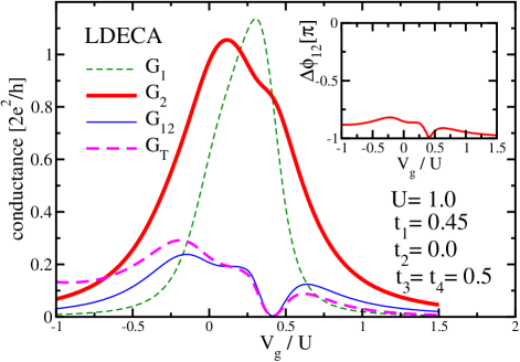
Figure 4: (color online) Detail of the conductance (calculated with LDECA – 11 sites) around the degenerate states $\mid\psi_{1}\rangle$ and $\mid\psi_{2}\rangle$: ${\rm G}_{1}$ (short dash (green) curve) and ${\rm G}_{2}$ (thick solid (red) curve), as defined in Eq. (22), ${\rm G}_{12}$ (thin solid (blue) curve), from Eq. (23), and the total conductance (involving all molecular orbitals) ${\rm G_{T}}$ (long dash (magenta) curve) from Eq. (9). The inset shows the phase difference between electrons propagating through molecular orbitals $\mid\psi_{1}\rangle$ and $\mid\psi_{2}\rangle$. See text for details.

Note that in the limit of strong coupling between dots A and C ($t_{4}\gg t_{3}$, and for $U>2t_{4}$), a two-stage Kondo regime (TSK) should be expected (at half-filling).cornaglia ; number3 In this regime, dot B is weakly coupled to the band through the Kondo resonances of quantum dots A and C, producing a second Kondo stage, with an exponentially smaller characteristic energy $T_{\rm TSK}\ll T_{\rm K}$. This special regime will be analyzed in a future work.

III.4 S=1 Kondo effect ($t_{4}=t_{3}$)

In addition to interference, the degeneracy (caused by symmetry) has an additional effect: it causes the two degenerate orbitals (when occupied by one electron each) to develop a ferromagnetic correlation. ferro Indeed, when the structure reaches the equilateral triangle symmetry (i.e., $t_{4}=t_{3}=0.5$), the two degenerate molecular orbitals are charged simultaneously. In this case, due to the Kondo correlation, the first two electrons enter in the system with parallel spins, and the system presents an $S=1$ Kondo effect. This can be quantitatively appreciated by calculating the total spin for the three QDs as a function of gate potential, as well as the individual occupancy of each of the three molecular orbitals. This is shown by the LDECA results in Fig. 5, where, together with the total conductance (long dash (magenta) curve), the charge occupancy for each of the molecular orbitals is shown (thin solid (purple) curve for orbital $\mid\psi_{1}\rangle$, dot-dashed (black) curve for orbital $\mid\psi_{2}\rangle$, and short dash (blue) curve for orbital $\mid\psi_{3}\rangle$), and the total spin in the three QDs (thick solid (green) curve). Notice that the occupancy dependence with $V_{g}$ for the two degenerate orbitals is not identical because they couple differently to the leads (orbital $\mid\psi_{2}\rangle$ couples more strongly than $\mid\psi_{1}\rangle$). As mentioned above, the maximum in the value of the total spin ($S_{T}\approx 0.7$, see thick solid (green) curve) occurs when there is approximately one electronnote-double in each of the degenerate orbitals, which couple through an effective ferromagnetic interaction.ferro (Note that a value of $S=1$ will not be obtained for such large ratios of hopping over Coulomb repulsion). This spin configuration reduces the ground state energy by Kondo correlating the total $S=1$ spin with the conduction electrons. In this region of gate potential, the system is in the Kondo regime, which provides a way for the electrons at the Fermi level to cross from QD A to QD C. However, having two interfering channels at their disposal, constructed from the two degenerate orbitals, the conductance (long dash (magenta) curve) possesses a very clear Fano-like antiresonance. For lower gate potential values ($V_{g}\approx-1.75$), only orbital $\mid\psi_{3}\rangle$ is involved in electron transport and therefore the conductance has the usual Lorentzian shape, with maximum value $G_{0}$, and $S_{T}\approx 0.4$.

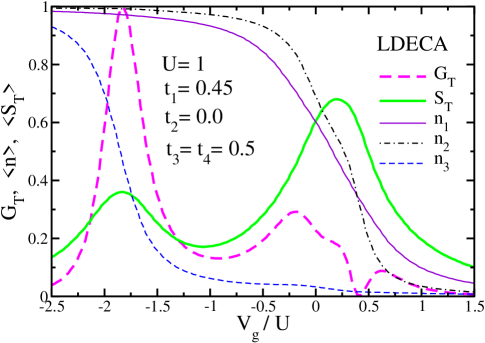
Figure 5: (color online) LDECA results (11 sites) for conductance (long dash (magenta) curve), same parameters as in Fig. 4. Charge per spin for each orbital [$\mid\psi_{1}\rangle$, thin solid (purple), $\mid\psi_{2}\rangle$, dot-dash (black), and $\mid\psi_{3}\rangle$, short dash (blue)], and total spin [thick solid (green)], as a function of gate potential. See text for details.

III.5 Deeper into Kondo and molecular regimes

As mentioned above, the parameters in this section were chosen to match those in Ref. lobos, . As expected, and clearly demonstrated by the LDOS’s in Fig. 3, the TQD system for these parameters seems to be closer to the intermediate valence regime than to the Kondo regime. Also, based on the fact that $t_{1}\approx t_{3}$, one may question if the molecular orbitals are really the most appropriate description of the single electron properties of the system. In view of that, in section IV, where the effect of introducing a third lead will be analyzed, the parameters will be changed so that the system will be deeper into the Kondo regime (with a larger $U/\Gamma$ than in the current section). To accomplish that, we will choose $U=0.5$ and $t_{1}=0.2$. In addition, in the next section, we will choose $t_{3}=0.4$ (with $0\leq t_{4}\leq t_{3}$), which brings the system more effectively into the molecular regime (as $t_{3}/t_{1}=2$). To illustrate both points, Fig. 6 shows the same LDOS results as in Fig. 3, but now for the new parameter set. It is apparent that the Kondo peaks for the new parameters are more well defined. For example, compare the dark solid (black) curves in panel (b) of both figures, which display the Kondo peak for the non-bonding orbital ($\mid\psi_{2}\rangle$). The peak in Fig. 6(b) clearly shows a sharper structure at the Fermi energy than the one in Fig. 3(b), indicating that this system is deeper into the Kondo regime. It is also apparent that the LDOS of the different molecular orbitals have much less overlap in Fig. 6, underscoring the fact that, for the parameters to be used in section IV, the molecular orbitals provide a more suitable description of the TQD system. Nonetheless, notice that the molecular orbitals provide an appropriate framework to understand the results presented in section III as well, as it is clear that Figs. 3 and 6 are qualitatively similar.

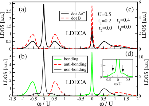
Figure 6: (color online) Same LDECA calculations (9 sites) as in Fig. 3, but now for $U=0.5$, $t_{1}=0.2$, $t_{2}=0.0$, $t_{3}=0.4$, and $t_{4}=0$. Note that the Kondo peaks are better defined than the ones in Fig. 3, as there is less overlap of the LDOS from different molecular orbitals, indicating that for these parameters the system is deeper into the Kondo and molecular regimes. Nonetheless, the qualitative similarities with Fig. 3 are evident, indicating that the molecular orbitals are appropriate for the description of the results in section III.

IV Loss of amplitude through a third lead

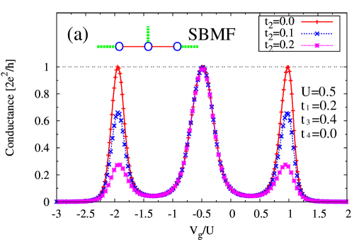
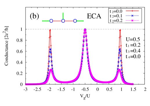
Figure 7: (color online) Conductance as function of gate potential, $V_{g}=V_{gA}=V_{gB}=V_{gC}$, for different values of $t_{2}$, showing the effect of the ‘amplitude loss’ due to the presence of the third lead. The other parameters are $U=0.5$, $t_{1}=0.2$, $t_{3}=0.4$, and $t_{4}=0$. Panels (a) and (b) refer to FUSBMF and ECA (6 sites) results, respectively.

In this section, as just mentioned, we use different parameters ($t_{1}=0.2$, $t_{3}=0.4$, $U=0.5$) from the ones used in section III. The objective is to have a larger value of $U/\Gamma$, and therefore move deeper into the Kondo regime and away from the intermediate valence.

Based on a comparison of the results in Fig. 2 with those in Figs. 7 and 8, a clear picture emerges of the effect of a third lead connected to QD B [see Fig. 1(a)]. Using the labels defined in Fig. 1(a) for the QDs, let us qualitatively describe how the coherent propagation of electrons is affected by the additional lead. Assume that an electron is traveling from the left into QD A. After arriving at QD A, the electronic wave splits into two: one travels via QD C, and the other via QD B. The latter portion, on reaching QD B, will be split into two again: one travels away through the upper lead, while the other travels via QD C. We can view this process of ‘electron loss’ through lead P (the ‘third’ lead) as being a process of ‘amplitude leakage’, like that occurring at a beam splitter. The remaining two traveling waves (traveling through the triangle, in the direction of QD C) are coherent and will interfere when they propagate out of the system through the right lead. It will be shown below that the introduction of lead P does not make the electron propagation incoherent, since the propagation through overlapping molecular orbital levels clearly shows signs of interference, the same way as observed for $t_{2}=0$, when the third lead is absent, as was discussed in Figs. 2 and 4. To analyze the results for conductance and LDOS, we use again the molecular orbital basis. The strategy for this analysis can be summarized by the following two observations: First, by analyzing the conductance through each molecular orbital, one realizes that the percentage of the traveling wave lost through lead P will depend on the coupling of each molecular orbital to it. This ‘loss’ through lead P will result in a lower partial conductance through the molecular orbital in question. Note that, for a fixed value of $t_{2}$, the coupling to lead P depends only on the coefficient of QD B in each molecular orbital, which varies with the ratio $t_{4}/t_{3}$. Second, if we assume that the transport through each molecular orbital is coherent (even after coupling QD B to lead P), the transport through two overlapping molecular orbital levels should give origin to interference effects, as in the case where lead P is not present (see section III). We will show evidence below that this is indeed the case.

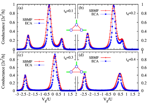
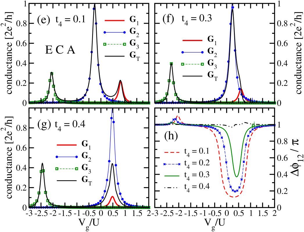
Figure 8: (color online) (a) to (d): Conductance as function of gate potential, $V_{g}=V_{gA}=V_{gB}=V_{gC}$, obtained with FUSBMF [‘+’ signs (red)] and ECA (6 sites) [stars (blue)] for several values of $t_{4}$. Panels (a), (b), (c) and (d) show how the peak structure evolves from three to two peaks as the system goes from isosceles to equilateral triangle symmetry [$t_{4}=t_{3}=0.4$, panel (d)]. For all panels, $U=0.5$, $t_{2}=t_{1}=0.2$, and $t_{3}=0.4$. Panels (e) to (g) show ECA (6 sites) results for the partial conductances ${\rm G_{i}}$ (${\rm G}_{1}$, thick solid (red) curve; ${\rm G}_{2}$, solid (blue) dots curve; ${\rm G}_{3}$, open squares (green) curve), together with the total conductance ${\rm G_{T}}$ (thin solid (black) curve). Panel (h) shows the evolution with $t_{4}$ of the phase difference $\Delta\phi_{12}$ between molecular orbitals $\mid\psi_{1}\rangle$ and $\mid\psi_{2}\rangle$, in units of $\pi$.

IV.1 TQD in series ($t_{4}=0$)

Before presenting the results, we should point out that most of the embedded cluster results in this section were obtained with ECA, not LDECA.note-ldos As will be seen below, in contrast to Fig. 2(d), where the LDECA results suffer from minor finite-size effects, no such effects were detected after the third lead is connected. The higher symmetry obtained when $t_{2}=t_{1}$ leads to no discernible finite-size effects for $t_{4}=t_{3}$. There are two main reasons for that. First, the third contact provides a way for the ‘frozen’ spin (present for $t_{2}=0$)finite to delocalize from QD B. Second, when $t_{4}=t_{3}$ and $t_{2}=t_{1}$, any net spin would be equally distributed among the three QDs, diminishing its ability to suppress the Kondo effect in an ECA calculation.Fabian

Let us start by turning on the connection of QD B to lead P, by varying $t_{2}$ from zero to $t_{1}=0.2$. To facilitate the analysis, we start with $t_{4}=0$ (three QDs in series, see Fig. 7). In this case, the molecular orbitals are:

$$\mid\psi_{1}\rangle = [1,-\sqrt{2},1]/2$$ (25a)

$$\mid\psi_{2}\rangle = [-1,0,1]/\sqrt{2}$$ (25b)

$$\mid\psi_{3}\rangle = [1,\sqrt{2},1]/2,$$ (25c)

with $E_{1}=V_{g}-\sqrt{2}t_{3}$, $E_{2}=V_{g}$, and $E_{3}=V_{g}+\sqrt{2}t_{3}$. Since state $\mid\psi_{2}\rangle$ does not involve QD B, the processes of wave-splitting and loss of amplitude of the propagating wave through lead P will not occur when $\mid\psi_{2}\rangle$ is the state near the Fermi energy (i.e., $V_{g}=-U/2$). This results in the partial conductance ${\rm G}_{2}$ through level $\mid\psi_{2}\rangle$ being unitary, i.e., ${\rm G}_{2}=G_{0}=2e^{2}/h$, for any value of $t_{2}$. This is clearly what happens to the central peak in Fig. 7, which is associated to the molecular orbital $\mid\psi_{2}\rangle$, as previously discussed in Figs. 2(a) and 3(b). The conductance through the other two molecular levels (rightmost and leftmost peaks in Fig. 7), as mentioned above, will depend on the weight of QD B in $\mid\psi_{1}\rangle$ and $\mid\psi_{3}\rangle$. Note that, as mentioned above, because of the choice of parameters ($t_{3}/t_{1}=2$), the total conductance is basically the direct sum of the partial conductances when $t_{4}=0.0$ (as there is minimal overlap between the molecular orbitals). For $t_{4}=0$ (see Eqs. 25 above), QD B has the same coefficient in $\mid\psi_{1}\rangle$ and $\mid\psi_{3}\rangle$, therefore ${\rm G}_{1}={\rm G}_{3}$ for any value of $t_{2}$ (see the identical leftmost and rightmost peaks in Fig. 7). The simultaneous and drastic decrease of ${\rm G}_{1}$ and ${\rm G}_{3}$ as $t_{2}$ increases comes from the increase of the coupling of QD B to lead P, which increases the amplitude loss through the third lead. Note the agreement between FUSBMF (top panel in Fig. 7), and ECA (bottom panel).noteconv

IV.2 Finite $t_{4}$

An interesting picture emerges for finite $t_{4}$. In Fig. 8, the top 4 panels show a comparison of conductance results calculated with FUSBMF (‘+’ (red) signs) and ECA [stars (blue)] for $t_{4}=0.1$, $0.2$, $0.3$, and $0.4$. The most salient feature in these results is the abrupt suppression of conductance when $t_{4}$ varies from 0.3 to 0.4. An explanation of this abrupt suppression is presented in three of the lower panels, which show ECA results for the total conductance (for $t_{4}=0.1$, $0.3$, and $0.4$, in panels (e), (f), and (g), respectively), as well as partial conductances through each molecular orbital. In addition, panel (h) shows phase difference results [see Eq. (24)] for paths going through either molecular orbital $\mid\psi_{1}\rangle$ or $\mid\psi_{2}\rangle$, for varying values of $t_{4}$.

As $t_{4}$ increases, the coefficient of QD B in $\mid\psi_{1}\rangle$ increases monotonically (in absolute value), until it reaches $-2/\sqrt{6}$ for $t_{4}=t_{3}$, while it decreases monotonically for orbital $\mid\psi_{3}\rangle$, reaching $1/\sqrt{3}$ for $t_{4}=t_{3}$ [see Eqs. (6) and (7)]. In accordance to that, ${\rm G}_{1}$ decreases as $t_{4}$ increases, while ${\rm G}_{3}$ increases, because of the associated changes in the coupling of states $\mid\psi_{1}\rangle$ and $\mid\psi_{3}\rangle$ to lead P: more coupling ($\mid\psi_{1}\rangle$), more ‘leakage’; less coupling ($\mid\psi_{3}\rangle$), less ‘leakage’. Note that, in panels (e) to (g) in Fig. 8, this is evident, as the solid (red) curve corresponds to ${\rm G}_{1}$ and the open squares (green) curve corresponds to ${\rm G}_{3}$. In addition, since molecular orbital $\mid\psi_{2}\rangle$ is independent of $t_{4}$ [see Eq. 6(b)], the maximum value of ${\rm G}_{2}$ (solid (blue) dots) is $G_{0}$ for all values of $t_{4}$ (no coupling of lead P to $\mid\psi_{2}\rangle$ results in no ‘leakage’). This can also be clearly seen in panels (e) to (g) of Fig. 8, where results for ${\rm G}_{2}$ are shown with solid dots (blue). Finally, as $t_{4}$ approaches $t_{3}$, molecular orbitals $\mid\psi_{1}\rangle$ and $\mid\psi_{2}\rangle$ approach each other [see Fig. 1(b)], allowing interference between them to strongly influence the transport properties of the system for $V_{g}$ values where these orbitals are close to the Fermi energy. It so happens that the phase difference between the paths through these two orbitals [as calculated in accordance to section III, Eq. (24), and shown in Fig. 8(h)], for the relevant values of $V_{g}$, changes from approximately zero (for $t_{4}=0.1$, dashed (red) curve) to $\pi$ (for $t_{4}=t_{3}=0.4$, double-dot-dash (black) curve). As discussed in section III, the interference will have noticeable effects only when the molecular orbitals $\mid\psi_{1}\rangle$ and $\mid\psi_{2}\rangle$ are close enough in energy (for $t_{4}\approx t_{3}$). At this point, the interference will be mostly destructive, as the phase difference is $\approx\pi$ (the resulting total conductance ${\rm G_{T}}$ is shown for all values of $t_{4}$ in panels (e) to (g) as a thin solid (black) curve). We see the abrupt suppression of the central peak (associated to ${\rm G}_{2}$), due to its interference with the right-side peak (associated to ${\rm G}_{1}$) for $t_{4}=t_{3}$ (see panel (g) in Fig. 8).

One may ask why the suppression of the conductance in Fig. 8(d) is less severe than the one in Fig. 2(d) [note that there are no Fano anti-resonances in Fig. 8(d)]. The reason is that, because of the presence of lead P, ${\rm G}_{1}$ is considerably less than the unitary conductance value $G_{0}$ [see thick solid (red) curve in Fig. 8(g)]. Therefore, destructive interference cannot be total (even if the phase difference is $\pi$), as ${\rm G}_{2}$ and ${\rm G}_{1}$ have widely different values. This is not the case in Fig. 4, where both partial conductances have similar values (being exactly the same at one $V_{g}$ value), as in that case lead P is not present.

The results just described for the conductance of the central peak ($\mid\psi_{2}\rangle$) in Fig. 7, where $t_{2}$ takes values $0$, $0.1$, and $0.2$, can also be understood in terms of the LDECA density of states. Figure 9 shows the LDOS for QDs A and C [panel (a)], and QD B [panel (b)], for $V_{g}=-U/2$ (corresponding to the central peak in Fig. 7). Notice that there is no sizable change in the value of the density of states at the Fermi energy ($\omega=0$), for any of the QDs, as $t_{2}$ varies. Since in this case the conductance is directly proportional to the density of states at the Fermi energy, this leads to a central peak in Fig. 7 that does not change with $t_{2}$. Obviously, this independence from $t_{2}$ comes from the fact that the density of states of QD B is very small in a broad interval around the Fermi energy when the charge transport occurs through orbital $\mid\psi_{2}\rangle$, resulting in lead P being effectively disconnected from the TQD for this value of $V_{g}$. Notice that as lead P couples to the other molecular orbitals ($\mid\psi_{1}\rangle$ and $\mid\psi_{3}\rangle$), there is no longer a simple proportionality relation between the LDOS and the conductance,leadP so that no simple direct connection can be made between the LDOS at the Fermi energy and the conductance (as was done in Fig. 3).

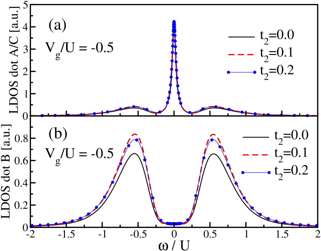
Figure 9: (color online) LDOS calculated using LDECA (6 sites) for $U=0.5$, $t_{1}=0.2$, $t_{3}=0.4$, $t_{4}=0$, and varying values of $t_{2}$, at the particle-hole symmetric point ($V_{g}/U=-0.5$). Panel (a) contains results for QDs A and C and panel (b) for QD B. In panel (a), it is evident that coupling QD B to lead P ($t_{2}=0.1$, dashed (red) curve, and $t_{2}=0.2$, solid (blue) dots curve) has no effect over the density of states of QDs A and C, as curves are indistinguishable from the $t_{2}=0$ case (solid (black) curve). Thus, the conductance does not change with $t_{2}$ (see Fig. 7). Note in panel (b) that QD B has no spectral weight at $\omega=0$ for any value of $t_{2}$, implying that when charge transport occurs through orbital $\mid\psi_{2}\rangle$, the conductance of the TQD is not affected by its coupling to lead P.

V Conclusions

We have studied the transport properties of a TQD in the molecular regime coupled to leads. By applying the FUSBMF, and the ECA and LDECA approaches, we have calculated the conductance of the TQD system for different symmetries and different configurations of the leads. For the two-leads case, we have calculated the conductance for both series and triangle configurations. In the series configuration, LDECA and FUSBMF results agree with each other and with the results for the molecular regime obtained in Ref. zitko1, , where the Kondo effect has been studied in detail. In the triangular symmetry, the quantitative results obtained by FUSBMF and LDECA differ slightly as the equilateral symmetry is approached, due to a finite-size effect in the relatively small clusters accessible to LDECA, although agreement is still very good [see Fig. 2(d)]. The suppression of conductance in the regime where approximately two electrons occupy the triangle was explained by LDECA as an interference effect between two degenerate molecular orbitals, utilizing the concept of partial conductance. In addition, our results for triangular symmetry differ from those presented recently in Ref. lobos, . We believe that the approach pursued here, where details of the internal structure of the interacting region of the system are taken fully into account, are very important to explain the conductance of the TQD system. In fact, our results show that changes in the internal couplings of the TQD dramatically change the features of the conductance. We also found that the degeneracy of the molecular orbitals at equilateral symmetry, when two electrons occupy the TQD, induces an effective ferromagnetic interaction between the spins localized in the interacting region,ferro leading to an $S=1$ Kondo effect.

In the TQD series configuration, our results show that the third lead produces a strong suppression in the bonding and anti-bonding orbital conductance peaks (Fig. 7). The non-bonding peak, however, remains unchanged, since this orbital does not have the appropriate symmetry to couple to lead P. This suppression of conductance can be seen as a ‘loss of amplitude’ through lead P, similar to the effect occurring with beam splitters in optics. If one thinks of the conductance in terms of transmission of waves through the interacting region, the introduction of lead P provides an additional transmission channel, which clearly affects the conductance between leads L and R. This ‘loss of amplitude’ idea is then used to understand the conductance results in the triangular symmetry. In particular, it explains why the interference effects seem less effective in suppressing the conductance in the equilateral symmetry (i.e., why no Fano anti-resonance occurs): the ‘loss of amplitude’ prevents the conductance through molecular orbital $\mid\psi_{1}\rangle$ from reaching the unitary limit, leading to a decrease in the destructive interference, as discussed in detail in Fig. 8. We should remark that the excellent overall quantitative agreement of results obtained with FUSBMF, ECA, and LDECAfinite ; noteconv (which rely on totally different approximations) makes our conclusions much more reliable and robust. Moreover, the combination of techniques allows a better insight into the physics of the different geometries.

- (1) L. Kouwenhoven, Science 268, 1440 (1995).
- (2) S. Bednarek, T. Chwiej, and J. Adamowski, Phys. Rev. B 67, 205316 (2003).
- (3) J. R. Heath and M. A. Ratner, Phys. Today 56, 43 (2003).
- (4) F. Ramirez, E. Cota, and S. E. Ulloa, Superlattices and Microstructures 20, 523 (1996).
- (5) A. C. Hewson The Kondo problem to heavy fermions (Cambridge University Press) (1993).
- (6) M. Pustilnik and L. I. Glazman, Phys. Rev. Lett. 87, 216601 (2001).
- (7) W. Izumida, O. Sakai, and Y. Shimizu, Physica B 261, 215 (1999).
- (8) D. Goldhaber-Gordon, H. Shtrikman, D. Mahalu, D. Abusch-Magder, U. Meirav, and M. A. Kastner, Nature 391, 156 (1998).
- (9) R. M. Potok, I. G. Rau, H. Shtrikman, Y. Oreg, and D. Goldhaber-Gordon, Nature 447, 167 (2007).
- (10) A. Georges and Y. Meir, Phys. Rev. Lett. 82, 3508 (1999).
- (11) E. Vernek, N. Sandler, S. E. Ulloa, and E. V. Anda, Phys. E 34, 608 (2006).
- (12) P. S. Cornaglia and D. R. Grempel, Phys. Rev. B 71, 075305 (2005)
- (13) H. Jeong, A. M. Chang, and M. R. Melloch, Science 293, 2221 (2001).
- (14) C. A. Büsser, E. V. Anda, A. L. Lima, M. A. Davidovich, and G. Chiappe, Phys. Rev. B 62, 9907 (2000).
- (15) R. Žitko and J. Bonča, A. Ramšak, and T. Rejec, Phys. Rev. B 73, 153307 (2006).
- (16) Z. T. Jiang, Q. F. Sun, and Y. P. Wang, Phys. Rev. B 72, 045332 (2005).
- (17) A. M. Lobos and A. A. Aligia, Phys. Rev. B 74, 165417 (2006).
- (18) T. Kuzmenko, K. Kikoin, and Y. Avishai, Europhys. Lett. 64, 218 (2003)
- (19) R. Žitko and J. Bonča, Phys. Rev. Lett. 98, 047203 (2007).
- (20) R. Žitko and J. Bonča, Phys. Rev. B 77, 245112 (2008).
- (21) G. Zarand, A. Brataas, and D. Goldhaber-Gordon, Solid State Commun. 126, 463 (2003).
- (22) D. S. Saraga and D. Loss, Phys. Rev. Lett. 90, 166803 (2003).
- (23) A. Vidan and R. M. Westervelt, App. Phys. Lett. 85, (16) 3202 (2004).
- (24) L. Gaudreau, S. A. Studenikin, A. S. Sachrajda, P. Zawadzki, A. Kam, J. Lapointe, M. Korkusinski, and P. Hawrylak, Phys. Rev. Lett. 97, 036807 (2006).
- (25) M. C. Rogge and R. J. Haug, Phys. Rev. B 77, 193306 (2008).
- (26) K. Ingersent, A. W. W. Ludwig, and I. Affleck, Phys. Rev Lett. 95, 257204 (2005).
- (27) T. Kuzmenko, K. Kikoin, and Y. Avishai, Phys. Rev. B 73, 255310 (2006).
- (28) K. Kikoin, T. Kuzmenko, and Y. Avishai, Phys. B 378-380, 906 (2006).
- (29) Y. Avishai, T. Kuzmenko, and K. Kikoin, Phys. E 29, 334 (2005).
- (30) R. Sakano, N. Kawakami, Phys. Rev. B 72, 084303 (2005).
- (31) C. Emary, Phys. Rev. B 76, 245319 (2007).
- (32) G. Kotliar and A. E. Ruckenstein, Phys. Rev. Lett. 57, 1362 (1986).
- (33) V. Ferrari, G. Chiappe, E. V. Anda, and M. A. Davidovich, Phys. Rev. Lett. 82, 5088 (1999).
- (34) M. A. Davidovich, E. V. Anda, C. A. Büsser, and G. Chiappe, Phys. Rev. B 65, 233310 (2002); E. V. Anda, C. A. Büsser, G. Chiappe, and M. A. Davidovich, Phys. Rev. B 66, 035307 (2002); G. B. Martins, C. A. Büsser, K. A. Al-Hassanieh, E. V. Anda, A. Moreo, and E. Dagotto, Phys. Rev. Lett. 96, 066802 (2006).
- (35) E. V. Anda, G. Chiappe, C. A. Büsser, M. A. Davidovich, G. B. Martins, F. Heidrich-Meisner, and E. Dagotto, Phys. Rev. B 70, 085308 (2008).
- (36) Y. Meir, N. S. Wingreen, and P. A. Lee, Phys. Rev. Lett. 66, 3048 (1991); E. V. Anda and F. Flores, J. Phys.: Condens. Matter 3, 9087 (1991).
- (37) E. Dagotto, Rev. Mod. Phys. 66, 763 (1994).
- (38) E. Anda, J. Phys. C 14, 1037 (1981).
- (39) W. Metzner, Phys. Rev. B 43, 8549 (1991).
- (40) F. Heidrich-Meisner, G. B. Martins, C. A. Büsser, K. A. Al-Hassanieh, A. E. Feiguin, G. Chiappe, E. V. Anda, and E. Dagotto, cond-mat:0705.1801 (to appear in Eur. Phys. Journ. B).
- (41) G. Chiappe, E. Louis, E. V. Anda and J. A. Verges, Phys. Rev. B 71, 241405(R) (2005); J. M. Aguiar-Hualde, G. Chiappe, E. Louis and E. V. Anda, Phys. Rev. B 76, 155427 (2007).
- (42) Although some of the results presented in section III are for parameter values such that , we checked that the results are qualitatively similar to the ones obtained for . Therefore, one can be confident that the parameters used in section III reflect the molecular regime situation (see also section III-E).
- (43) As discussed in detail in Ref. number3, , the LDOS in an LDECA calculation is artificially distorted as one moves away from the Fermi energy (). This distortion is caused by the logarithmic discretization of the band, and results in an ‘unphysical’ broadening of the poles as increases, especially for the large value we consider. That is why one has LDOS values beyond the band edge (particularly for ) in Figs. 3(c) and 3(d). This distortion also appears in LDOS calculations using NRG for similar parameter sets [see R. Bulla, T. A. Costi, and T. Pruschke, Rev. Mod. Phys. 80, 395 (2008)].
- (44) C. A. Büsser, G. B. Martins, K. A. Al-Hassanieh, A. Moreo, and E. Dagotto, Phys. Rev. B 70, 245303 (2004).
- (45) Note that the partial conductances and in Fig. 4 have maximum values larger than the conductance quantum (). As alluded above, the partial conductances, when their associated molecular orbitals overlap with each other, cannot be independently measured, having therefore no physical significance by themselves, and therefore do not have to be . When the molecular orbital levels are well separated in energy (and therefore the partial conductances match the total (measured) conductance), then . For all cases, moreover, the total conductance , as one expects on physical grounds.
- (46) The origin of the finite size effect is an unfavorable geometry for small clusters for , which tends to ‘freeze’ a spin in QD B. This suppresses spin fluctuations, with a consequent suppression of the Kondo effect. For a comprehensive discussion of similar effects in different systems (using ECA and DMRG), see Ref. Fabian, .
- (47) When two electrons are each occupying orbitals and , for (see Fig. 5),note-double the hopping from one lead to the orbitals (and vice versa) is maximized when the spins of the electrons in the molecular orbitals and are parallel to each other, i.e., ferromagnetically correlated, generating an effective ferromagnetic interaction between the orbitals. See G. B. Martins, C. A. Büsser, K. A. Al-Hassanieh, A. Moreo, and E. Dagotto, Phys. Rev. Lett. 94, 026804 (2005) for a similar effect in a different system.
- (48) Note that results for in Fig. 5 have to be multiplied by 2 to account for different spin orientations.
- (49) Except, obviously, for the LDOS results, where LDECA was used with .
- (50) Although there is good qualitative agreement between FUSBMF and ECA in Fig. 7, the ECA conductance peaks are narrower. This arises from the fact that the clusters used for these calculations had just 6 sites, and therefore the results are not fully size-converged. The next cluster size available for this geometry contains 12 sites. Although feasible, ECA calculations for this cluster size consume considerably more CPU time.
- (51) To confirm this, a test for a simplified system containing a single-level QD with three leads shows that the conductance through two of the leads is not directly proportional to the LDOS at the QD.