Fractional multiplicative processes

Abstract.

Statistically self-similar measures on $[0,1]$ are limit of multiplicative cascades of random weights distributed on the $b$-adic subintervals of $[0,1]$. These weights are i.i.d, positive, and of expectation $1/b$. We extend these cascades naturally by allowing the random weights to take negative values. This yields martingales taking values in the space of continuous functions on $[0,1]$. Specifically, we consider for each $H\in(0,1)$ the martingale $(B_{n})_{n\geq 1}$ obtained when the weights take the values $-b^{-H}$ and $b^{-H}$, in order to get $B_{n}$ converging almost surely uniformly to a statistically self-similar function $B$ whose Hölder regularity and fractal properties are comparable with that of the fractional Brownian motion of exponent $H$. This indeed holds when $H\in(1/2,1)$. Also the construction introduces a new kind of law, one that it is stable under random weighted averaging and satisfies the same functional equation as the standard symmetric stable law of index $1/H$. When $H\in(0,1/2]$, to the contrary, $B_{n}$ diverges almost surely. However, a natural normalization factor $a_{n}$ makes the normalized correlated random walk $B_{n}/a_{n}$ converge in law, as $n$ tends to $\infty$, to the restriction to $[0,1]$ of the standard Brownian motion. Limit theorems are also associated with the case $H>1/2$.

1. Introduction and results

Measure-valued martingales associated with cascades were introduced in [24, 25] as a “canonical” model for intermittent turbulence. They are generated by multiplicative cascades of positive random weights distributed on the nodes of a homogeneous tree. When non-degenerate, these martingales converge to singular multifractal measures whose fine study has led to numerous developments, both in probability and geometric measure theories (see [24, 19, 9, 14, 18, 7, 15, 12, 26, 1, 2, 27, 3, 4]). We consider the natural extension of these martingales consisting in allowing the random weights to take negative values.

We simplify the exposition by using cascades in basis 2 (the necessary complements to extend our results in basis $b\geq 3$ are given in Remark 1.4). The dyadic closed subintervals of $[0,1]$ are naturally encoded by the nodes of the binary tree $T=\bigcup_{n\geq 0}\{0,1\}^{n}$, with the convention that $\{0,1\}^{0}$ contains the root of $T$ denoted $\emptyset$. As in the definition of positive canonical cascades [24], we associate to each element $w$ of $T$ a real valued random weight $W(w)$; these weights are i.i.d and $\mathbb{E}(W)$ is defined and equal to $1/2$. A sequence of random continuous piecewise linear functions $(B_{n})_{n\geq 1}$ is then obtained as follows: $B_{n}(0)=0$; $B_{n}$ is linear over every dyadic interval $I$ of the $n^{\mbox{{\small th}}}$ generation; if $I$ is encoded by the node $w_{1}w_{2}\cdots w_{n}$, i.e. $I=I_{w}:=[\sum_{k=1}^{n}w_{k}2^{-k},2^{-n}+\sum_{k=1}^{n}w_{k}2^{-k}]$, the increment of $B_{n}$ over $I$ is the product $W(w_{1})W(w_{1}w_{2})\cdots W(w_{1}w_{2}\cdots w_{n})$. If $W$ is non-negative, the derivatives in the distributions sense of the functions $B_{n}$ form the measure-valued martingale considered in [24, 25, 19].

This paper investigates the signed cascades in which the weight $W$ takes the same absolute value throughout, in order to generate fractional Brownian motion (fBm) like processes (see [21, 23] for the definition of fBm). It is not difficult to see that in this case, for some $H\in(-\infty,1]$, $W$ must be of the form $W=\epsilon\,2^{-H}$, where $\epsilon$ is a random variable taking the values $1$ and $-1$ with respective probabilities $p^{+}=(1+2^{H-1})/{2}$ and $p^{-}=(1-2^{H-1})/{2}$. Then let us reformulate the definition of $(B_{n})_{n\geq 1}$.

Consider a sequence $(\epsilon(w))_{w\in T}$ of independent copies of $\epsilon$ and for every $n\geq 1$ and $w=w_{1}\cdots w_{n}\in\{0,1\}^{n}$ define

(1.1) $$\boldsymbol{\epsilon}(w)=\prod_{k=1}^{n}\epsilon(w_{1}\cdots w_{k})\in\{-1,1\}.$$

We can write $B_{n}$ as a normalized correlated random walk as follows: For $n\geq 1$ and $0\leq k<2^{n}$ define $\xi_{k}^{(n)}=\boldsymbol{\epsilon}(w)$, where $w=w_{1}\cdots w_{n}$ is the unique element of $\{0,1\}^{n}$ such that $t_{w}=\sum_{i=1}^{n}w_{i}2^{-i}=k2^{-n}$. The random variables $\xi_{k}^{(n)}$, $0\leq k<2^{n}$, are identically distributed and they take values in $\{-1,1\}$. Also, consider the random walk

$$S_{r}^{(n)}=\sum_{k=0}^{r-1}\xi_{k}^{(n)},\ 0\leq r<2^{n}$$

(with the convention $S_{-1}^{(n)}=0$). Then for $t\in[0,1]$ we have

(1.2) $$B_{n}(t)=2^{-nH}\left[S_{[2^{n}t]}^{(n)}+(2^{n}t-[2^{n}t])\xi_{[2^{n}t]}^{(n)}\right].$$

An equivalent definition of $(B_{n})_{n\geq 1}$ is

$$B_{n}(t)=2^{-nH}\int_{0}^{t}2^{n}\epsilon(u_{1})\cdots\epsilon(u_{1}\cdots u_{n})\,\text{d}u,$$

where the sequence $(u_{k})_{k\geq 1}$ stands for the digits of $u$ in basis $2$. This second definition shows by inspection that this sequence of random continuous functions forms a martingale with respect to the filtration $(\mathcal{F}_{n})_{n\geq 1}$, where $\mathcal{F}_{n}=\sigma\big{\{}\epsilon(w):w\in\cup_{k=1}^{n}\{0,1\}^{k}\big{\}}$.

For every $p\geq 0$ and $w=w_{1}\cdots w_{p}\in\{0,1\}^{p}$ we consider the copy of $(B_{n})_{n\geq 1}$ defined by

$$B_{n}(w)(t)=2^{-nH}\int_{0}^{t}2^{n}\epsilon(w\cdot u_{1})\cdots\epsilon(w\cdot u_{1}\cdots u_{n})\,\text{d}u,\quad(n\geq 1),$$

where $w\cdot u_{1}\cdots u_{k}$ is the concatenation of the words $w$ and $u_{1}\cdots u_{k}$. By construction, $B_{n}(\emptyset)=B_{n}$ and the following stochastic scaling invariance holds. With probability 1, for all $n\geq 1$ and $t\in I_{w}$

(1.3) $$B_{p+n}(t)-B_{p+n}(t_{w})=\boldsymbol{\epsilon}(w)2^{-pH}B_{n}(w)\left(S_{w_{p}}^{-1}\circ\cdots\circ S_{w_{1}}^{-1}(t)\right)$$

where $S_{0}(t)=t/2\text{ and }S_{1}(t)=(t+1)/2$.

The previous properties of $B_{n}$ may seem to suggest that if $H\in(0,1)$, the construction provides a simple way to generate a sequence of normalized random walks (see (1.2)) converging almost surely uniformly to a function $B$ possessing scaling and fractal properties close to those of a fBm of exponent $H$. In fact, our study of $(B_{n})_{n\geq 1}$ shows the situation to be subtler and heavily dependent on $H$, a kind of phase transition arising at $H=1/2$.

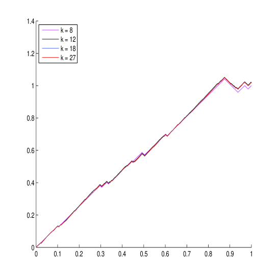
Figure 1. $B_{k}$ for $k=8,\ 12,\ 18,\ 27$ in the case $b=2$ and $H=0.95$: Fast strong convergence.

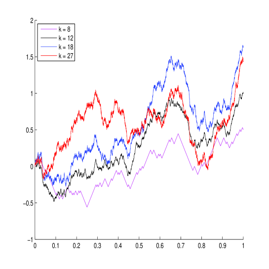
Figure 3. $B_{k}/\sigma\sqrt{k}$ for $k=8,\ 12,\ 18,\ 27$ in the case $b=2$ and $H=0.5$: Convergence in distribution to the Wierner Brownian motion.

When $H\in(1/2,1)$, the martingale $(B_{n})_{n\geq 1}$ indeed converges as expected as $n$ tends to $\infty$ (Theorem 1.1). This is illustrated in Figures 1 and 2. The pointwise Hölder exponent of the almost sure limit $B$ is equal to $H$ everywhere, and the Hausdorff dimension of the graph of $B$ is $2-H$. Moreover, the process $B$ possesses scaling invariance properties relative to the dyadic grid, with $H$ playing the role of a Hurst exponent, as can be seen by letting $n$ tend to $\infty$ in (1.3). Furthermore, the normalized process $B/\sqrt{\mathbb{E}(B(1)^{2})}$ converges in law to the standard Brownian motion as $H\searrow 1/2$ (Theorem 1.2). Thus, $B$ shares a lot of properties with fBm of exponent $H$, though it has not stationary increments and it is not Gaussian (see Remark 1.1). When $H\in(-\infty,1/2]$, the martingale is not bounded in $L^{2}$ norm and it diverges. However, the normalized sequence $B_{n}/\sqrt{\mathbb{E}(B_{n}(1)^{2})}$ converges in law to the standard Brownian motion as $n$ tends to $\infty$ (Theorem 1.3). This is illutrated in Figures 3 and 4. When $H<1/2$ this result is a version of Donsker’s theorem, but for triangular arrays with unusual strong correlations. When $H=1/2$, the same strong correlations hold, but $B_{n}/\sqrt{\mathbb{E}(B_{n}(1)^{2})}$ corresponds to a correlated random walk normalized in the same unusual way as very different correlated random walks considered in [10] and weakly converging to Brownian motion as well (see the discussion in Remark 1.3).

Our results are stated and commented in the following theorems and remarks. Then we relate them with some works on laws that are stable under random weighted mean.

$\mathcal{C}([0,1])$ will denote the space of real-valued continuous functions over $[0,1]$ endowed with the uniform norm denoted by $\|\ \,\|_{\infty}$, and ${\rm Id}_{[0,1]}$ will denote the identity function over $[0,1]$. We refer to [13] for the definitions of Hausdorff and box dimensions of sets in $\mathbb{R}^{d}$ as well as [6] for the theory of the convergence of probability measures on metric spaces.

The case $H\in(1/2,1]$.

Theorem 1.1.

Let $H\in(1/2,1]$. The $\mathcal{C}([0,1])$-valued martingale $(B_{n})_{n\geq 1}$ converges almost surely and in $L^{q}$ norm for all $q\geq 1$ to a limit function of expectation ${\rm{Id}}_{[0,1]}$. Denote this limit by $B$ and for all $w\in T$ the limit of $B_{n}(w)$ by $B(w)$. With probability 1,

1. For all $p\geq 1$, $w\in\{0,1\}^{p}$ and $t\in I_{w}$

   (1.4) $$B(t)-B(t_{w})=\boldsymbol{\epsilon}(w)\,2^{-pH}B(w)\left(S_{w_{p}}^{-1}\circ\cdots\circ S_{w_{1}}^{-1}(t)\right);$$

2. $B$ is $\alpha$-Hölder continuous for all $\alpha\in(0,H)$, and it has everywhere a pointwise Hölder exponent equal to $H$, i.e for all $t\in[0,1]$

   $$\liminf_{\begin{subarray}{c}s\to t\\ s\neq t\end{subarray}}\frac{\log|B(s)-B(t)|}{\log|s-t|}=H;$$

3. The Hausdorff and box dimensions of the graph of $B$ are equal to $2-H$.

For $H\in(1/2,1)$ define $\sigma_{H}=(2-2^{2-2H})^{-1/2}=\sqrt{\mathbb{E}(B(1)^{2})}$ (this equality will be justified in the proof of the next result) and denote $B$ by $B_{H}$.

Theorem 1.2.

The family of continuous processes $\{B_{H}/\sigma_{H}\}_{H\in(1/2,1)}$ converges in law, as $H$ tends to $1/2$, to the restriction to $[0,1]$ of the standard Brownian motion.

Remark 1.1.

When $H=1$, the weights are positive and the construction coincides with the trivial positive cascade: with probability 1, $B_{n}(t)=t$ for all $t\in[0,1]$ and $n\geq 1$. When $H\in(1/2,1)$, the limit process $B-\text{Id}_{[0,1]}$ is not fractional Brownian motion. This can be seen on (1.4) since $\boldsymbol{\epsilon}(w)$ is not symmetric. Also, a computation shows that the third moment of the centered random variable $B(1)-1$ does not vanish, so the process is not Gaussian.

The case $H\in[-\infty,1/2]$.

For $H\in(-\infty,1/2]$, the sequence $(B_{n})_{n\geq 1}$ is not bounded in $L^{2}$ norm. To get a natural normalization making it bounded in $L^{2}$ norm let

$$\sigma=\begin{cases}\displaystyle\sqrt{1+(2^{2-2H}-2)^{-1}}&\mbox{if $H<1/2$}\\ \displaystyle 1/{\sqrt{2}}&\mbox{if $H=1/2$}\\ \end{cases}$$

and for $w\in T$ and $n\geq 1$ define

$$X_{n}(w)=\begin{cases}B_{n}(w)/\sigma 2^{n(1/2-H)}&\mbox{if $H<1/2$}\\ B_{n}(w)/\sigma\sqrt{n}&\mbox{if $H=1/2$}\\ \end{cases}$$

Also simply denote $X_{n}(\emptyset)$ by $X_{n}$. The process $X_{n}$ is equivalent to $B_{n}/\sqrt{\mathbb{E}(B_{n}(1)^{2})}$ as $n$ tends to $\infty$ (this fact will be justified in the proof of the next result). If we let $H$ tend to $-\infty$ in the definition of $\epsilon$ and $\sigma$, then $\epsilon$ becomes a symmetric random variable taking values in $\{-1,1\}$, $\sigma=1$, and the sequence $(X_{n})_{n\geq 1}$ has the natural extension to the case $H=-\infty$ given by $X_{n}(t)=\displaystyle\frac{1}{\sqrt{2^{n}}}\left[S_{[2^{n}t]}^{(n)}+(2^{n}t-[2^{n}t])\xi_{[2^{n}t]}^{(n)}\right]$ (see Remark 1.3).

Theorem 1.3.

For every $H\in[-\infty,1/2]$ the sequence of continuous processes $(X_{n})_{n\geq 1}$ converges in law, as $n$ tends to $\infty$, to the restriction to $[0,1]$ of the standard Brownian motion.

Remark 1.2.

When $H\in(-\infty,1/2)$, $\limsup_{n\rightarrow\infty}\|B_{n}\|_{\infty}{2^{-n(1/2-H)}}>0$ almost surely by Theorem 1.3. Thus the martingale $(B_{n})_{n\geq 1}$ diverges in $\mathcal{C}([0,1])$. The same property holds when $H=1/2$. Besides, Theorem 1.1 says that $(B_{n})_{n\geq 1}$ converges almost surely uniformly to a limit of expectation $\text{Id}_{[0,1]}$ when $H>1/2$. Consequently, the convergence properties of non-positive canonical cascades strongly depend on the random weight used to generate the process. This contrasts with the positive canonical cascades martingales, which always converge almost surely uniformly (either to a non-trivial limit with expectation $\text{Id}_{[0,1]}$, or to 0, see [24, 19]).

Remark 1.3.

When $H\in(-\infty,1/2]$, due to (1.2) we have

(1.5) $$X_{n}(t)=\begin{cases}\displaystyle\frac{1}{\sigma\sqrt{2^{n}}}\left[S_{[2^{n}t]}^{(n)}+(2^{n}t-[2^{n}t])\xi_{[2^{n}t]}^{(n)}\right]&\text{if }H<1/2\\ \displaystyle\frac{1}{\sigma\sqrt{n2^{n}}}\left[S_{[2^{n}t]}^{(n)}+(2^{n}t-[2^{n}t])\xi_{[2^{n}t]}^{(n)}\right]&\text{if }H=1/2\end{cases}.$$

When $H<1/2$, the form of $X_{n}$ is familiar from Donsker’s theorem (see [6]) and its extensions to triangular arrays of random variables that are weakly dependent (see [6, 8]). However, the correlations of the $X_{n}$ dyadic increments are closely related to the natural ultrametric distance on $T$ and it seems difficult to find a way to reduce the behavior of $(X_{n})_{n\geq 1}$ to that of random walks with weakly dependent increments. When $H=1/2$, the $X_{n}$ dyadic increments are correlated as well, and the normalization of the random walk is similar to the unusual one met in the proof of Theorem 2 in [10] (see also Lemma 5.1 of [28]) to obtain the weak convergence to Brownian motion of certain centered stationary Gaussian random walks.

If we denote $X_{n}(w)(1)$ by $Y_{n}(w)$, the relation (1.7) below yields

(1.6) $$Y_{n+1}=\begin{cases}\displaystyle\frac{\epsilon(0)}{\sqrt{2}}Y_{n}(0)+\frac{\epsilon(1)}{\sqrt{2}}Y_{n}(1)&\text{if }H<1/2\\ \displaystyle\sqrt{\frac{n}{n+1}}\Big{(}\frac{\epsilon(0)}{\sqrt{2}}Y_{n}(0)+\frac{\epsilon(1)}{\sqrt{2}}Y_{n}(1)\Big{)}&\text{if }H=1/2.\end{cases}$$

Consequently, assuming that $X_{n}$ converges in law, we can guess thanks to (1.6) that the weak limit of $Y_{n}$ must be the standard normal distribution. Actually, to identify this limit we exploit the recursive equations (1.6) as well as recursive equations satisfied by the moments of the standard normal distribution (see (3.1) in the proof of Lemma 3.1). A similar approach exploiting the functional equation (2.2) is used to prove Theorem 1.2.

Letting $H$ tend to $-\infty$ yields $\sigma=1$ and a random variable $\epsilon$ that takes the values $-1$ and $1$ with equal probability $1/2$ so that the random walk $S_{r}^{(n)}$ becomes symmetric. In this case, the convergence in law to Brownian motion of $X_{n}$ (defined as in (1.5) in the limit $H=-\infty$) follows from standard arguments, since $X_{n}$ conditioned with respect to $\mathcal{G}_{n-1}=\sigma\big{\{}\boldsymbol{\epsilon}(w):w\in\{0,1\}^{n-1}\big{\}}$ satisfies the Donsker’s theorem assumptions (given $\mathcal{G}_{n-1}$, the $\xi_{k}^{(n)}$s are symmetric, independent, and take values $-1$ and $1$).

If $H\in(1/2,1)$ and $\sigma$ is defined as $\sigma=\sqrt{\mathbb{E}(B(1)^{2})-1}$, the same kind of argument can be used to prove that $X_{n}=(B-B_{n})/\sigma 2^{n(1/2-H)}$ also converges in law to Brownian motion. Indeed, due to (1.4), conditionally on $\sigma\big{\{}\boldsymbol{\epsilon}(w):w\in\{0,1\}^{n}\big{\}}$, the increments of the process $2^{n/2}X_{n}$ over the dyadic intervals of generation $n$ are $2^{n}$ independent centered random variables distributed like $(B(1)-1)/\sigma$ or $-(B(1)-1)/\sigma$, namely the $\boldsymbol{\epsilon}(w)(B(w)(1)-1)/\sigma$, $w\in\{0,1\}^{n}$, whose standard deviation is equal to 1.

A link with laws that are stable under random weighted mean

For $n\geq 0$ and $w\in T$ we denote by $Z_{n}(w)$ the random variable $B_{n}(w)(1)$, with the convention $B_{0}(w)(1)=1$. We simply write $Z_{n}$ for $Z_{n}(\emptyset)$. By construction, for every $n\geq 1$

(1.7) $$Z_{n}=2^{-H}\epsilon(0)Z_{n-1}(0)+2^{-H}\epsilon(1)Z_{n-1}(1),$$

where the random variables $\epsilon(0)$, $\epsilon(1)$, $Z_{n-1}(0)$ and $Z_{n-1}(1)$ are mutually independent, $\epsilon(0)$ and $\epsilon(1)$ are copies of $\epsilon$, and $Z_{n-1}(0)$ and $Z_{n-1}(1)$ are copies of $Z_{n-1}$. Relation (1.7) is central in the sequel. When the martingale $(Z_{n})_{n\geq 1}$ does converge to a non trivial limit $Z$ (see Theorem 1.1), it follows from (1.7) that the probability distribution of $Z$ provides a new family of what has been called law stable by random weighted mean or fixed points of the smoothing transformation ([24, 9, 14]). Indeed, there exist two independent copies $Z(0)$ and $Z(1)$ of $Z$, and two independent and identically distributed random variables $W(0)$ and $W(1)$ — namely, $2^{-H}\epsilon(0)$ and $2^{-H}\epsilon(1)$ — such that $(W(0),W(1))$ is independent of $(Z(0),Z(1))$ and $Z$ satisfies the following equality in distribution ($\equiv$)

(1.8) $$Z\equiv W(0)Z(0)+W(1)Z(1).$$

When $(W(0),W(1))$ is positive, the non-trivial positive solutions of this equation are described in [24, 19, 9, 14]. A class of non-positive solutions of (1.8) with positive $(W(0),W(1))$ has been exhibited in [22]; it naturally includes classical symmetric stable laws of index $\alpha\in[1,2]$, which obey (1.8) when $W(0)=W(1)=2^{-H}$ with $H=1/\alpha\in[1/2,1]$. Actually, the classical symmetric stable law of index $\alpha=1/H\in[1,2]$ satisfies equation (1.8) under the form $Z\equiv 2^{-H}\eta(0)Z(0)+2^{-H}\eta(1)Z(1)$ as soon as $\eta(0)$ and $\eta(1)$ are independent, take values $-1$ and $1$, and are independent of $(Z(0),Z(1))$, whatever be the distributions of $\eta(0)$ and $\eta(1)$. Consequently, when $(\eta(0),\eta(1))=(\epsilon(0),\epsilon(1))$, Theorem 1.1 provides for each $H\in(1/2,1]$ another probability distribution obeying the same functional equation as the classical symmetric stable law of index $1/H$. It is worth noting that the statistically self-similar stochastic processes associated with these solutions have very different behaviors. In the first case, if $H=1/\alpha\in(1/2,1]$ the process is a symmetric stable Lévy process $L_{\alpha}$ of index $\alpha$ (see [5]), so the distributions of the increments have no finite moments of order larger than or equal to $\alpha$, and the sample path of $L_{\alpha}$ have a dense set of discontinuities and are multifractal [17]. In the second case, the process is the random function $B$ of Theorem 1.1, the distributions of the dyadic increments have a finite moment of order $p$ for all $p>0$, and the sample path of $B$ are continuous and monofractal.

Remark 1.4.

Both the construction and results extend to the case when the construction grid is $b$-adic with $b\geq 3$. Then $W=\epsilon b^{-H}$, where $\epsilon=1$ with probability $(1+b^{H-1})/2$ and $\epsilon=-1$ with probability $(1-b^{H-1})/2$. The same results hold after formal replacement of the basis 2 by the basis $b$. Also, $\sigma=\sqrt{1-1/b}$ if $H=1/2$, $\sigma=\sqrt{1+(b-1)/(b^{2-2H}-b)}$ if $H<1/2$, and $\sigma_{H}=\sqrt{b-1}/\sqrt{b-b^{2-2H}}$ if $H>1/2$.

Theorems 1.1, 1.3 and 1.2 are proved in Sections 2, 3 and 4 respectively.

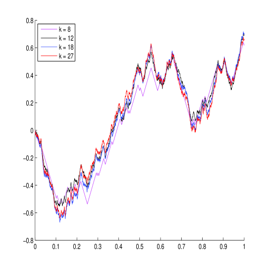
Figure 2. $B_{k}$ for $k=8,\ 12,\ 18,\ 27$ in the case $b=2$ and $H=0.7$. Strong convergence.

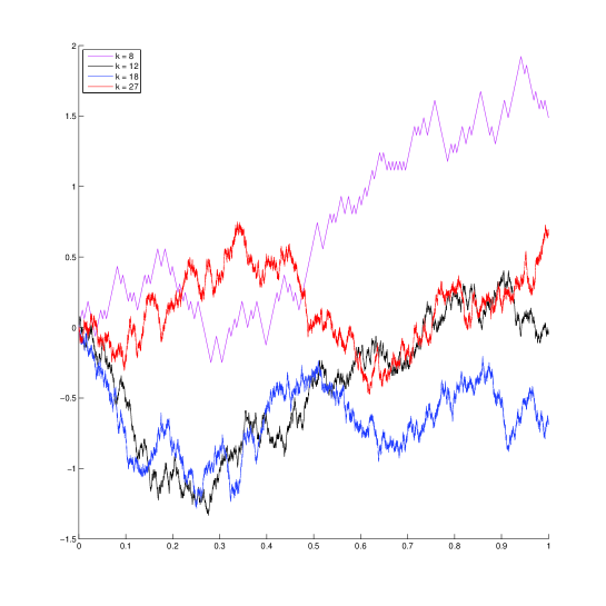
Figure 4. $B_{k}/\sigma b^{k(1/2-H)}$ for $k=8,\ 12,\ 18,\ 27$ in the case $b=2$ and $H=-2$: Convergence in distribution to the Wierner Brownian motion.

2. Proof of Theorem 1.1

Lemma 2.1.

The martingale $\big{(}Z_{n}=B_{n}(1)\big{)}_{n\geq 1}$ converges almost surely and in $L^{q}$ norm for all $q\geq 1$.

Proof.

For every integer $q\geq 1$, raising (1.7) to the power $q$ yields

(2.1) $$\mathbb{E}(Z_{n+1}^{q})=2^{1-qH}\mathbb{E}(\epsilon^{q})\mathbb{E}(Z_{n}^{q})+2^{-Hq}\sum_{k=1}^{q-1}\binom{q}{k}\mathbb{E}(\epsilon^{k})\mathbb{E}(\epsilon^{q-k})\mathbb{E}(Z_{n}^{k})\mathbb{E}(Z_{n}^{q-k}).$$

Moreover, since $H>1/2$ we have $0<2^{1-qH}\mathbb{E}(\epsilon^{q})<1$ for all integers $q\geq 2$ ($\mathbb{E}(\epsilon^{q})$ is equal to $2^{H-1}$ if $q$ is odd and 1 otherwise). Consequently, since $\mathbb{E}(Z_{n})=1$ for all $n\geq 1$, induction on $q\in\mathbb{N}^{*}$ using (2.1) shows that the sequence $\mathbb{E}(Z_{n}^{q})$ converges as $n$ tends to $\infty$ for every integer $q\geq 1$. This implies that the martingale $(Z_{n})_{n\geq 1}$ is bounded in $L^{q}$ norm for all $q\geq 1$, hence the result. ∎

Lemma 2.2.

Let $\alpha\in(0,H)$. With probability 1, there exists an integer $p_{0}\geq 1$ such that

$$\forall\ p\geq p_{0},\ \sup_{0\leq k\leq 2^{p}-1}\sup_{n\geq 1}\big{|}B_{n}\big{(}(k+1)2^{-p}\big{)}-B_{n}(k2^{-p})\big{|}\leq 2^{-p\alpha}.$$

Proof.

For every $p\geq 1$ and $0\leq k\leq 2^{p}-1$, by construction the sequence
$\left(\Delta B_{n}(p,k)=B_{n}\big{(}(k+1)2^{-p}\big{)}-B_{n}(k2^{-p})\right)_{n\geq 1}$ is a martingale, so Doob’s inequality yields for every $q>1$ a constant $C_{q}>0$ such that

$$\mathbb{E}\left(\sup_{n\geq 1}\big{|}\Delta B_{n}(p,k)\big{|}^{q}\right)\leq C_{q}\sup_{n\geq 1}\mathbb{E}\left(\big{|}\Delta B_{n}(p,k)\big{|}^{q}\right).$$

On the one hand — always by construction — if $n\leq p$, then $\mathbb{E}\left(\big{|}\Delta B_{n}(p,k)\big{|}^{q}\right)=2^{-qn(H-1)}2^{-qp}\leq 2^{-qpH}$ . On the other hand, (1.3) and Lemma 2.1 together yield a constant $C^{\prime}_{q}\geq 1$ such that $\mathbb{E}\left(\big{|}\Delta B_{n}(p,k)\big{|}^{q}\right)\leq C^{\prime}_{q}2^{-qpH}$ if $n>p$. Consequently, for all $p\geq 1$,

$$\mathbb{E}\left(\sup_{n\geq 1}\big{|}\Delta B_{n}(p,k)\big{|}^{q}\right)\leq C_{q}C^{\prime}_{q}2^{-qpH}.$$

For $q>(H-\alpha)^{-1}$, the previous inequality implies

$$\sum_{p\geq 1}\mathbb{P}\left(\exists\ 0\leq k<2^{p}:\sup_{n\geq 1}\big{|}\Delta B_{n}(p,k)\big{|}>2^{-p\alpha}\right)<\infty.$$

We conclude thanks to the Borel-Cantelli lemma. ∎

For $w\in T$ we define $Z(w)=\lim_{n\to\infty}Z_{n}(w)$, and we denote $Z$ by $Z(\emptyset)$.

Lemma 2.3.

Let $\varphi$ stand for the characteristic function of $Z$. There exists $\rho\in(0,1)$ such that $\varphi(t)=O\big{(}\rho^{|t|^{1/H}}\big{)}\ \ (|t|\to\infty)$. Consequently, the probability distribution of $Z$ possesses an infinitely differentiable bounded density, and $\mathbb{E}(|Z|^{-\gamma})<\infty$ for all $\gamma\in(0,1)$.

Proof.

The case $H=1$ is obvious. Suppose that $H\in(1/2,1)$. The probability distribution of $Z$ cannot be a Dirac mass, because $\mathbb{E}(Z)=1$ and

(2.2) $$Z=2^{-H}\epsilon(0)Z(0)+2^{-H}\epsilon(1)Z(1),$$

with the same independence and equidistribution properties as in (1.7). So there exists $\alpha>0$ and $\gamma<1$ such that $\sup_{t,|t|\in[\alpha,2^{H}\alpha]}|\varphi(t)|\leq\gamma$. Now, using the fact that

$$\varphi(t)=\left[p_{H}^{+}\varphi\big{(}2^{-H}t\big{)}+p_{H}^{-}\varphi\big{(}-2^{-H}t\big{)}\right]^{2},$$

we obtain by induction that $\displaystyle\sup_{t,\ |t|\in[2^{kH}\alpha,2^{(k+1)H]}\alpha]}|\varphi(t)|\leq\gamma^{2^{k}}\quad(\forall\ k\geq 0)$. Since $|t|^{1/H}\leq 2\alpha^{1/H}2^{k}$ for $|t|\in[2^{kH}\alpha,2^{(k+1)H}\alpha]$, the conclusion follows with $\rho=\gamma^{1/2\alpha^{1/H}}$.

The rate of decay of $\varphi$ at $\infty$ yields the conclusion regarding the probability distribution of $Z$ and the moments of $|Z|^{-1}$. ∎

Proof of Theorem 1.1: the convergence properties of $(B_{n})_{n\geq 1}$ and the global Hölder continuity of the limit process.

Let $\alpha\in(0,H)$. It follows from Lemma 2.2 that with probability 1, there exists $\delta>0$ and $C>0$ such that for all $(t,s)\in[0,1]^{2}$ such that $|t-s|\leq\delta$ we have $\sup_{n\geq 1}|B_{n}(t)-B_{n}(s)|\leq C|t-s|^{\alpha}$ (see for instance the proof of the Kolmogorov-Centsov theorem in [20]). Since the sequence $(B_{n})_{n\geq 1}$ converges almost surely on the set of dyadic numbers of $[0,1]$ which is dense in $[0,1]$, this implies that, with probability 1, $(B_{n})_{n\geq 1}$ converges uniformly to a limit $B$ which is $\alpha$-Hölder continuous. To see that the convergence holds in $L^{q}$ norm for all $q\geq 1$, it is enough to show that the sequence $\big{(}\mathbb{E}(\sup_{1\leq p\leq n}\|B_{p}\|_{\infty}^{q})\big{)}_{n\geq 1}$ is bounded for all integer $q\geq 2$. We show that it is true for $q=2$ and leave the reader verify by induction that it is true for $q\geq 2$. For $n\geq 1$, define

$$\widetilde{Z}_{n}=\sup_{1\leq p\leq n}\|B_{p}\|_{\infty},\mbox{ and }\widetilde{Z}_{n}(k)=\sup_{1\leq p\leq n}\|B_{p}(k)\|_{\infty},\ k\in\{0,1\}.$$

Due to (1.3) we have for $n\geq 2$

$$\widetilde{Z}_{n}\leq\max\Big{(}2^{-H}\widetilde{Z}_{n-1}(0),2^{-H}\widetilde{Z}_{n-1}(1)+\sup_{1\leq p\leq n}|B_{p}(1/2)|\Big{)}.$$

Thus, if we denote $\sup_{1\leq p\leq n}|B_{p}(1/2)|$ by $M_{n}$ we have

$$\mathbb{E}(\widetilde{Z}_{n}^{2})\!\!\! \leq \!\!\!\mathbb{E}\left(2^{-2H}\widetilde{Z}_{n-1}(0)^{2}+2^{-2H}\widetilde{Z}_{n-1}(1)^{2}+2\widetilde{Z}_{n-1}(1)M_{n}+M_{n}^{2}\right)$$

$$\leq \!\!\!2^{1-2H}\mathbb{E}(\widetilde{Z}_{n-1}^{2})+2\mathbb{E}(\widetilde{Z}_{n-1}^{2})^{1/2}\left\|M_{n}\right\|_{2}+\|M_{n}\|_{2}^{2}.$$

Lemma 2.1 shows that $(B_{p}(1/2))_{p\geq 1}$ is a martingale bounded in $L^{2}$ norm, so $(\left\|M_{n}\right\|_{2})_{n\geq 1}$ is bounded. Consequently, there exists $C>0$ such that

(2.3) $$\forall\ n\geq 1,\ \mathbb{E}(\widetilde{Z}_{n}^{2})\leq f\big{(}\mathbb{E}(\widetilde{Z}_{n-1}^{2})\big{)},\ \mbox{with }f(x)=2^{1-2H}x+C\sqrt{x}+C.$$

Since $2^{1-2H}<1$, there exists $x_{0}>0$ such that $f(x)<x$ for all $x>x_{0}$ . This fact together with (2.3) yields $\mathbb{E}(\widetilde{Z}_{n}^{2})\leq\max\left(x_{0},f\big{(}\mathbb{E}(\widetilde{Z}_{1}^{2})\big{)}\right)$ for all $n\geq 2$.

Proof of Theorem 1.1: the properties 1., 2. and 3.

1. This is an immediate consequence of (1.3).

2. The global Hölder regularity property has already been established. To obtain the pointwise Hölder exponent we use an approach similar to that used for the Brownian motion in [11] (see also [20]).

Fix $\varepsilon>0$ and let $\mathcal{O}$ be the set of points $\omega\in\Omega$ such that $B_{n}$ converges uniforlmy as $n\to\infty$ and the limit $B$ possesses points at which the pointwise Hölder exponent is at least $H+\varepsilon$. We show that $\mathcal{O}$ is included in a set of null probability.

We fix an integer $K>4/\varepsilon$ and denote by $n_{K}$ the smallest integer $n$ such that $K2^{-n}\leq 1$. For $t\in[0,1]$ and $n\geq n_{K}$ , consider $S^{K}_{n}(t)$ a subset of $[0,1]$ consisting of $K+1$ consecutive dyadic numbers of generation $n$ such that $t\in[\min\,S^{K}_{n}(t),\max\,S^{K}_{n}(t)]$. Also denote by $\boldsymbol{S}^{K}_{n}(t)$ the set of $K$ consecutive dyadic intervals delimited by the elements of $S^{K}_{n}(t)$. If the pointwise Hölder exponent at $t$ is larger than or equal to $H+\varepsilon$ then for $n$ large enough we have necessarily $\sup_{s\in S^{K}_{n}(t)}|B(s)-B(t)|\leq(K2^{-n})^{H+\varepsilon/2}$, so that $\sup_{I\in\boldsymbol{S}^{K}_{n}(t)}|\Delta B(I)|\leq 2(K2^{-n})^{H+\varepsilon/2}$, where $\Delta B(I)$ stands for the increment of $B$ over $I$.

Now let $\boldsymbol{S}^{K}_{n}$ be the set consisting of all $K$-uple of consecutive dyadic intervals of generation $n$, and if $S\in\boldsymbol{S}^{K}_{n}$, denote the event $\big{\{}\sup_{I\in S}|\Delta B(I)|\leq 2(K2^{-n})^{H+\varepsilon/2}\big{\}}$ by $E_{S}$. The previous lines show that

$$\mathcal{O}\subset\mathcal{O}^{\prime}=\bigcap_{n\geq n_{K}}\bigcup_{p\geq n}\bigcup_{S\in\boldsymbol{S}^{K}_{p}}E_{S}.$$

By construction, if $S\in\boldsymbol{S}^{K}_{p}$, $\big{(}|\Delta B(I)|\big{)}_{I\in S}$ is equal to $(2^{-pH}|Y_{I}|)_{I\in S}$, where the $K$ random variables $Y_{I}$ are mutually independent and identically distributed with $B(1)$. Consequently, $\mathbb{P}(E_{S})$ depends only on $K$ and $p$ and

$$\mathbb{P}(E_{S}) \leq \left[\mathbb{P}(|B(1)|\leq 2K^{H}(K2^{-p})^{\varepsilon/2})\right]^{K}$$

$$\leq (2K^{H})^{K/2}K^{K\varepsilon/4}2^{-pK\varepsilon/4}\left[\mathbb{E}(|B(1)|^{-1/2})\right]^{K},$$

where $\mathbb{E}(|B(1)|^{-1/2})<\infty$ due to Lemma 2.3. Since the cardinality of $\boldsymbol{S}^{K}_{p}$ is less than $2^{p}$, this yields $\mathbb{P}\big{(}\bigcup_{S\in\boldsymbol{S}^{K}_{p}}E_{S}\big{)}=O(2^{p}2^{-pK\varepsilon/4})$. Our choice for $K$ implies that the series $\sum_{p\geq n_{K}}\mathbb{P}\big{(}\bigcup_{S\in\boldsymbol{S}^{K}_{p}}E_{S}\big{)}$ converges, hence $\mathbb{P}(\mathcal{O}^{\prime})=0$.

3. Let us introduce additional notations. If $w\in\Sigma^{*}$ and $J=I_{w}$ then we define $\boldsymbol{\epsilon}(J):=\boldsymbol{\epsilon}(w)=\prod_{k=1}^{|w|}\epsilon(w_{1}\cdots w_{k})$. We denote by $\Gamma$ the graph $\left\{\big{(}t,B(t)\big{)}:t\in[0,1]\right\}$ of $B$. We recall that the Hausdorff dimension of a subset of $\mathbb{R}^{2}$ is always smaller than of equal to its box dimension.

At first, since $B$ is $\alpha$-Hölder continuous for all $\alpha<H$, $2-H$ is an upper bound for the box dimension of $\Gamma$ (see [13] Ch. 11).

To find the sharp lower bound $2-H$ for the Hausdorff dimension of $\Gamma$ we show that, with probability 1, the measure on this graph obtained as the image of the Lebesgue measure restricted to $[0,1]$ by the mapping $t\mapsto\big{(}t,B(t)\big{)}$ has a finite energy with respect to the Riesz Kernel $u\in\mathbb{R}^{2}\setminus\{0\}\mapsto\|u\|^{-\gamma}$ for all $\gamma<2-H$ (see [13] Ch. 4.3 and 11 for details about this kind of approach). This property holds if we show that for all $\gamma<2-H$ we have

$$\int_{[0,1]^{2}}\mathbb{E}\left(\big{(}|t-s|^{2}+|B(t)-B(s)|^{2}\big{)}^{-\gamma/2}\right)\ \text{d}t\text{d}s<\infty.$$

If $I$ is a closed subinterval of $[0,1]$, we denote by $\mathcal{G}(I)$ the set of closed dyadic intervals of maximal length included in $I$, and then $m_{I}=\min\bigcup_{J\in\mathcal{G}(I)}J$ and $M_{I}=\max\bigcup_{J\in\mathcal{G}(I)}J$.

Let $0<s<t<1$ be two non dyadic numbers. We define two sequences $(s_{p})_{p\geq 0}$ and $(t_{p})_{p\geq 0}$ as follows. Let $s_{0}=m_{[s,t]}$ and $t_{0}=M_{[s,t]}$. Then let define inductively $(s_{p})_{p\geq 1}$ and $(t_{p})_{p\geq 1}$ as follows: $s_{p}=m_{[s,s_{p-1}]}$ and $t_{p}=M_{[t_{p-1},t]}$. Let us denote by $\mathcal{C}$ the collection of intervals consisting of $[s_{0},t_{0}]$ and all the intervals $[s_{p},s_{p-1}]$ and $[t_{p-1},t_{p}]$, $p\geq 1$. Every interval $I\in\mathcal{C}$ is the union of at most two intervals of the same generation $n_{I}$, the elements of $\mathcal{G}(I)$, and

$$\Delta B(I)=\sum_{J\in\mathcal{G}(I)}\Delta B(J)=\sum_{J\in\mathcal{G}(I)}\boldsymbol{\epsilon}(J)2^{-n_{I}H}Y_{J},$$

where $\Delta B(J)$ and $Y(J)$ have been introduced in the discussion regarding the pointwise exponents. By construction, we have $\min_{I\in\mathcal{C}}n_{I}=n_{[s_{0},t_{0}]}$ and $(t-s)/3\leq 2^{-n_{[s_{0},t_{0}]}}\leq(t-s)$. Also, all the random variables $Y_{J}$ are mutually independent and independent of $\mathcal{T}_{\mathcal{C}}=\sigma(\boldsymbol{\epsilon}(J):J\in\mathcal{G}(I),\ I\in\mathcal{C})$. Now, we write

$$B(t)-B(s)=2^{-n_{[s_{0},t_{0}]}H}\Big{(}\sum_{J\in\mathcal{G}([s_{0},t_{0}])}\boldsymbol{\epsilon}(J)Y_{J}+Z(s,s_{0})+Z(t_{0},t)\Big{)},$$

where

$$\begin{cases}\displaystyle Z(s,s_{0})=\lim_{p\to\infty}\sum_{0\leq k\leq p}2^{(n_{[s_{0},t_{0}]}-n_{[s_{k+1},s_{k}]})H}\sum_{J\in\mathcal{G}([s_{k+1},s_{k}])}\boldsymbol{\epsilon}(J)Y_{J}\\ \displaystyle Z(t_{0},t)=\lim_{p\to\infty}\sum_{0\leq k\leq p}2^{(n_{[s_{0},t_{0}]}-n_{[t_{k},t_{k+1}]})H}\sum_{J\in\mathcal{G}([t_{k},t_{k+1}])}\boldsymbol{\epsilon}(J)Y_{J}.\end{cases}$$

Let $\mathcal{Z}(t,s)=\sum_{J\in\mathcal{G}([s_{0},t_{0}])}\boldsymbol{\epsilon}(J)Y_{J}+Z(s,s_{0})+Z(t_{0},t)$ and fix $J_{0}\in\mathcal{G}([s_{0},t_{0}])$. Conditionally on $\mathcal{T}_{\mathcal{C}}$, $\mathcal{Z}(t,s)$ is the sum of $\pm Y(J_{0})$ plus a random variable $U$ independent of $Y(J_{0})$. Consequently, the probability distribution of $\mathcal{Z}(t,s)$ conditionally on $\mathcal{T}_{\mathcal{C}}$ possesses a density $f_{t,s}$ and $\|\widehat{f_{t,s}}\|_{L^{1}}\leq\|\varphi\|_{L^{1}}$, where $\varphi$ is the characteristic function of $Y(J_{0})$ studied in Lemma 2.3.

Thus, for $\gamma<2-H$ we have

$$\mathbb{E}\left(\big{(}|t-s|^{2}+|B(t)-B(s)|^{2}\big{)}^{-\gamma/2}|\mathcal{T}_{\mathcal{C}}\right) =\int_{\mathbb{R}}\frac{f_{t,s}(u)}{\big{(}|t-s|^{2}+2^{-2n_{[s_{0},t_{0}]}H}u^{2}\big{)}^{\gamma/2}}\,\text{d}u$$

$$\leq\int_{\mathbb{R}}\frac{f_{t,s}(u)}{\big{(}|t-s|^{2}+3^{-2H}(t-s)^{2H}u^{2}\big{)}^{\gamma/2}}\,\text{d}u$$

$$=|t-s|^{1-H-\gamma}\int_{\mathbb{R}}\frac{f_{t,s}(|t-s|^{1-H}v)}{\big{(}1+3^{-2H}v^{2}\big{)}^{\gamma/2}}\,\text{d}v.$$

The function $f_{t,s}$ is bounded independently of $t,\ s$ and $\mathcal{T}_{\mathcal{C}}$ since it is bounded by $\|\widehat{f_{t,s}}\|_{L^{1}}$ and we just saw that this number is bounded by $\|\varphi\|_{L^{1}}$. Thus,

$$\mathbb{E}\left(\big{(}|t-s|^{2}+|B(t)-B(s)|^{2}\big{)}^{-\gamma/2}\right)\leq\|\varphi\|_{L^{1}}|t-s|^{1-H-\gamma}\int_{\mathbb{R}}\frac{\text{d}v}{\big{(}1+3^{-2H}v^{2}\big{)}^{\gamma/2}}.$$

This yields the conclusion. Notice that the fact that the distribution of the increment of $B$ over $[0,1]$, namely $Z$, has a density plays a crucial role in this proof, as the same kind of property is a powerful tool in finding a lower bound for the Hausdorff dimension of the graphs of fractional Brownian motions, symmetric Lévy processes of index $\alpha\in(1,2)$ and certain Weierstrass functions with random phases (see [13, 16]).

3. Proof of Theorem 1.3

The case $H=-\infty$ has been discussed in Remark 1.3. We fix $H\in(-\infty,1/2]$.

Lemma 3.1.

The sequence $(X_{n}(1))_{n\geq 1}$ converges in law to the standard normal distribution as $n$ tends to $\infty$.

Proof.

Let $u_{0}=\mathbb{E}(Z_{0}^{2})=1$. By definition, we have $u_{0}=1$. Let $\ell$ be the solution of $\ell=2^{1-2H}\ell+\frac{1}{2}$ when $H<1/2$, i.e. $\ell=(2-2^{2-2H})^{-1}$. Taking successively the square and the expectation in (1.7) yields $\displaystyle\mathbb{E}(Z_{n}^{2})=2^{1-2H}\mathbb{E}(Z_{n-1}^{2})+\frac{1}{2}$ for $n\geq 1$. Consequently, $\mathbb{E}(Z_{n}^{2})=\ell+2^{n(1-2H)}(u_{0}-\ell)$ if $H>1/2$ and $\mathbb{E}(Z_{n}^{2})=u_{0}+n/2$ if $H=1/2$. This yields $\mathbb{E}(Z_{n}^{2})\sim\frac{2^{2-2H}-1}{2^{2-2H}-2}2^{n(1-2H)}=\sigma^{2}2^{n(1-2H)}$ if $H<1/2$ and $\mathbb{E}(Z_{n}^{2})\sim n/2=\sigma^{2}n$ if $H=1/2$. This is why we consider the normalized processes $X_{n}$.

For $n\geq 1$ and $q\geq 1$ let $M_{n}^{(q)}=\mathbb{E}(X_{n}(1)^{q})$. We are going to prove by induction and by using (1.7) that

1. for every $p\geq 0$ one has the property $(\mathcal{P}_{2p})$: $M^{(2p)}=\lim_{n\to\infty}M_{n}^{(2p)}$ exists; moreover $M^{(2)}=1$;

2. for every $p\geq 0$ one has the property $(\mathcal{P}_{2p+1})$: $\lim_{n\to\infty}M_{n}^{(2p+1)}=0$;

3. the sequence $(M^{(2p)})_{p\geq 1}$ obeys the following induction relation valid for $p\geq 2$:

   (3.1) $$M^{(2p)}=\big{(}2^{p}-2\big{)}^{-1}\sum_{k=1}^{p-1}\binom{2p}{2k}M^{(2k)}M^{(2p-2k)}.$$

Suppose that these properties have been established. Then, 1. insures that the probability distributions of the $X_{n}(1)$ form a tight sequence. Moreover, it is easy to verify that a $\mathcal{N}(0,1)$ random variable $N$ has the property that its moments of even orders satisfy the same relation as the numbers $M_{2p}$, $p\geq 1$, defined by $M_{2}=1$ and the induction relation 3. To see this, write $N$ as the sum of two independent $\mathcal{N}(0,2^{-1/2})$ random variables. Consequently, since the law $\mathcal{N}(0,1)$ is characterized by its moments, 1., 2. and 3. imply that $X_{n}(1)$ converges in law to $\mathcal{N}(0,1)$.

Now we prove 1., 2., and 3.. By construction, we have $M_{n}^{(1)}\sim 1/(\mathbb{E}(Z_{n}^{2}))^{1/2}$ hence $\lim_{n\to\infty}M_{n}^{(1)}=0$, as well as $\lim_{n\to\infty}M_{n}^{(2)}=1$. Consequently, $(\mathcal{P}_{1})$ and $(\mathcal{P}_{2})$ hold.

Let $q$ be an integer $\geq 3$. Raising (1.6) to the power $q$ yields

(3.2) $$M_{n+1}^{(q)}=\displaystyle r_{n}^{q}\left(2^{1-q/2}\mathbb{E}(\epsilon^{q})\mathbb{E}(Z_{n}^{q})+2^{-q/2}S(q,n)\right),$$

where $r_{n}=\displaystyle\sqrt{\frac{n}{n+1}}$ if $H=1/2$ and $r_{n}=1$ otherwise, and

$$S(q,n)=\sum_{k=1}^{q-1}\binom{q}{k}\mathbb{E}(\epsilon^{k})\mathbb{E}(\epsilon^{q-k})M_{n}^{(k)}M_{n}^{(q-k)}.$$

Since $\mathbb{E}(\epsilon_{0}^{q})=2^{H-1}$ or $1$ according to $q$ is odd or even, (3.2) yields

(3.3) $$M_{n+1}^{(q)}=\begin{cases}\displaystyle r_{n}^{q}\left(2^{H-q/2}M_{n}^{(q)}+2^{-q/2}S(q,n)\right)&\mbox{if $q$ is odd},\\ \displaystyle r_{n}^{q}\left(2^{1-q/2}M_{n}^{(q)}+2^{-q/2}S(q,n)\right)&\mbox{if $q$ is even}\end{cases}.$$

Let us show by induction that $\big{(}(\mathcal{P}_{2p-1}),(\mathcal{P}_{2p})\big{)}$ holds for $p\geq 1$, as well as (3.1).

We have already shown that $\big{(}(\mathcal{P}_{1}),(\mathcal{P}_{2})\big{)}$ holds. Suppose that $\big{(}(\mathcal{P}_{2k-1}),(\mathcal{P}_{2k})\big{)}$ holds for $1\leq k\leq p-1$, with $p\geq 2$. In particular, $M_{n}^{(k)}$ tends to 0 as $n$ tend to $\infty$ if $k$ is an odd integer belonging to $[1,2p-3]$. Consequently, $S(2p-1,n)$ tends to 0 as $n$ tends to $\infty$; indeed, for each integer $k$ between $1$ and $2p-1$, either $k$ or $2p-1-k$ is an odd number. The sequence $(r_{n})_{n\geq 1}$ being bounded, it follows from this property and (3.3) that $\displaystyle M_{n+1}^{(2p-1)}=r_{n}^{2p-1}2^{H+1/2-p}M_{n}^{(2p-1)}+o(1)$ as $n\to\infty$. Since $r_{n}^{2p-1}2^{H+1/2-p}\leq 2^{1-p}<1$, this yields $\lim_{n\to\infty}M_{n}^{(2p-1)}=0$, that is to say $(\mathcal{P}_{2p-1})$.

Also, our induction’s assumption implies that in the right hand side of $M_{n+1}^{(2p)}$, the term $S(2p,n)$ tends to $L=\sum_{k=1}^{p-1}\binom{2p}{2k}M^{(2k)}M^{(2p-2k)}$ as $n$ tends to $\infty$. Define $L^{\prime}=(2^{p}-2)^{-1}L$. By using (3.3) we deduce from the previous lines that

$$M_{n+1}^{(2p)}=\begin{cases}r_{n}^{2p}2^{1-p}M_{n}^{(2p)}+2^{-p}L+o(1)&\text{if }H=1/2\\ 2^{1-p}M_{n}^{(2p)}+2^{-p}L+o(1)&\text{if }H<1/2\end{cases}.$$

Since $r_{n}\to 1$ as $n\to\infty$ when $H=1/2$ and $L^{\prime}=2^{1-p}L^{\prime}+2^{-p}L$ we obtain

$$M_{n+1}^{(2p)}-L^{\prime}=\begin{cases}r_{n}^{2p}2^{1-p}(M_{n}^{(2p)}-L^{\prime})+o(1)&\text{if }H=1/2\\ 2^{1-p}(M_{n}^{(2p)}-L^{\prime})+o(1)&\text{if }H<1/2\end{cases}.$$

This yields both $(\mathcal{P}_{2p})$ and (3.1) since $r_{n}\leq 1$ and $2^{1-p}<1$. ∎

Lemma 3.2.

The laws of the random continuous functions $X_{n}$, $n\geq 1$, form a tight family in the set of probability measures on $\mathcal{C}([0,1])$.

Proof.

By Theorem 7.3 of [6], since $X_{n}(0)=0$ almost surely for all $n\geq 1$, it is enough to show that for each positive $\varepsilon$

(3.4) $$\lim_{\delta\to 0}\limsup_{n\to\infty}\mathbb{P}\big{(}\omega(X_{n},\delta)\geq\varepsilon\big{)}=0,$$

where $\omega(X_{n},\cdot)$ stands for the modulus of continuity of $X_{n}$.

We leave the reader to check the following simple properties for $p,n\geq 1$ and $w\in\{0,1\}^{p}$: If $n>p$ then

(3.5) $$X_{n}(t_{w}+2^{-p})-X_{n}(t_{w})=\boldsymbol{\epsilon}(w)2^{-p/2}\cdot\begin{cases}X_{n-p}(w)(1)&\mbox{if $H<1/2$}\\ \displaystyle\sqrt{\frac{n-p}{n}}X_{n-p}(w)(1)&\mbox{if $H=1/2$}\end{cases}$$

and if $1\leq n\leq p$ then

(3.6) $$|X_{n}(t_{w}+2^{-p})-X_{n}(t_{w})|\leq\begin{cases}\displaystyle 2^{-p/2}/\sigma&\mbox{if $H<1/2$}\\ \displaystyle 2^{-p/2}/\sigma\sqrt{n}&\mbox{if $H=1/2$}\\ \end{cases}.$$

Moreover, the proof of Lemma 3.1 shows that $\sup_{n\geq 1}\mathbb{E}(X_{n}(1)^{2K})<\infty$ for every integer $K\geq 1$. Consequently, it follows from (3.5) and (3.6) that there exists a family $\{V_{n,p,k}\}_{n,p\geq 1,0\leq k\leq 2^{p}-1}$ of positive random variables such that

$$\left|X_{n}\big{(}(k+1)2^{-p}\big{)}-X_{n}\big{(}k2^{-p}\big{)}\right|\leq 2^{-p/2}V_{n,p,k},$$

and for any integer $K\geq 1$, $C_{K}=\sup_{\begin{subarray}{c}n,p\geq 1\\ 0\leq k\leq 2^{p}-1\end{subarray}}\mathbb{E}(V_{n,p,k}^{2K})<\infty$. The end of the proof is then standard.

Fix $\alpha\in(0,1/2)$ and $K$ a positive integer such that $2K(1/2-\alpha)>1$. Define $\rho_{p}=C_{K}2^{p(1+2K(\alpha-1/2))}$ and $R_{p}=\sum_{j\geq p}\rho_{j}$ for $p\geq 1$. For all $n,p\geq 1$, our control of the moments of the dyadic increments of $X_{n}$ yields, using Markov inequalities, $\mathbb{P}\Big{(}\bigcup_{0\leq k<2^{p}}\ \left\{\left|X_{n}\big{(}(k+1)2^{-p}\big{)}-X_{n}\big{(}k2^{-p}\big{)}\right|>2^{-p\alpha}\right\}\Big{)}\leq\rho_{p}$.

Thus, $\inf_{n\geq 1}\mathbb{P}(E^{n}_{p})\geq 1-R_{p}$ for all $p\geq 1$, where

$$E^{n}_{p}=\left\{\forall\ j\geq p,\ \forall\ 0\leq k<2^{-j},\ \left|X_{n}\big{(}(k+1)2^{-j}\big{)}-X_{n}\big{(}k2^{-j}\big{)}\right|\leq 2^{-j\alpha}\right\}.$$

Also, on $E^{n}_{p}$ we have $\displaystyle\omega\big{(}X_{n},2^{-p}\big{)}\leq 2^{1-p\alpha}/(1-2^{-\alpha}).$ This yields

$$\inf_{n\geq 1}\mathbb{P}\left(\omega\big{(}X_{n},2^{-p}\big{)}\leq 2^{1-p\alpha}/(1-2^{-\alpha})\right)\geq\inf_{n\geq 1}\mathbb{P}(E^{n}_{p})\geq 1-R_{p}.$$

Since $\lim_{p\to\infty}R_{p}=0$, the previous inequality gives (3.4). ∎

Proof of Theorem 1.3. Since for all $p\geq 1$ the random sequences $(X_{n}(w))_{n\geq 1}$, $w\in\{0,1\}^{p}$, are mutually independent, it follows from (3.5) and Lemma 3.1 that for all $p\geq 1$, the sequence of vectors $V_{n}(p)=\big{(}X_{p+n}(t_{w}+2^{-p})-X_{p+n}(t_{w})\big{)}_{w\in\{0,1\}^{p}}$ converges in law, as $n$ tends to $\infty$, to the distribution of the increments of the standard Brownian motion on the dyadic subintervals of $[0,1]$ of generation $p$. This is seen by taking the limit as $n$ tends to $\infty$ of the characteristic function of $V_{n}(p)$ conditionally on $\sigma\big{(}\boldsymbol{\epsilon}(w),\ w\in\{0,1\}^{p}\big{)}$ and then by using the fact that $\boldsymbol{\epsilon}(w)^{2}=1$. Consequently, the only possible weak limit of a subsequence of $(X_{n})_{n\geq 1}$ is the standard Brownian motion. Then Lemma 3.2 yields the desired conclusion.

4. Proof of Theorem 1.2

Theorem 1.2 follows from the next proposition. For $H\in(1/2,1)$ and $w\in T$ we denote $B_{H}(w)/\sigma_{H}$ by $\widetilde{B}_{H}(w)$ ($\widetilde{B}_{H}(\emptyset)=B_{H}/\sigma_{H}$ is denoted $\widetilde{B}_{H}$).

Proposition 4.1.

Let $(H_{m})_{m\geq 1}$ be a $(1/2,1)$-valued sequence converging to $1/2$ as $n\to\infty$.

1. The sequence $(\widetilde{B}_{H_{m}}(1))_{m\geq 1}$ converges in law to the standard normal distribution as $m$ tends to $\infty$.

2. The laws of the random continuous functions $\widetilde{B}_{H_{m}}$, $m\geq 1$, form a tight family in the set of probability measures on $\mathcal{C}([0,1])$.

3. For every $p\geq 1$, the sequence of vectors $\widetilde{V}_{m}(p)=\big{(}\widetilde{B}_{H_{m}}(t_{w}+2^{-p})-\widetilde{B}_{H_{m}}(t_{w})\big{)}_{w\in\{0,1\}^{p}}$ converges in law, as $m$ tends to $\infty$, to the distribution of the increments of the standard Brownian motion on the dyadic subintervals of $[0,1]$ of generation $p$.

Proof.

1. The proof is close to that of Lemma 3.1, but the differences deserve to be made explicit.

For every $q,m\geq 1$, let us denote $\mathbb{E}(\widetilde{B}_{H_{m}}(1)^{q})$ by $\widetilde{M}^{(q)}_{m}$. Since $H=H_{m}>1/2$ and by definition $\widetilde{B}_{H_{m}}(1)=\sqrt{2-2^{2-2H_{m}}}B(1)=\sqrt{2-2^{2-2H_{m}}}Z$, taking the limit in (2.1) as $n\to\infty$ thanks to Lemma 2.1 and using the fact that $\mathbb{E}(\epsilon_{0}^{q})=2^{H-1}$ or $1$ according to $q$ is odd or even, we obtain

(4.1) $$\widetilde{M}_{m}^{(q)}=\begin{cases}\displaystyle 2^{-(q-1)H_{m}}\widetilde{M}_{m}^{(q)}+2^{-qH_{m}}\widetilde{S}(q,m)&\mbox{if $q$ is odd},\\ \displaystyle 2^{1-qH_{m}}\widetilde{M}_{m}^{(q)}+2^{-qH_{m}}\widetilde{S}(q,m)&\mbox{if $q$ is even}\end{cases},$$

where $\displaystyle\widetilde{S}(q,m)=\sum_{k=1}^{q-1}\binom{q}{k}\mathbb{E}(\epsilon^{k})\mathbb{E}(\epsilon^{q-k})\widetilde{M}_{m}^{(k)}\widetilde{M}_{m}^{(q-k)}.$ Now we prove by induction that

1. for every $p\geq 0$ one has the property $(\mathcal{P}_{2p})$: $\widetilde{M}^{(2p)}=\lim_{m\to\infty}\widetilde{M}^{(2p)}_{m}$ exists. Moreover $\widetilde{M}^{(2)}=1$;

2. for every $p\geq 0$ one has the property $(\mathcal{P}_{2p+1})$: $\lim_{m\to\infty}\widetilde{M}^{(2p+1)}_{m}=0$;

3. the sequence $(\widetilde{M}^{(2p)})_{p\geq 1}$ obeys the same induction relation (3.1) as the sequence $(M^{(2p)})_{p\geq 1}$ defined in the proof of Lemma 3.1.

The conclusion is then the same as in the proof of Lemma 3.1.

To prove that $(\mathcal{P}_{1})$ and $(\mathcal{P}_{2})$ hold we first recall that $H$ being fixed, we have seen in the proof of Lemma 3.1 that $\displaystyle\mathbb{E}(Z_{n}^{2})=2^{1-2H}\mathbb{E}(Z_{n-1}^{2})+\frac{1}{2}$. For $H>1/2$ this yields $\mathbb{E}(Z^{2})=\lim_{n\to\infty}\mathbb{E}(Z_{n}^{2})=(2-2^{2-2H})^{-1}$. Consequently, $\mathbb{E}(\widetilde{B}_{H}(1))=\sqrt{2-2^{2-2H}}\mathbb{E}(B(1))=\sqrt{2-2^{2-2H}}$ tends to $0$ as $H\searrow 1/2$ and $\mathbb{E}(\widetilde{B}_{H}(1)^{2})=1$.

Suppose that $\big{(}(\mathcal{P}_{2k-1}),(\mathcal{P}_{2k})\big{)}$ holds for $1\leq k\leq p-1$, with $p\geq 2$. The same approach as in the proof of Lemma 3.1 implies that in (4.1), the term $2^{-(2p-1)H_{m}}\widetilde{S}(2p-1,m)$ in the right hand side of $\widetilde{M}_{m}^{(2p-1)}$ tends to 0 as $m$ tends to $\infty$. This implies $\displaystyle\widetilde{M}_{m}^{(2p-1)}=2^{-(2p-2)H_{m}}\widetilde{M}_{m}^{(2p-1)}+o(1)$ as $m\to\infty$. Since $2^{-(2p-2)H_{m}}\leq 2^{-(p-1)}<1$, this yields $\lim_{m\to\infty}M_{m}^{(2p-1)}=0$, that is to say $(\mathcal{P}_{2p-1})$. The induction’s assumption also implies that in the right hand side of $\widetilde{M}_{m}^{(2p)}$, the term $\widetilde{S}(2p,m)$ tends to $L=\sum_{k=1}^{p-1}\binom{2p}{2k}\widetilde{M}^{(2k)}\widetilde{M}^{(2p-2k)}$ as $m$ tends to $\infty$. Define $L^{\prime}=(2^{p}-2)^{-1}L$. By using (4.1) we deduce from the previous lines that $M_{m}^{(2p)}=2^{1-2pH_{m}}M_{m}^{(2p)}+2^{-p}L+o(1)$ as $m\to\infty$. As $2^{1-2pH_{m}}$ tends to $2^{1-p}$ as $m\to\infty$, the definition of $L^{\prime}$ implies $M_{m}^{(2p)}-L^{\prime}=2^{1-2pH_{m}}(M_{m}^{(2p)}-L^{\prime})+o(1)$ as $m\to\infty$. Since $2^{1-p}<1$ the last equality yields both $(\mathcal{P}_{2p})$ and (3.1) for $(\widetilde{M}^{(2p)})_{p\geq 1}$ instead of $(M^{(2p)})_{p\geq 1}$.

2. If $H\in(1/2,1)$, $p\geq 1$ and $w\in\{0,1\}^{p}$, due to Theorem 1.1.1 we have

(4.2) $$\widetilde{B}_{H}(t_{w}+2^{-p})-\widetilde{B}_{H}(t_{w})=\boldsymbol{\epsilon}(w)2^{-pH}\widetilde{B}_{H}(w)(1).$$

This implies $\left|\widetilde{B}_{H_{m}}(t_{w}+2^{-p})-\widetilde{B}_{H_{m}}(t_{w})\right|\leq 2^{-p/2}|\widetilde{B}_{H_{m}}(w)(1)|$. Moreover, the proof of 1. above shows that $C_{K}=\sup_{m\geq 1}\mathbb{E}(|\widetilde{B}_{H_{m}}(1)|^{2K})<\infty$ for every integer $K\geq 1$. We conclude as in the proof of Lemma 3.2.

3. Use (4.2) and the same arguments as in the proof of Theorem 1.3 as well as the fact that $2^{-pH_{m}}$ tends to $2^{-p/2}$ as $m\to\infty$. ∎

References

- [1] M. Arbeiter and N. Patzschke, Random self-similar multifractals, Math. Nachr., 181 (1996), 5–42.
- [2] J. Barral, Continuity of the multifractal spectrum of a statistically self-similar measure, J. Theoretic. Probab., 13 (2000), 1027–1060.
- [3] J. Barral, B.B. Mandelbrot, Random multiplicative multifractal measures. Proc. Symp. Pure Math., 72, Part 2, pp 3–90. AMS, Providence, RI (2004).
- [4] J. Barral, S. Seuret, The singularity spectrum of Lévy processes in multifractal time, Adv. Math., 214 (2007), 437–468.
- [5] J. Bertoin, Lévy processes, Cambridge University Press, 1996.
- [6] P. Billingsley, Convergence of Probability Measures, Wiley Series in Probability and Statistics. Second Edition, 1999.
- [7] P. Collet P, F. Koukiou, Large deviations for multiplicative chaos, Comm. Math. Phys. 147(1992), 329-342.
- [8] J. Dedecker, P. Doukhan, G. Lang, J. R. León R., S. Louhichi, C. Prieur. Weak dependence: with examples and applications. Lecture Notes in Statistics, 190. Springer, New York, 2007.
- [9] R. Durrett and T. Liggett, Fixed points of the smoothing transformation, Z. Wahrsch. verw. Gebiete 64 (1983), 275–301.
- [10] N. Enriquez, A simple construction of the fractional Brownian motion, Stoch. Proc. Appl., 109 (2004), 203–223.
- [11] A. Dvoretsky, P. Erdös, S. Kakutani, Nonincrease everywhere of the Brownian motion process, Proc. 4th Berkeley Symp. on Math. Stat. and Prob., Vol. II, 103–116 (1961).
- [12] K. J. Falconer, The multifractal spectrum of statistically self-similar measures, J. Theor. Prob., 7 (1994), 681–702.
- [13] K. J. Falconer, Fractal Geometry: Mathematical Foundations and Applications, 2nd Edition. Wiley, 2003.
- [14] Y. Guivarc’h, Sur une extension de la notion de loi semi-stable, Ann. Inst. H. Poincaré, Probab. et Statist. 26 (1990), 261–285.
- [15] R. Holley and E.C. Waymire, Multifractal dimensions and scaling exponents for strongly bounded random fractals, Ann. Appl. Probab., 2 (1992), 819–845.
- [16] B.R. Hunt, The Hausdorff dimension of graphs of Weierstrass functions, Proc. Amer. Math. Soc. 126 (1998), 791–800.
- [17] S. Jaffard, The multifractal nature of Lévy processes, Probab. Theory Rel. Fields, 114 (2) (1999), 207–227.
- [18] J.-P. Kahane, Multiplications aléaroires et dimensions de Hausdorff, Ann. Inst. Henri Poincaré, 23 (1987), 289–296.
- [19] J.-P. Kahane, J. Peyrière, Sur certaines martingales de Benoît Mandelbrot, Adv. Math. 22 (1976), 131–145.
- [20] I. Karatzas, S.E. Shreve, Brownian Motion and Stochastic Calculus, Springer-Verlag New-York, (1988).
- [21] A. N. Kolmogorov, Wienersche Spiralen und einige andere interessante Kurven im Hilbertschen Raum., C. R. (Doklady) Acad. URSS (N.S.), 26, 115–118 (1940).
- [22] Q. Liu, Asymptotic properties and absolute continuity of laws stable by random weighted mean, Stoch. Process. Appl., 95 (2001), 83–107.
- [23] B.B. Mandelbrot, J.W. van Ness, Fractional Brownian motion, fractional noises and applications, SIAM Review, 10, 4, (1968), 422–437.
- [24] B.B. Mandelbrot, Multiplications aléatoire itérées et distributions invariantes par moyenne pondérée aléatoire, C. R. Acad. Sci. Paris 278 (1974), 289–292, 355–358.
- [25] B.B. Mandelbrot, Intermittent turbulence in self-similar cascades: divergence of high moments and dimension of the carrier, J. Fluid. Mech., 62 (1974), 331–358.
- [26] G.M. Molchan, Scaling exponents and multifractal dimensions for independent random cascades, Commun. Math. Phys., 179 (1996), 681–702.
- [27] M. Ossiander, E.C. Waymire, Statistical estimation for multiplicative cascades, Ann. Stat. 28 (2000), 1533–1560.
- [28] M. Taqqu, Weak convergence to fractional Brownian motion and to the Rosenblatt process. Z. Wahr. und Verw. Gebiete, 31 (1975), 287 302.