LOCALIZED BEAMS AND DIELECTRIC BARRIERS

Abstract

Recalling the similarities between the Maxwell equations for a transverse electric wave in a stratified medium and the quantum mechanical Schrödinger equation in a piece-wise potential, we investigate the analog of the so called particle limit in quantum mechanics. It is shown that in this limit the resonance phenomena are lost since individual reflection and transmission terms no longer overlap. The result is a stationary zebra-like response with the intensity in each stripe calculable.

42.25.Bs, 42.25.Gy, 42.50.Xa (PACS)

I. INTRODUCTION

There exist many unanswered questions in potential theory quantum mechanics. Amongst these is the existence of multiple diffusion phenomena[1, 2], the Hartman effect with its apparent violation of causality[3, 4], the importance, if any, of wave packets in oscillation phenomena[5, 6]. Most of these lack direct experimental measurements. It is therefore extremely instructive to study that class of Maxwell equations which are analogous to the Schrödinger equation. These analogies are well known in optics e.g. we often find references to tunneling and resonance phenomena. However, their relevance to quantum mechanics has not been fully exploited. This paper studies an example of the above analogy.

From the Maxwell equations, we can obtain differential equations which the electric and the magnetic vector must separately satisfy[7]. For example, for the electric field $\boldsymbol{E}$, in the case of no charges or currents, one has

$$\nabla^{{}^{2}}\boldsymbol{E}-\frac{\epsilon\mu}{c^{\mbox{\tiny$2$}}}\,\partial_{tt}\boldsymbol{E}+(\nabla\ln\mu)\times(\nabla\times\boldsymbol{E})+\nabla(\boldsymbol{E}\cdot\nabla\ln\epsilon)=0\,\,.$$ (1)

The corresponding equation for the magnetic field $\boldsymbol{H}$ is obtained by making the changes $\epsilon\leftrightarrow\mu$ and $\boldsymbol{E}\to\boldsymbol{H}$. We shall confine our attention to the study of a medium characterized by a real (no attenuation) refractive index whose properties are constant throughout each plane perpendicular to the chosen direction $\boldsymbol{z}$, stratified medium[8],

$$n(z)=\left\{\,n_{\mbox{\tiny$I$}}\,\,\,\mbox{for $z<0$}\,\,\,,\,\,\,\,\,n_{\mbox{\tiny$II$}}\,\,\,\mbox{for $0<z<L$}\,\,\,,\,\,\,\,\,n_{\mbox{\tiny$III$}}=n_{\mbox{\tiny$I$}}\,\,\,\mbox{for $z>L$}\,\right\}\,\,,$$ (2)

and for which $\mu$ assumes the same value in all three regions. By taking the plane of incidence to be the $y$-$z$ plane, for a monochromatic, $\exp(-i\omega t)$, transverse electric wave ($E_{\mbox{\tiny$2$},\mbox{\tiny$3$}}=0$), Eq.(1) reduces to

$$\partial_{yy}E_{\mbox{\tiny$1$}}(y,z)+\partial_{zz}E_{\mbox{\tiny$1$}}(y,z)+n^{\mbox{\tiny$2$}}(z)k^{\mbox{\tiny$2$}}E_{\mbox{\tiny$1$}}(y,z)=0\,\,,$$ (3)

with $k=\omega/c$ and where we have used the fact that $\nabla\cdot(\epsilon\boldsymbol{E})=0$ implies that $E_{\mbox{\tiny$1$}}$ is a function of $y$ and $z$ only. The components of the magnetic vector can be determined by using $\nabla\times\boldsymbol{E}=-\,\partial_{t}\,(\mu\boldsymbol{H})/c$,

$$\left\{\,H_{\mbox{\tiny$2$}}(y,z)\,,\,H_{\mbox{\tiny$3$}}(y,z)\,\right\}=\frac{i}{k\mu}\,\left\{\,-\,\partial_{z}E_{\mbox{\tiny$1$}}(y,z)\,,\,\partial_{y}E_{\mbox{\tiny$1$}}(y,z)\,\right\}\,\,.$$ (4)

The geometry of our problem is schematically represented in the following picture:

Looking for a separable solution of the form

$$E_{\mbox{\tiny$1$}}(y,z)=U(z)\,\exp(i\,n_{\mbox{\tiny$I$}}\sin\theta\,ky)\,\,,$$

with $\theta$ representing the incidence angle, we obtain the following second-order linear differential equation for $U(z)$,

$$U^{\prime\prime}(z)+\left[n^{\mbox{\tiny$2$}}(z)-n^{\mbox{\tiny$2$}}_{\mbox{\tiny$I$}}+n^{\mbox{\tiny$2$}}_{\mbox{\tiny$I$}}\cos^{\mbox{\tiny$2$}}\theta\,\right]\,k^{\mbox{\tiny$2$}}U(z)=0\,\,.$$ (5)

This equation is formally identical to the one-dimensional Schrödinger equation when the factor which multiplies $U(z)$ is replaced by $2m(E-V)/\hbar^{{}^{2}}$. As for Schrödinger the solutions are oscillatory (travelling waves) or evanescent (tunneling) according to whether the term in square brackets is positive or negative respectively. A particular plane wave solution of Eq.(5), corresponding to an incoming wave in region I, is

$$\begin{array}[]{rcl}z<0&\,\,\,:&\exp(\,i\,n_{\mbox{\tiny$I$}}\cos{\theta}\,kz)+R\,\exp(-\,i\,n_{\mbox{\tiny$I$}}\cos{\theta}\,kz)\,\,,\\ \\ 0<z<L&\,\,\,:&F\,\exp\left(\,i\,n_{\mbox{\tiny$I$}}\sqrt{\tilde{n}^{\mbox{\tiny$2$}}-\sin^{\mbox{\tiny$2$}}\theta}\,\,kz\right)+G\,\exp\left(-\,i\,n_{\mbox{\tiny$I$}}\sqrt{\tilde{n}^{\mbox{\tiny$2$}}-\sin^{\mbox{\tiny$2$}}\theta}\,\,kz\right)\,\,,\\ \\ z>L&:&T\,\exp(\,i\,n_{\mbox{\tiny$I$}}\cos{\theta}\,kz)\,\,,\end{array}$$

with $\tilde{n}=n_{\mbox{\tiny$II$}}/n_{\mbox{\tiny$I$}}$ and $R$, $F$, $G$ and $T$ determined by the boundary conditions. The boundary conditions can be set as in quantum mechanics by noting that for piece-wise discontinuities in the “potential” $n(z)$ the function $U(z)$ and its first derivative $U^{\prime}(z)$ must be continuous at the boundaries, or, equivalently, since the magnetic field is proportional to the derivative of the electric field, by the continuity of these fields across the boundaries. Note that the exponentials in region II are oscillatory when $\tilde{n}^{\mbox{\tiny$2$}}>\sin^{\mbox{\tiny$2$}}\theta$ and evanescent for $\tilde{n}^{\mbox{\tiny$2$}}<\sin^{\mbox{\tiny$2$}}\theta$. Thus, if $\tilde{n}>1$ the solutions will always yield a propagation wave in region II of the $y$-$z$ plane with direction given by Snell’s law. When $\tilde{n}<1$ both types of solutions exist, with tunneling occurring when $\sin\theta>\tilde{n}$, i.e. for incident angles greater then a critical value $\theta_{c}$ ($\sin\theta_{c}=\tilde{n}$).

The comparison with non-relativistic quantum mechanics also implies that the $y$-dependence replaces the time dependence of the latter. This accounts for the constant term in front of $U(z)$ in Eq.(5). Another identity is the condition (which we prove in the next section) that

$$|R|^{{}^{2}}+\,|T|^{{}^{2}}=1\,\,.$$

In quantum mechanics this implies conservation of probability[9] while here it implies conservation of energy[10].

II. REFLECTION AND TRANSMISSION COEFFICIENTS

Consider first diffusion ($\tilde{n}>\sin\theta$) and treat the continuity conditions for $U(z)$ and $U^{\prime}(z)$ at the two interfaces ($z=0,L$) independently. Let $r_{\mbox{\tiny$0$}}$ and $t_{\mbox{\tiny$0$}}$ be the coefficients at the $z=0$ interface, then

$$r_{\mbox{\tiny$0$}} = \left(\cos\theta-\sqrt{\tilde{n}^{\mbox{\tiny$2$}}-\sin^{\mbox{\tiny$2$}}\theta}\,\right)/\left(\cos\theta+\sqrt{\tilde{n}^{\mbox{\tiny$2$}}-\sin^{\mbox{\tiny$2$}}\theta}\,\right)\,\,,$$

$$t_{\mbox{\tiny$0$}} = 2\,\cos\theta/\left(\cos\theta+\sqrt{\tilde{n}^{\mbox{\tiny$2$}}-\sin^{\mbox{\tiny$2$}}\theta}\,\right)\,\,.$$ (6)

For a wave travelling from region II to region I (e.g. a wave reflected from the $z=L$ interface) the corresponding coefficients $\tilde{r}_{\mbox{\tiny$0$}}$ and $\tilde{t}_{\mbox{\tiny$0$}}$ are

$$\tilde{r}_{\mbox{\tiny$0$}} = -\,r_{\mbox{\tiny$0$}}\,\,,$$

$$\tilde{t}_{\mbox{\tiny$0$}} = \sqrt{\tilde{n}^{\mbox{\tiny$2$}}-\sin^{\mbox{\tiny$2$}}\theta}\,\,t_{\mbox{\tiny$0$}}/\cos\theta\,\,.$$ (7)

Note that for diffusion all the coefficients in Eq.(II. REFLECTION AND TRANSMISSION COEFFICIENTS) and (II. REFLECTION AND TRANSMISSION COEFFICIENTS) are real. At the $z=L$ interface, we need only consider waves impinging from the left since, for our choice of particular solution, there is no incoming wave from the right in region III. Thus, the only reflection and transmission coefficients, are

$$r_{\mbox{\tiny$L$}} = \tilde{r}_{\mbox{\tiny$0$}}\exp\left(\,2\,i\,n_{\mbox{\tiny$1$}}\sqrt{\tilde{n}^{\mbox{\tiny$2$}}-\sin^{\mbox{\tiny$2$}}\theta}\,\,kL\right)\,\,,$$

$$t_{\mbox{\tiny$L$}} = \tilde{t}_{\mbox{\tiny$0$}}\exp\left[\,i\,n_{\mbox{\tiny$1$}}\left(\sqrt{\tilde{n}^{\mbox{\tiny$2$}}-\sin^{\mbox{\tiny$2$}}\theta}-\cos\theta\,\right)\,kL\right]\,\,.$$ (8)

Now, we may calculate the $R$ and $T$ coefficients by summing individual multiple reflection contributions, e.g. the first contribution to $R$ will be $r_{\mbox{\tiny$0$}}$, the second will be $t_{\mbox{\tiny$0$}}r_{\mbox{\tiny$L$}}\tilde{t}_{\mbox{\tiny$0$}}$ and so forth,

$$R=r_{\mbox{\tiny$0$}}+t_{\mbox{\tiny$0$}}r_{\mbox{\tiny$L$}}\tilde{t}_{\mbox{\tiny$0$}}+t_{\mbox{\tiny$0$}}r_{\mbox{\tiny$L$}}\tilde{r}_{\mbox{\tiny$0$}}r_{\mbox{\tiny$L$}}\tilde{t}_{\mbox{\tiny$0$}}+...+t_{\mbox{\tiny$0$}}r_{\mbox{\tiny$L$}}\left(\tilde{r}_{\mbox{\tiny$0$}}r_{\mbox{\tiny$L$}}\right)^{n}\tilde{t}_{\mbox{\tiny$0$}}+...$$ (9)

The series converges because $0<\theta<\pi/2$ implies that $|\tilde{r}_{\mbox{\tiny$0$}}r_{\mbox{\tiny$L$}}|<1$. Summing, we find

$$R=r_{\mbox{\tiny$0$}}+t_{\mbox{\tiny$0$}}r_{\mbox{\tiny$L$}}\tilde{t}_{\mbox{\tiny$0$}}/\left(1-\tilde{r}_{\mbox{\tiny$0$}}r_{\mbox{\tiny$L$}}\right)\,\,.$$ (10)

In the same way,

$$T=t_{\mbox{\tiny$0$}}t_{\mbox{\tiny$L$}}+t_{\mbox{\tiny$0$}}\tilde{r}_{\mbox{\tiny$0$}}r_{\mbox{\tiny$L$}}t_{\mbox{\tiny$L$}}+...+t_{\mbox{\tiny$0$}}\left(\tilde{r}_{\mbox{\tiny$0$}}r_{\mbox{\tiny$L$}}\right)^{n}t_{\mbox{\tiny$L$}}+...=t_{\mbox{\tiny$0$}}t_{\mbox{\tiny$L$}}/\left(1-\tilde{r}_{\mbox{\tiny$0$}}r_{\mbox{\tiny$L$}}\right)\,\,.$$ (11)

Consequently, using the identities $\tilde{r}_{\mbox{\tiny$0$}}=-r_{\mbox{\tiny$0$}}$ and $r^{\mbox{\tiny$2$}}_{\mbox{\tiny$0$}}+t_{\mbox{\tiny$0$}}\tilde{t}_{\mbox{\tiny$0$}}=1$, we find

$$|R|^{{}^{2}}=|r_{\mbox{\tiny$0$}}+r_{\mbox{\tiny$L$}}|^{{}^{2}}/\,|1+r_{\mbox{\tiny$0$}}r_{\mbox{\tiny$L$}}|^{{}^{2}}\,\,\,\,\,\mbox{and}\,\,\,\,\,|T|^{{}^{2}}=|t_{\mbox{\tiny$0$}}t_{\mbox{\tiny$L$}}|^{{}^{2}}/\,|1+r_{\mbox{\tiny$0$}}r_{\mbox{\tiny$L$}}|^{{}^{2}}\,\,.$$ (12)

It follows after a little algebra that

$$|R|^{{}^{2}}+\,|T|^{{}^{2}}=1\,\,,$$ (13)

as anticipated. With the above expressions for $R$ and $T$, the so called wave limit or total coherence, identical to the quantum mechanics results, we reproduce the standard phenomena of resonance when $|T|^{{}^{2}}=1$. This occurs when the phase in $r_{\mbox{\tiny$L$}}$ is such that

$$r_{\mbox{\tiny$L$}}=-\,r_{\mbox{\tiny$0$}}\,\,\,\,\,\Leftrightarrow\,\,\,\,\,n_{\mbox{\tiny$1$}}\sqrt{\tilde{n}^{\mbox{\tiny$2$}}-\sin^{\mbox{\tiny$2$}}\theta}\,\,kL=n\,\pi\,\,.$$

There is however another way to interpret the series expansions for $R$ and $T$. Let us introduce it by simply observing a numerical fact. If we (modulus) square the individual terms in the series and then add, we find a different $|R|^{{}^{2}}$ and $|T|^{{}^{2}}$,

$$\sum_{n}|R_{n}|^{{}^{2}}=r_{\mbox{\tiny$0$}}^{\mbox{\tiny$2$}}+(t_{\mbox{\tiny$0$}}r_{\mbox{\tiny$0$}}\tilde{t}_{\mbox{\tiny$0$}})^{{}^{2}}/\left(1-r_{\mbox{\tiny$0$}}^{\mbox{\tiny$4$}}\right)\neq|R|^{{}^{2}}\,\,\,\,\,\mbox{and}\,\,\,\,\,\sum_{n}|T_{n}|^{{}^{2}}=(t_{\mbox{\tiny$0$}}\tilde{t}_{\mbox{\tiny$0$}})^{{}^{2}}/\left(1-r_{\mbox{\tiny$0$}}^{\mbox{\tiny$4$}}\right)\neq|T|^{{}^{2}}\,\,,$$ (14)

with conservation of energy in the particle limit, where the interference between individual $n$ amplitudes is null,

$$\sum_{n}\left(|R_{n}|^{{}^{2}}+T_{n}|^{{}^{2}}\right)=1\,\,.$$ (15)

These two limits are easily explained. The former wave limit occurs when all the contribution overlap as is the case of plane waves. The second particle limit occurs when no overlapping occurs (see the next section). In quantum mechanics this latter limit corresponds to wave-packets small compared to the barrier width ($L$). The details of how the wave packets are created is not important. It is the limit when the time taken for a wave packet to travel back and forth in region II is sufficient to separate the individual reflected and/or transmitted wave packets. There are of course intermediate cases of partial overlap. Notice that in the particle limit there is no resonance phenomena. Similarly, for any given localized optical transverse electric beam, we can calculate $|T|^{{}^{2}}$ for various $L$ values (see next section) and see the transition from typical oscillatory (resonance) shape to a constant (particle) limit.

III. LOCALIZED BEAMS (NUMERICAL ANALYSIS)

In quantum mechanics the particle limit is obtained by considering narrow (compared to the barrier width) wave packets[1, 2, 11, 12]. This is done by integrating the plane wave results with, say, a gaussian function in particle momentum. The optical equivalent is to integrate over the incoming angle $\theta$ and again this can be done with a gaussian in $\theta$ (see below). In situations in which tunneling may occur one should formally limit the allowed values of $\theta$ to either the diffusion or tunneling regions. In practice a strongly peaked dependence around a mean $\theta$ value say $\theta=\theta_{\mbox{\tiny$0$}}$ is sufficient as long as $\theta_{\mbox{\tiny$0$}}$ is sufficiently removed from the critical angle $\theta_{c}$.

We shall use for our numerical calculations the following gaussian function

$$g(\alpha)=\frac{\sqrt{\delta}}{\left(2\pi\right)^{{}^{3/4}}}\,\exp\left[-\,\frac{\left(\alpha-\alpha_{\mbox{\tiny$0$}}\right)^{{}^{2}}\delta^{{}^{2}}}{4}\right]\,\,,$$ (16)

with $\alpha=\cos\theta$ ($\alpha_{\mbox{\tiny$0$}}=\cos\theta_{\mbox{\tiny$0$}}$) and $\delta=n_{\mbox{\tiny$I$}}k\,d$.

The integration over angles about $\theta_{\mbox{\tiny$0$}}$ produces a spatial localization in $z$ and $y$ (the analog of a quantum mechanics wave packet). We recall that for our optical study all results are time independent (stationary). The localized distributions in $z$ and $y$ are for the incoming, reflected and transmitted beams given by

$$E_{\mbox{\tiny$1$},inc}(y,z) = \int_{\mbox{\tiny$0$}}^{{}^{1}}\mbox{d}\alpha\,\,g(\alpha)\,\exp(i\,\alpha\,\delta\,z_{d})\,\exp(i\,\sqrt{1-\alpha^{\mbox{\tiny$2$}}}\,\,\delta\,y_{d})\,\,,$$

$$E_{\mbox{\tiny$1$},ref}(y,z) = \int_{\mbox{\tiny$0$}}^{{}^{1}}\mbox{d}\alpha\,\,R(\alpha)\,g(\alpha)\,\exp(-\,i\,\alpha\,\delta\,z_{d})\,\exp(i\,\sqrt{1-\alpha^{\mbox{\tiny$2$}}}\,\,\delta\,y_{d})\,\,,$$

$$E_{\mbox{\tiny$1$},tra}(y,z) = \int_{\mbox{\tiny$0$}}^{{}^{1}}\mbox{d}\alpha\,\,T(\alpha)\,g(\alpha)\,\exp(i\,\alpha\,\delta\,z_{d})\,\exp(i\,\sqrt{1-\alpha^{\mbox{\tiny$2$}}}\,\,\delta\,y_{d})\,\,,$$

with $y_{d}=y/d$, $z_{d}=z/d$ and $L_{d}=L/d$.

For diffusion phenomena, and when the beam localizations are smaller than the dimension $L$ of region II, we obtain a zebra-like structure sketched in Fig.1(b). The various reflected (transmitted) beams are separated in the $y$-$z$ plane. No interference occurs between them and consequently no resonance phenomena exists. As in quantum mechanics, these multiple structures do not occur in tunneling phenomena[3, 4, 13], see Fig. 1(a). Indeed for tunneling the sum $\sum_{n}|R_{n}|^{{}^{2}}$ diverges, as does $\sum_{n}|T_{n}|^{{}^{2}}$, thus the individual terms cannot be identified with physical probabilities. In tunneling only one reflected and transmitted wave exists. The calculation of $R_{n}$ and $T_{n}$ is then, at best, a technique for the determination of $R$ and $T$.

We can exhibit these differences graphically by considering a narrow beam incident at an angle $\theta_{\mbox{\tiny$0$}}=\pi/4$. Two cases for $\tilde{n}$ will be considered $\tilde{n}=1/2$ and $\tilde{n}=\sqrt{3}/2$. The choice of a narrow beam ($\delta=50$) guarantees that the gaussian angle distribution, centered in $\pi/4$, is practically zero for $\theta<\pi/6$ (the critical angle for $\tilde{n}=1/2$) and for $\theta>\pi/3$ (the critical angle for $\tilde{n}=\sqrt{3}/2$). Consequently, for $\tilde{n}=1/2$ we have ”tunneling” and for $\tilde{n}=\sqrt{3}/2$ we have multiple diffusion. In Fig.2 and 3, we display, for the diffusion case, plots of $|E_{\mbox{\tiny$1$}}|^{{}^{2}}$ against $z$ for fixed $y$ and against $y$ for fixed $z$. We readily see the multiple beams. Comparison of Fig.2(a) and 2(b) shows that the reflected beams remain separated in $z$.

IV. CONCLUSIONS

In this paper, we have studied the behavior of a localized beam in a stratified medium. The localization is achieved by integrating over the incidence angle. Depending on the value of $\tilde{n}$, we have two phenomena. One is the formation of multiple beams, the other occurring for tunneling yields a single reflected and transmitted beam. We have shown some examples of these phenomena. In both cases resonance effects are absent. If we substitute the $y$-axis with the time axis, we replicate the results of multiple diffusion and/or tunneling in non-relativistic quantum mechanics. There are of course some significant difference. Foremost, the absence of $\hbar$ and the interpretation of $|R|^{{}^{2}}$ and $|T|^{{}^{2}}$ in terms of energy probabilities. The wave packets in quantum mechanics move in time. In our optical model all results are stationary. This is a significantly useful feature, since time measurements are all but impractical in quantum mechanics[4].

However, the analogy allows us to anticipate some further consequences for localized optical beams. For example, while the resonance phenomenon in tunneling is absent for a single barrier, it surprisingly reappears[2] for twin or even multiple identical barriers (always in the tunneling regime). Again this is a consequence of interference. Thus, if the size of the barriers, including the inter-barrier distances, is much larger than the incoming beam, resonance will not occur and multiple beams, caused by reflections between barriers, will appear. The ephemeral nature of probability densities makes an optical analogy simpler to create and study. It is even conceivable that questions related to tunneling times for which there are diverse definitions[4] and the related Hartman effect[3] could be studied experimentally. Another potential source of study is the effect of localization on theoretical predictions almost always based upon a plane wave analysis.

The results of this paper, with the wave and particle limits, clearly demonstrate that these effects can be significant. In particle physics the effect of wave packets upon phenomena such as neutrino oscillations and oscillation phenomena in general, have little or no possibility of experimental testing. Perhaps through optics, we may experiment with some of these questions.

We have exhibited in our numerical analysis, and shown in our graphs, the absence of a particle limit in the case of tunneling. The theoretical method of calculation we have used, based upon the sum of individual contributions still works, but only if interpreted as an analytic continuation of the diffusion case. The infinite series in tunneling formally diverges. This is most simply seen by the fact in this case $r_{\mbox{\tiny$0$}}$ is complex with unitary modulus.

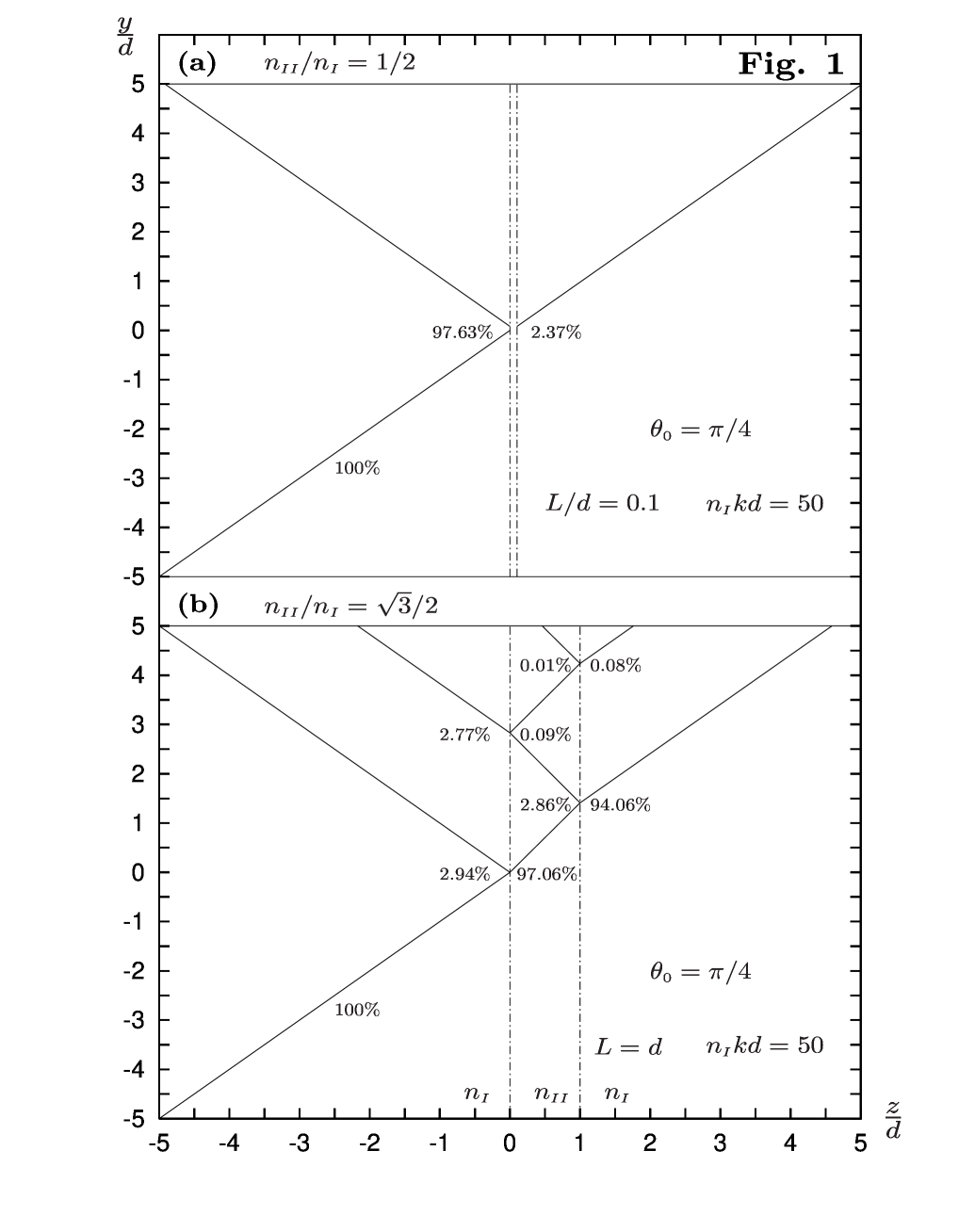
Figure 1: Tunneling (a) and diffusion (b) of a localized optical beam by a dielectric film. The localization is achieved by integrating over the incidence angle (narrow gaussian distribution around the angle $\theta_{\mbox{\tiny$0$}}=\pi/4$). For diffusion phenomena, when the beam localizations are smaller than or of the order of the dimension of region II, we obtain a zebra-like structure, i.e. a multiple diffusion.

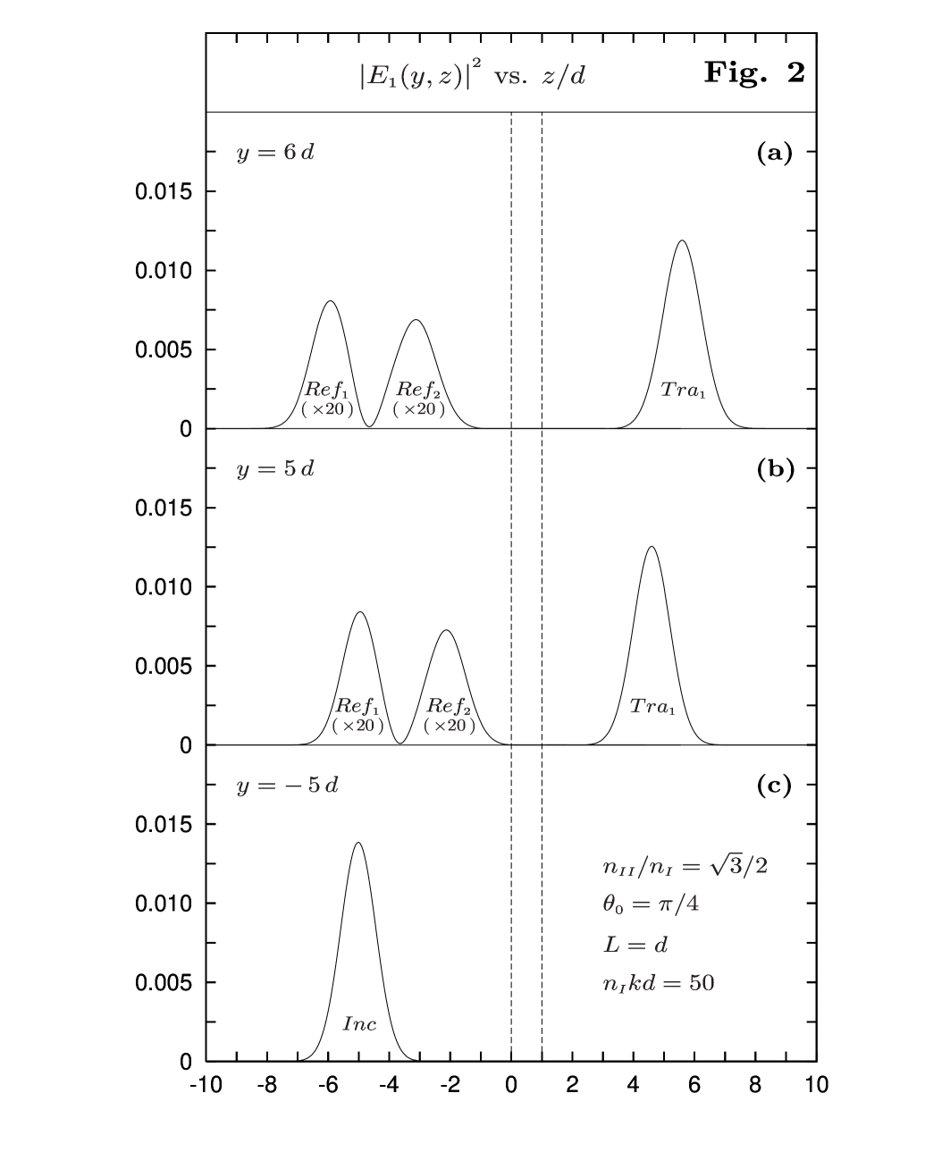
Figure 2: For the diffusion case, the plots of $|E_{\mbox{\tiny$1$}}|^{{}^{2}}$ against $z$ for fixed $y$ show the multiple beams and the localization in the $z$-axis.

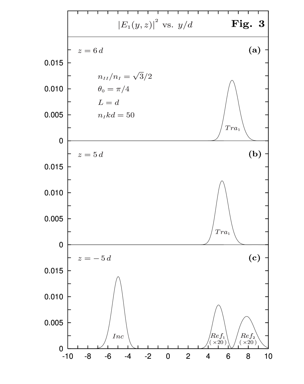
Figure 3: For the diffusion case, the plots of $|E_{\mbox{\tiny$1$}}|^{{}^{2}}$ against $y$ for fixed $z$ show the multiple beams and the localization in the $y$-axis.

References

- [1] A. Bernardini, S. De Leo and P. Rotelli, Mod. Phys. Lett. A 19, 2717 (2004).
- [2] S. De Leo and P. Rotelli, Phys. Lett. A 341, 294 (2005).
- [3] T. E. Hartman, J. Appl. Phys. 33, 3427 (1962).
- [4] V. S. Olkhovsky, E. Recami and J. Jakiel, Phys. Rep. 398, 133 (2004).
- [5] S. De Leo, C. Nishi and P. Rotelli, Int. J. Mod. Phys. A 19, 677 (2004).
- [6] A. Bernardini and S. De Leo, Phys. Rev. D 70, 022101 (2004).
- [7] M. Born and E. Wolf, Principles of optics, Cambridge UP, Cambridge (1999).
- [8] F. Abelés, Ann. de Physique 5, 596 (1950).
- [9] C. Cohen-Tannoudji, B. Diu and F. Laloë, Quantum mechanics, John Wiley & Sons, Paris (1977).
- [10] A.B. Shvartsburg, V. Kuzmiak and G. Petite, Phys. Rep. 452, 33 (2007).
- [11] S. De Leo and P. Rotelli, Eur. Phys. J. C 46, 551 (2006).
- [12] S. De Leo and P. Rotelli, Phys. Rev. A 73, 042107-7 (2006).
- [13] S. De Leo and P. Rotelli, Eur. Phys. J. C 51, 241 (2007).