Highly efficient sparse-matrix inversion techniques and average procedures applied to collisional-radiative codes

Abstract

The behavior of non-local thermal-equilibrium (NLTE) plasmas plays a central role in many fields of modern-day physics, such as laser-produced plasmas, astrophysics, inertial or magnetic confinement fusion devices, or X-ray sources. The proper description of these media in stationary cases requires to solve linear systems of thousands or more rate equations. A possible simplification for this arduous numerical task may lie in some type of statistical average, such as configuration or superconfiguration average. However to assess the validity of this procedure and to handle cases where isolated lines play an important role, it may be important to deal with detailed levels systems. This involves matrices with sometimes billions of elements, which are rather sparse but still involve thousands of diagonals. We propose here a numerical algorithm based on the LU decomposition for such linear systems. This method turns out to be orders of magnitude faster than the traditional Gauss elimination. And at variance with alternate methods based on conjugate gradients or minimization, no convergence or accuracy issues have been faced. Some examples are discussed in connection with the krypton and tungsten cases discussed at the last NLTE meeting. Furthermore, to assess the validity of configuration average, several criteria are discussed. While a criterion based on detailed balance is relevant in cases not too far from LTE but insufficient otherwise, an alternate criterion based on the use of a fictive configuration temperature is proposed and successfully tested. It appears that detailed calculations are sometimes necessary, which supports the search for an efficient solver as the one proposed here.

1 Introduction

Plasmas in a non local thermodynamic equilibrium (NLTE) state play an important role in several domains of physics, such as in astrophysics, in magnetic and inertial confinement devices, in radiation-solid target interaction experiments at large laser facilities, or in XUV and X-rays sources[1, 2]. The proper calculation of important quantities such as the opacity or the emission efficiency requires an accurate atomic physics description of the active medium. In time-independent regimes this implies to solve large systems of kinetic equations describing the population transfers between each level. Several codes have been developed to deal with NLTE plasmas, among which ATOMIC [3], SCROLL [4], MOST [5], ATOM3R [6], AVERROES [7], FLYCHK [8], CRETIN [9], NOMAD [10], JATOM [11], SCAALP [12]. The NLTE meetings provide an opportunity to benchmark them [13, 14, 15, 16].

Because of its inherent complexity, NLTE physics, even in its stationary form, lies on efficient linear algebra algorithms. In our previous approach to this subject [17], we relied on the standard Gauss algorithm: it proves to be very stable and accurate for systems up to several thousand equations, but it becomes prohibitively slow above. A possible workaround to this issue is to resort to statistical averages, the simplest being the configuration average (CA), or the superconfiguration average. A discussion of these averaging procedure efficiency may be found in the literature (e.g., [18]). However, using this average one may neglect important properties, for instance when the various levels in a given configuration have very different excitation rates.

This paper investigates two complementary directions to allow the treatment of complex NLTE plasmas. First, we discuss various possible matrix-inversion algorithms, this step usually being the bottleneck of the collisional-radiative codes (Sec. 2). Then, in Sec. 3, we review several possibilities aimed at designing a criterion that might efficiently qualify the CA procedure. Secs. 4 and 5 illustrate this discussion by dealing with two cases considered at the last NLTE meeting[16]. Brief concluding remarks are given in Sec. 6.

2 Comparison of sparse-matrix inversion techniques

2.1 System properties

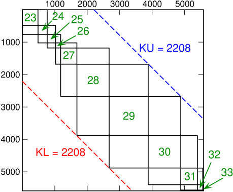
Figure 1: Collisional-radiative rate matrix structure: an example in krypton at $T_{e}=1000\text{ eV}$ and $N_{e}=10^{14}\text{ e/cm}^{3}$. The number of equations is here 5586. The net ion charge is indicated for each diagonal bloc. The cumulated number of levels is indicated in abscissa and ordinate. The broken lines are the sub- and super-diagonal boundaries used in the LU decomposition.

In order to properly characterize plasma properties, including observables as simple as the average net ion charge, one needs to account for a large set of ionic states, including series of doubly or even multiply excited states. This implies that the rate matrices describing the radiative and collisional transfers in such plasmas may have a huge number of elements. Because usually the only transition processes considered in collisional-radiative systems induce a net charge variation $\Delta Z^{*}=0,\pm 1$, these matrices have a tridiagonal-block structure as shown in Fig. 1. If a lot of $Z^{*}$ are considered together, and if the numbers of levels considered for each ion are similar, the matrix contains a large proportion of zeroes and is thus reasonably sparse. Even more, inside the tri-diagonal blocs, some transition rates may cancel (such as those between multiply and singly excited states). However the algorithms proposed here do not account for such zeroes inside the tri-diagonal blocs. A direct estimate in a krypton case illustrated by Fig. 1 revealed that 30 to 40% of such elements do cancel: for this $5586\times 5586$ matrix, with $3.1\times 10^{7}$ elements, $1.2\times 10^{7}$ are in diagonal blocs, which contain themselves $3.8\times 10^{6}$ (32%) “accidentally” null elements. However, dealing properly with such “accidental” cancelation requires to use a cumbersome indexing scheme which may slow down computations, and such attempt was not made in the present work. Clearly this sparse character is stronger when many charge states are included and when each bloc has approximately the same size.

2.2 Gauss algorithm

The first algorithm used to solve collisional-radiative systems is the standard Gauss-Jordan elimination. We could check that this method provides in all considered cases a fair numerical accuracy: this can be done for instance by canceling the unbalanced transition rates and by controlling the level-population departure from the Saha-Boltzmann solution [17]. Except when one pivot accidentally cancel — which was never observed in properly defined NLTE cases — the algorithm always provide a solution, through a constant number of operations, which scales as the cube of the number of equations. To sum up, the Gauss elimination is robust, accurate, but it is really slow and does not take benefit from the sparse character of the system. It will be used only when we consider small systems — as those in configuration average discussed below — or when we wish to cross-check other algorithms.

2.3 Conjugate gradients methods

Conjugate Gradients (CG) methods are iterative procedures for solving a linear system through a series of analytically defined steps. The biconjugate gradient method generalize the procedure to non symmetric definite positive matrices. The convergence of the process may be linked to the use of a preconditioner as discussed, e.g., in [19] and will not be considered here. In this paper our goal is to check how standard routines widely available perform, evaluating their general robustness regardless of the many variants that exist. One must notice that, at variance with [19] where non-stationary systems with few hundreds of levels were included, one may deal here with several tens of thousands of equations. Using CG methods — here we use linbcg from Numerical Recipes [20] — one benefits from the sparse character of the rate matrix since the user is supposed to provide an efficient way to perform the matrix by column vector product.

It appears that the CG codes with no preconditioner may poorly work. As seen below, such iterative methods start on a user-defined solution, and the convergence may strongly depend on this step. Besides a convergence criterion must be chosen. It was found that the inline criterion included with linbcg routine is not satisfactory: The proposed error parameter may be still about 1 while convergence has indeed be reached. Therefore in this work we used the natural and physically sound criterion based on the average net charge $Z^{*}$ variation for the last two iterations. Namely, when for the first time

$$|<Z^{*}>_{n}-<Z^{*}>_{n-1}|\leq\varepsilon\text{\quad and\quad}|<Z^{*}>_{n}-<Z^{*}>_{n-2}|\leq\varepsilon$$ (1)

with for instance $\varepsilon=10^{-7}$ convergence is assumed to be reached. Two steps are considered since it appeared that a single check could produce an artificial convergence.

As shown below (subsection 2.5), the CG methods when they converge are fast and accurate. However, the CG algorithm may lack of robustness. For instance, we considered the case where radiative and autoionization rates are canceled: including only the collisional excitation and ionization and the reverse processes, and comparing the solution with Saha-Boltzmann is a way to check the algorithm accuracy [17]. In a krypton plasma at a 500 eV temperature and $10^{14}\text{ cm}^{-3}$ electronic density, with 5 662 levels and 14 charge states accounted for, we did obtain populations different from Saha-Boltzmann by $2\times 10^{-13}$ in average ($6\times 10^{-10}$ at maximum), but this was obtained after a rather large number of iterations: 1966 with $\varepsilon=10^{-13}$ in Eq. (1), starting with zero populations. The inspection of $<Z^{*}>$ before convergence shows strong fluctuations from one iteration to the next. One may estimate that the condition $\varepsilon=10^{-13}$ is too severe, which overestimate the convergence effort, but if one stops the process at, e.g., 150 iterations as obtained in well behaved cases (see next paragraphs), the $<Z^{*}>$ fluctuations on the last iterations are above $10^{-3}$, which is unacceptably large.

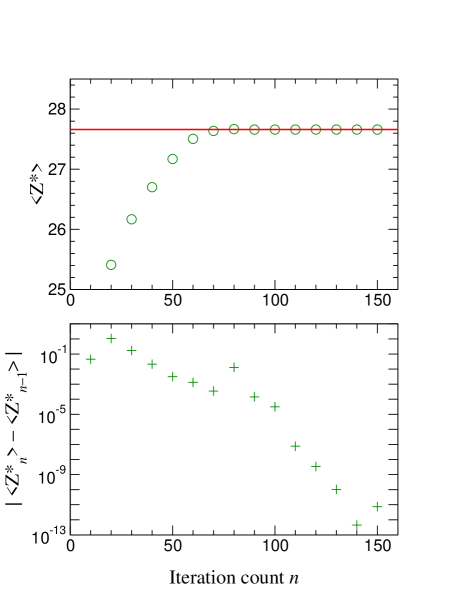
Figure 3: Same as Fig. 2 but starting on zero populations.

Moreover, as for every iterative process, the CG convergence may depend on the initial choice for the populations. To illustrate this when no preconditioner is used, we have plotted in Fig. 2 and Fig. 3 results of a NLTE analysis in krypton for an electronic temperature of $T_{e}=1000\text{ eV}$ and an electronic density of $N_{e}=10^{14}\text{ cm}{-3}$. Here the number of equations is $N=5586$, large enough to check significantly the calculation speed, but still moderate to allow direct computation by the slow but stable Gauss elimination. The linbcg internal convergence criterion gives an “error” of 3.3 after 140 iterations and 19.6 after 150 iterations, while it is obvious from Fig. 3 that convergence does then occur. One notices that initializing the process with zero populations give fast and accurate convergence: 150 steps if accuracy of $10^{-12}$ on $<Z^{*}>$ is sought as indicated by the lower part of Fig. 3; The otherwise known correct $<Z^{*}>$ is given by the horizontal line in the upper figure.

Conversely, initialization on Saha-Boltzmann populations leads to an erratic behavior. After about 4000 steps one gets close to the correct solution but with a mediocre $10^{-3}\text{--}10^{-5}$ accuracy (cf. lower Fig. 2). Then the solution begins to diverge and reaches after almost 10 000 iterations a “false convergence” at $<Z^{*}>\simeq 28.162$, significantly off the (otherwise confirmed) Gauss solution of $<Z^{*}>=27.660$. Up to 25 000 iterations have been performed here. The $<Z^{*}>$ variation from one step to the next as seen on the lower part of Fig. 2 remains above $10^{-7}$: The fact that this figure is much greater than machine accuracy $\simeq 10^{-16}$ indicates that this “convergence” is not satisfactory. This further indicates that the $\varepsilon$ parameter of criterion (1) must be chosen very carefully.

2.4 LU decomposition

Another possible choice for matrix inversion is based on the LU decomposition algorithm, which uses an upper-lower triangular matrix decomposition. The used routine is here dgbsvx from lapack linear algebra package, which assumes a band-diagonal structure for the matrix to be inverted. The balancing of rows and columns is automatically done inside the code. The matrix condition is checked and given as an output parameter; In the various cases tested, at or far from thermal equilibrium, it was found to be satisfactory. In addition to the storage of the original matrix with $K_{L}$ and $K_{U}$ lower and upper diagonals, which occupies $(K_{L}+K_{U}+1)\times N$, $N$ being the number of equations, the proposed algorithm requires the storage of the lower and upper triangular matrices, i.e., $(2K_{L}+K_{U}+1)\times N$ additional memory locations. Considering realistic values for the $K_{L}$ ($=K_{U}$) parameter, this amounts to foresee storage as large as 32 GB for a matrix size $N\simeq 50~{}000$.

The various tests performed have shown that this algorithm is fast, accurate and robust. No particular row or column balancing had to be done by a preprocessor, since this is automatic in the lapack routine. The matrix condition is checked inside the code and it was found satisfactory in every considered cases. As an accuracy test proposed before [17], we solved with the LU algorithm a kinetic system of 4481 equations including only collisional excitation, collisional ionization plus the reverse processes. One gets then the Saha-Boltzmann solution with a maximum population difference of $1.2\times 10^{-12}$, and an average difference of $5.4\times 10^{-16}$, the Gauss algorithm providing the same excellent accuracy. It appears that the only serious limitation to LU method is the storage issue, even for reasonably sparse matrices. Looking again at Fig. 1, the stored elements are all those between the upper and lower broken lines, and additional storage is needed for the lower and upper triangular matrices too.

2.5 Relative efficiency of the algorithms

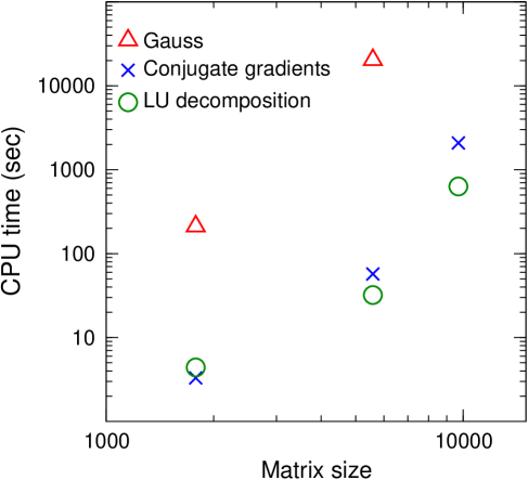
Figure 4: Computation time for matrix inversion using standard Gauss algorithm, a conjugate gradient code, and LU decomposition.

Examples of elapsed CPU time for the three methods are given in Fig. 4. Three NLTE cases of “physical interest” are illustrated here: carbon at 10 eV and $10^{12}\text{ e.cm}^{-3}$ with the 7 charge states and about 1800 levels, krypton at 1 keV and $10^{14}\text{ e.cm}^{-3}$ with Krxxiv–xxxiv ions and about 5600 levels included, and at 200 eV, $10^{22}\text{ e.cm}^{-3}$ with Krxix–xxviii ions and about 9700 levels included. In the last case, the kinetic system was too large to allow ourselves for a resolution by the Gauss algorithm in a reasonable time. It appears that while computation time increases rapidly with the matrix size, the CG and LU methods are orders of magnitude faster then Gauss elimination. Because as seen above the tested CG algorithm lacks of robustness, the preferred LU method is used in all the computations presented below.

3 Configuration-average procedures and validity criteria

Configuration average (CA) procedures have been discussed in previous papers [18, 17, 21]. It is the simplest and more natural way to considerably alleviate the matrix inversion task involved in stationary NLTE cases, and, interestingly enough, it usually provides rather accurate results.

3.1 Configuration average(s)

Assuming the ionic level $i$ (resp. $j$) belongs to configuration $\alpha$ (resp. $\beta$) the average rate from $\alpha$ to $\beta$ is

$$R_{\alpha\beta}=\frac{1}{g_{\alpha}}\sum_{\begin{subarray}{c}i\in\alpha\\ j\in\beta\end{subarray}}g_{i}R_{ij},\text{\quad with\ }g_{\alpha}=\sum_{i\in\alpha}g_{i}$$ (2)

where $g_{i}$ is the $i$-level degeneracy, and $g_{\alpha}$ is the configuration degeneracy. We can set an alternate definition by including the Boltzmann factor

$$R_{\alpha\beta}=\left.\sum_{\begin{subarray}{c}i\in\alpha\\ j\in\beta\end{subarray}}g_{i}\exp(-E_{i}/(k_{B}T_{e}))R_{ij}\right/\sum_{i\in\alpha}g_{i}\exp\left(-E_{i}/(k_{B}T_{e})\right),$$ (3)

which can be assumed more “accurate” because the levels inside a given configuration usually have neighboring energies and are likely to fulfill thermal equilibrium. Of course, corresponding definitions hold for the average energies, energy rms, etc.

Another option that generalizes both previous ones consists in arbitrarily defining some “configuration temperature”, i.e.,

$$R_{\alpha\beta}=\left.\sum_{\begin{subarray}{c}i\in\alpha\\ j\in\beta\end{subarray}}g_{i}\exp(-E_{i}/(k_{B}T_{c}))R_{ij}\right/\sum_{i\in\alpha}g_{i}\exp\left(-E_{i}/(k_{B}T_{c})\right),$$ (4)

where $T_{c}$ can be freely chosen. The dependence of the various physical quantities on the choice of $T_{c}/T_{e}$ will qualify the CA validity, as will be illustrated in the next sections, in cases where CA holds or does not hold.

3.2 Validity criteria

These CA formula being defined, it is important to elaborate a criterion that can properly qualify the relevance of this procedure, of course avoiding to go back to the time-consuming detailed level analysis.

3.2.1 The natural criterion based energy dispersion

The most intuitive criterion for the validity of CA may be written as

$$<\Delta E>=\sum_{\alpha}N_{\alpha}\Delta E_{\alpha}\ll k_{B}T_{e}$$ (5)

where $N_{\alpha}$ is the $\alpha$-configuration population (with $\sum_{\alpha}N_{\alpha}=1$) and $\Delta E_{\alpha}$ the energy dispersion

$$\Delta E_{\alpha}=\left(\frac{1}{g_{\alpha}}\sum_{i\in\alpha}g_{i}(E_{i}-E_{\alpha})^{2}\right)^{1/2}.$$ (6)

This criterion is fairly easy to implement, since it only requires to solve once a simple CA kinetic system. However, as stressed before [17] and checked once more here (see, e.g., subsection 5.3), this necessary condition is far from being sufficient, a plain reason being that it involves a strongly averaged quantity, which furthermore depends on level energies and not on transition rates that can vary significantly inside a given pair of configurations.

3.2.2 A criterion based on LTE test and its applicability range

A criterion based on the comparison between the Saha-Boltzmann solution and of the solution of a partial rate kinetic equation has been proposed in previous papers [17, 21]. It consists in checking how well the CA of a system containing rates that obey detailed balance — collisional rates in [17], any rates in [21] — reproduces the Saha-Boltzmann solution. In more detail, one first evaluates using (2) average collisional rates $R^{\prime}_{\alpha\beta}$ where the rates $R^{\prime}$ include only the collisional excitation, the collisional ionization, and the reverse processes. Then one solves the CA kinetic system

$$\frac{dN_{\alpha}}{dt}=-\sum_{\begin{subarray}{c}\beta\\ \beta\neq\alpha\end{subarray}}R^{\prime}_{\alpha\beta}N_{\alpha}+\sum_{\begin{subarray}{c}\beta\\ \beta\neq\alpha\end{subarray}}R^{\prime}_{\beta\alpha}N_{\beta}=0$$ (7)

that gives the configuration populations $N_{\alpha}$. Last, one compares this solution with the Saha-Boltzmann populations of the configurations $N^{\text{SB}}_{\alpha}$. Since the $R^{\prime}$ rates obey detailed balance, the difference $N_{\alpha}-N^{\text{SB}}_{\alpha}$ is a measure of the validity of CA. This criterion has proven to give good results in a carbon plasma at 3 eV or 10 eV [17].

However we must point some drawbacks of this approach. First, the criterion in its simplest form relies on a comparison of average net charges, which is known to be rather insensitive to the detail of the populations, regarding excited levels for instance. Second and more seriously, this criterion checks the CA validity close to LTE, and, if the studied situation is significantly far from LTE, it cannot be predictive. Examples in this direction will be provided in next sections. This criterion appears as necessary but not sufficient either.

3.2.3 An alternate criterion based on fictive configuration temperatures

A last approach consists in solving the CA kinetic equations using the various averages [Eqs. (2), (3), (4)] and to compare the results. The comparison may concern several physical quantities such as $<Z^{*}>$, the radiative bound-bound rate

$$P_{\text{bb}}=N_{\text{ions}}\sum_{i}p_{i}\sum_{j}(E_{i}-E_{j})A_{ij}$$ (8)

$p_{i}$ being the $i$-level population, $E_{i}-E_{j}$ the transition energy, and $A_{ij}$ the radiative rate, or the radiative bound-free rate. This criterion requires to solve at least two CA systems, and preferably three, one at $T_{c}$ infinite, one at $T_{c}=T_{e}$, and one at a fictive low $T_{c}$, e.g., $0.1T_{e}$. Examples will be given in the next sections.

4 The krypton case: validity and limitation of CA

The analysis of charge distribution and radiative losses in krypton presents a definite interest for various reasons. Krypton is used in numerous plasmas devices, and one must mention the availability of radiative loss measurements by Fournier et al [22].

The present study deals with temperatures at least equal to 500 eV, and electron densities up to $10^{22}\text{ cm}^{-3}$, charge states from XIX to XXXVII are accounted for. For such large temperatures, the collisional rates are low enough to provide a strongly non-LTE situation. The configurations included in the computation are listed in Table Tables. In order to include an important set of excited states required for a pertinent description, this list is much more complete than the one considered for test purposes in Sec. 2. For instance at 1 keV, $10^{14}\text{ e/cm}^{3}$, the present computation includes 45 927 levels vs 5 587 previously. The energy and rate computations in krypton as well as in tungsten are performed using the HULLAC suite [23].

This accounts for a large number of autoionizing configurations while keeping the NLTE computation tractable even in the detailed case. Lower temperatures would require a more complete set of ions but are within the reach of present method.

The average charge, the radiative bound-bound (bb) losses and the radiative bound-free (bf) losses are plotted in Fig. 5 and 6 for electronic densities equal to $10^{14}$ and $10^{18}\text{ cm}^{-3}$ respectively. Detailed computation and configuration average results are both displayed. Once again, the agreement between both computations is good. This is particularly true at $T=1000\text{ eV}$ and $T=5000\text{ eV}$ where the average charge is close to, respectively, 26 and 34, which corresponds to the Ne-like and He-like closed shell ions. Then it is well known that all computations tend to give agreeing predictions.

Since Fournier et al performed measurements of the radiative cooling coefficient in coronal Kr plasmas [22], it is instructive to compare our $10^{14}\text{ cm}^{-3}$ data to theirs. The radiative cooling coefficient is defined for coronal plasmas as

$$L^{\text{tot}}=<Z^{*}>(P_{\text{bb}}+P_{\text{bf}}+P_{\text{ff}})/N_{e}^{2}$$ (9)

where $P_{\text{ff}}$ is the Bremsstrahlung loss rate, which we can derive from the approximate expression (formula 4.24.4 in [24])

$$P_{\text{ff}}\text{(erg/s/cm${}^{3}$)}\approx 5.35\times 10^{-24}<Z^{*}>N_{e}^{2}(T_{e})^{1/2}\text{ with $N_{e}$ in cm${}^{-3}$, $T_{e}$ in keV.}$$ (10)

More accurately, we should substitute $<Z^{*}{}^{2}>/<Z^{*}>$ to $<Z^{*}>$ in the rate (10) but this looks unnecessary since this is just an estimation. At 1 keV and $10^{14}\text{ e.cm}^{-3}$, the ff term is $P_{\text{ff}}\simeq 1.4\times 10^{6}\text{ cgs}$, less than the bf one and quite small with respect to the bb contribution.

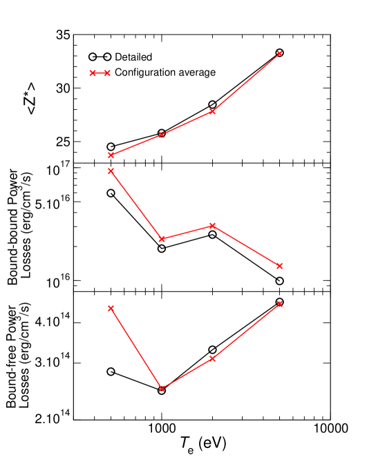
Figure 6: Same as Fig. 5 but for an electronic density of $10^{18}\text{ cm}^{-3}$.

From Fig. 6 of Ref.[22], we get a radiative coefficient $L^{\text{tot}}=6\times 10^{-32}\text{ W.m}^{3}$ at 1 keV, while the present determination is $7.8\times 10^{-32}$, in very good agreement if we consider the difficulty of this measurement. At 500 eV, the agreement deteriorates ($1.6\times 10^{-31}\text{ SI}$ measured, vs. $5.9\times 10^{-31}$ computed), while at 2 keV one gets again fair agreement ($6\times 10^{-32}$ measured vs $8.6\times 10^{-32}$ obtained here).

A clear discrepancy between detailed and configuration average is visible on the bound-free losses at 500 eV and $10^{18}\text{ cm}^{-3}$: $2.82\times 10^{14}\text{ erg/s/cm}^{3}$ in the detailed model, $4.43\times 10^{14}\text{ erg/s/cm}^{3}$ in CA. Nevertheless this bf-loss ratio does not exceed 1.57, and bound-free losses are two orders of magnitude lower than bound-bound losses, which means that such a difference will hardly be noticed experimentally, only the sum being measured. However, one may try to look closer at the origin of this discrepancy. A first explanation could come from the averaging procedure that can include or not the Boltzmann factor (Eqs. 3, 2), the Fig. 6 corresponding to the case including the Boltzmann factor. The inspection of Table 2 demonstrates that the averaging procedure is not at stake. For all the plotted data, both configuration-average quantities would be indistinguishable at the drawing accuracy. One simply notices that the agreement between both averages increases with $T_{e}$, as expected.

A more thorough analysis arises from the detailed analysis of the radiative losses contributions. The configurations contributing the most to bound-free losses according to the CA calculations are listed in Table 1. One may see that, e.g., the $1s^{2}2s^{2}2p^{6}3p3d$ configuration of $\text{Kr}^{24+}$ dominates for the bf losses in the CA computation (total population 0.0147, contribution to bf losses $2.48\times 10^{14}\text{ erg/s/cm}^{3}$), while the corresponding levels contribute for a population of 0.0219 and bf losses of $5.13\times 10^{13}\text{ erg/s/cm}^{3}$ in the detailed computation.

Conversely, in the detailed scheme, the level contributing the most to bf losses is the Kr²⁵⁺ ground level ($8.46\times 10^{13}\text{ erg/s/cm}^{3}$), followed by the Kr²⁴⁺ $(1s^{2}2s^{2}2p^{6})^{1}S_{0}3p_{1/2}3d_{5/2}J=3$ level ($4.68\times 10^{13}$) and Kr²⁶⁺ Ne-like ground level ($4.65\times 10^{13}$).

As a rule one notices that a detailed inspection (e.g., at the configuration level) of populations or radiative losses may reveal large discrepancies between models that will remain hidden when only global quantities are considered.

To check how the CA validity criteria defined in subsection 3.2.3 behaves, we have done two additional computations of the Kr plasma properties in configuration average. One was performed using the “infinite configuration temperature” scheme as defined by formula (2), while the last one used a finite temperature (4) chosen below the electronic temperature $T_{c}/T_{e}=0.1$. The results of the various CA compared to the detailed computation are shown in Table 2. It appears that the average (4) agrees usually within 2% or better with (2), except on bf losses at 500 eV, where the difference exceeds 5%. This discrepancy is an indication of the (stronger) difference between the CA and detailed values. A computation with $T_{c}/T_{e}=0.01$ would increase this difference.

5 The tungsten case: an example of configuration-average validity breakdown

Tungsten exhibits some interesting properties that qualify it for being one of the constituents of the divertor in modern tokamaks [25]. It presents a high melting point, a low erosion rate, and a low tritium retention. However, in such a plasma one may expect high radiative losses because of the richness of its spectrum. It also allows to benchmark X-ray spectrum calculations [26]. That is why tungsten was in the list of cases submitted to the NLTE-5 workshop [16].

5.1 Description of the computation

The list of configurations used in the present computation is similar to the one used in krypton (Table Tables). The computations performed here are restricted to $T_{e}=20\text{ keV}$ and 30 keV, at a density of $N_{e}=10^{14}\text{ cm}^{-3}$. The density $10^{24}\text{ cm}^{-3}$ was also considered, but since the present model does not account for continuum lowering (or pressure ionization), these results are not really significant and could be exploited only if compared to alternate models. The net charge states included are 59–72 and 61–74 for $T_{e}=20\text{ keV}$ and 30 keV respectively (at $10^{24}\text{ cm}^{-3}$, 60–74 and 61–74 charges were considered).

5.2 Average charge and radiative losses analysis

Results are summarized in Table 3. Considering the $<Z^{*}>$ value, we check that detailed and configuration-average computations provide similar figures: at 20 keV one gets 65.004 and 64.547 respectively, and at 30 keV, 67.389 and 67.265, where the CA is performed using Boltzmann ponderation as defined in (3). The bound-free radiative losses, mostly sensitive to the ground-state population of each ions, are also quite similar in both computations. However, a huge discrepancy is observed on the bound-bound radiative losses, since at 30 000 eV the computed figures are $4.866\times 10^{7}$ and $6.496\times 10^{13}$ erg/s/cm³ in the detailed and CA cases respectively.

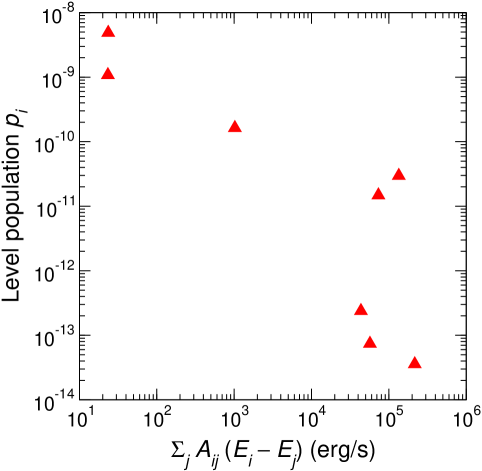
Figure 7: Radiative losses from and populations of the eight levels belonging to the $1s^{2}2s2p^{2}$ configuration of $W^{69+}$. The lower levels $j$ of the radiative decay belong to the $1s^{2}2s^{2}2p$ configuration. The detailed level computation is done at 30 000 eV and $10^{14}\text{ e/cm}^{3}$.

This surprising feature cannot be explained by a drastic variation of the charge distribution, rather similar in both cases. To trace the origin of this discrepancy, one must resort to a finer analysis of the contributions of each pair of configurations to the bound-bound rate. Doing this, it appears that the huge bound-bound losses in CA case originate mostly from the transition between the $1s^{2}2s^{2}2p$ and the $1s^{2}2s^{2}2p$ configurations of the Wlxx ion. While the former configuration exhibits a plain fine-structure splitting of the $2p$ doublet (of about 1500 eV, which much less than the electronic temperature), the latter one has a more complex structure. It contains 8 levels, the 5 lowest ones being at energies close to one of the $1s^{2}2s^{2}2p$ doublet component, while the 3 upper levels are approximately 1700 eV above the $2p_{3/2}$ upper component of the doublet. The two configuration levels therefore strongly overlap. Considering the radiative deexcitation rates, a detailed inspection demonstrates that the 5 higher levels of the $1s^{2}2s^{2}2p$ configuration exhibit the largest radiative rates (above $10^{13}\text{ s}^{-1}$), while they are noticeably the less populated. This fact is illustrated by Fig. 7, where the eight level populations $p_{i},i\in 1s^{2}2s2p^{2}$ as obtained from the detailed computation are plotted in ordinate while the abscissas stand for the individual radiative loss factor $\sum_{j\in 1s^{2}2s^{2}2p}A_{ij}(E_{i}-E_{j})$. The anticorrelation between populations and rates appear strikingly on this plot. An additional explanation for the inadequacy of the CA computation in this case comes from the total population of the $1s^{2}2s2p^{2}$ configuration. The CA computation gives $\simeq 4\times 10^{-3}$, while the sum of the eight level populations in the detailed approach is only $\simeq 3\times 10^{-8}$, lowering thus the radiative bound-bound losses by 5 orders of magnitude. The discrepancy on this configuration population originates also from significant variations in the collisional and radiative detailed rates between configurations, and it has not been analyzed in more detail.

5.3 About various criteria assessing the validity of configuration average

One must now consider whether this strong discrepancy was expected, since the CA average remain much less computer-time consuming.

First the plain criterion on the average energy dispersion is pointless here: one computes for the energy rms inside each configuration ponderated by its population (5) $<\Delta E>=625\text{ eV}$, far below $T_{e}=30~{}000\text{ eV}$. Then, the criterion of subsection 3.2.2 based on the comparison of the Saha-Boltzmann solution with the CA solution of a modified rate equation is of no help either. The temperature being very high (and the density very low), the modified rate equations give a plain fully ionized plasma, the $Z^{*}<74$ ion population being less than $10^{-7}$. This solution is in excellent agreement with Saha-Boltzmann equation, but provides no relevant information on the real plasma, far from thermal equilibrium.

One must then resort to the fictive-configuration-temperature criterion devised in subsection 3.2.3. The use of this criterion is illustrated in Table 3. Therefore, in addition to the detailed computation, we have performed the three configuration averages proposed in Sec. 3. The first average (2) is the $g$ ponderation, i.e., the infinite temperature limit; the “natural” average (3) involving Boltzmann factors corresponds to the previously discussed CA value. For the “fictive configuration temperature” case (4) one has taken $T_{c}/T_{e}=0.1$, in order to test $T_{c}$ well above and below $T_{e}$.

Considering first the $Z^{*}$ average, comparing the CA data obtained with an infinite temperature (column 3) with the data with low $T_{c}$ (column 5, the column 4 being in between), one checks that these two figures are close. If we look now at the b-b losses (columns 6–9), we see that (2), or (3) which is close, differ by almost a factor of 2 at 20 000 eV, and less but still significantly at 30 000 eV. This discrepancy between averages (2) and (4) must be interpreted as a failure of the configuration average, i.e., is a clue of the even much stronger discrepancy between the detailed result and the (3) average. Once again, the interesting fact in using (2) and (4) is that this requires only two quite fast configuration average computations to check whether a detailed analysis is required. Moreover, looking at $Z^{*}$, bound-bound and bound-free losses in this table, one notices immediately that only the bound-bound figure in CA formalism is highly dubious.

In order to validate further the $T_{c}$ criterion, we also performed computations with $T_{c}/T_{e}=0.01$. It appears that, at 20 000 eV, one gets $<Z^{*}>=64.362$ with $T_{c}=200\text{ eV}$, not too different from the $T_{c}\infty$ limit, which strengthen our confidence in this CA average. Conversely, in the same conditions, the bound-bound losses are $2.2\times 10^{9}\text{ erg/s/cm}^{3}$ to be compared to the $T_{c}$-infinite CA value of $1.3\times 10^{13}\text{ erg/s/cm}^{3}$: This huge change clearly indicates a failure of the CA approximation when dealing with bb losses. Once again, the modest variation of the bound-free losses ($8.48\times 10^{6}\text{ erg/s/cm}^{3}$ to $8.60\times 10^{6}\text{ erg/s/cm}^{3}$ when $T_{c}$ varies from $T_{e}/100$ to $\infty$) insures that such observable is reasonably computed within CA approximation.

6 Conclusions

Reliable computations of plasma properties significantly out of local thermal equilibrium involving complex atoms require to solve large linear systems, for which various algorithms have been tested. Without claiming exhaustivity, it appears that the LU decomposition method offers a good compromise regarding stability, robustness, accuracy and computation speed. Alternate methods using, e.g., conjugate gradients with a preconditioner are worth consideration but certainly of less direct usage. We have investigated a second direction to simplify the kinetic system solution, based on configuration average. In addition to the already known criteria, that provide a necessary but not sufficient condition, we have tested a criterion based on the use of a fictive configuration temperature. This criterion proves to be very efficient including when dealing with situations far off thermal equilibrium. Moreover, even negative configuration temperatures may be used, allowing a vast range of configuration average checking. Since in some situations, as illustrated by the bound-bound power losses in tungsten at high $T_{e}$, this average performs poorly it is essential to use an efficient validity criterion and when necessary to dispose of a fast and robust algorithm for the very large kinetic systems that must then be solved.

Tables

[thb] Ion $N_{c}$ $N_{l}$ List of configurations KrXIX 70 3781 $[1s^{2}2s^{2}2p^{6}]3s^{2}3p^{5}nl$, $3s^{2}3p^{4}3dnl$, $3s3p^{6}nl$, $3p^{6}3dnl$; $1s^{2}2s^{2}2p^{5}3s^{2}3p^{6}nl$, $1s^{2}2s2p^{6}3s^{2}3p^{6}nl$ KrXX–XXII $(N=4,3,2)$ 63 ^a $[1s^{2}2s^{2}2p^{6}]3s^{2}3p^{N}nl$, $3s^{2}3p^{N-1}3dnl$, $3s3p^{N+1}nl$; $1s^{2}2s^{2}2p^{5}3s^{2}3p^{N}nl$, $1s^{2}2s2p^{6}3s^{2}3p^{N}nl$ KrXXIII 80 6006 $[1s^{2}2s^{2}2p^{6}]3s^{2}3pnl$, $3s^{2}3dnl$, $3s3p^{2}nl$, $3s3p3dnl$, $3p^{3}nl$, $3p^{2}3dnl$; $1s^{2}2s^{2}2p^{5}3s^{2}3p^{2}nl$, $1s^{2}2s2p^{6}3s^{2}3p^{2}nl$ KrXXIV 75 2239 $[1s^{2}2s^{2}2p^{6}]3s^{2}n$l, $3s3pnl$, $3s3dnl$, $3p3dnl$; $1s^{2}2s^{2}2p^{5}3s^{2}3pnl$, $1s^{2}2s2p^{6}3s^{2}3pnl$ KrXXV 61 1499 $[1s^{2}2s^{2}2p^{6}]3snl$, $3pnl$, $4l4l^{\prime}$, $1s^{2}2s^{2}2p^{5}3l3l^{\prime}3l^{\prime\prime}$; $1s2s^{2}2p^{6}3l3l^{\prime}3l^{\prime\prime}$ KrXXVI 67 2129 $1s^{2}2s^{2}2p^{6}nl$, $1s^{2}2s^{2}2p^{5}nln^{\prime}l^{\prime}$, $1s^{2}2s2p^{6}3l3l^{\prime}$; $1s2s^{2}2p^{6}3l3l^{\prime}$ KrXXVII 83 5397 $1s^{2}2s^{2}2p^{5}n$l, $1s^{2}2s2p^{6}nl$, $1s^{2}2s^{2}2p^{4}nln^{\prime}l^{\prime}$, $1s^{2}2s2p^{5}3l3l^{\prime}$, $1s^{2}2p^{6}3l3l^{\prime}$; $1s2s^{2}2p^{6}3l$ KrXXVIII 82 6758 $1s^{2}2s^{2}2p^{4}nl$, $1s^{2}2s2p^{5}nl$, $1s^{2}2s^{2}2p^{3}nln^{\prime}l^{\prime}$; $1s2s^{2}2p^{6}$ KrXXIX 74 4739 $1s^{2}2s^{2}2p^{3}nl$, $1s^{2}2s2p^{4}nl$, $1s^{2}2p^{5}nl$, $1s^{2}2s^{2}2p^{2}nln^{\prime}l^{\prime}$; $1s2s^{2}2p^{5}$, $1s2s2p^{6}$ KrXXX–XXXI $(N=2,1)$ 94 ^b $1s^{2}2s^{2}2p^{N}nl$, $1s^{2}2s2p^{N+1}nl$, $1s^{2}2p^{N+2}nl$, $1s^{2}2s^{2}2p^{N-1}nln^{\prime}l^{\prime}$; $1s2s^{2}2p^{N+2}$, $1s2s2p^{N+3}$, $1s2p^{N+4}$, $1s2s^{2}2p^{N+2}3l$, $1s2s2p^{N+2}3l$, $1s2p^{N+3}3l$ KrXXXII 135 3568 $1s^{2}2s^{2}nl$, $1s^{2}2s2pnl$, $1s^{2}2p^{2}nl$, $1s^{2}2snln^{\prime}l^{\prime}$; $1s2s^{2}2p^{2}$, $1s2s2p^{3}$, $1s2p^{4}$, $1s2s^{2}2p3l$, $1s2s2p^{2}3l$, $1s2p^{3}3l$ KrXXXIII 80 751 $1s^{2}2snl$, $1s^{2}2pnl$, $1s^{2}nln^{\prime}l^{\prime}$; $1s2s^{2}2p$, $1s2s2p^{2}$, $1s2p^{3}$, $1s2s^{2}3l$, $1s2s2p3l$, $1s2p^{2}3l$ KrXXXIV 23 106 $1s^{2}nl$; $1s2s^{2}$, $1s2p^{2}$, $1s2l3l^{\prime}$ KrXXXV 18 59 $1snl$; $2l2l^{\prime}$ KrXXXVI 15 25 $nl$

• $N_{l}=6988,8980,7319\text{ for }N=4,3,2$ respectively

• $N_{l}=3607,1915\text{ for }N=2,1$ respectively

Configurations included in Kr computation. Unless otherwise specified, one has $n\leq 5,l\leq n-1$. When $n$ and $n^{\prime}$ are involved in the same configuration, one has $6\leq n+n^{\prime}\leq 8$ with $l\leq n-1,l^{\prime}\leq n^{\prime}-1$. $N_{c}$ is the number of nonrelativistic configurations, $N_{l}$ the number of levels. In the HULLAC computation, the configurations are usually separated in two groups within which interaction is fully accounted for; these groups are separated by a semicolon in the list, the second group containing excitation of an inner electron ($1s$, $2s$ or $2p$).

$Z$	Configuration	CA: population	CA: bf losses	DL: population	DL: bf losses
			(erg/s/cm3)		(erg/s/cm3)
24	$1s^{2}2s^{2}2p^{6}3p3d$	0.0147	$2.48\times 10^{14}$	0.0219	$5.13\times 10^{13}$
23	$1s^{2}2s^{2}2p^{6}3s^{2}3p$	0.318	$6.02\times 10^{13}$	0.0931	$1.68\times 10^{13}$
25	$1s^{2}2s^{2}2p^{6}3s$	0.157	$4.50\times 10^{13}$	0.305	$8.46\times 10^{13}$
Total		1	$4.43\times 10^{14}$	1	$2.82\times 10^{14}$

Table 1: Configurations with the largest contribution to the radiative bound-free (bf) losses in Kr at 500 eV and $10^{18}\text{ cm}^{-3}$, in the configuration average (CA) case and in detailed level (DL) computation. The total population of the configuration and its contribution to bf losses (erg/s/cm³) is given in each case.

$T_{e}\text{ (eV)}$	$<Z^{*}>$				Bound-bound losses ($10^{16}\text{ erg/s/cm}^{3}$)				Bound-free losses ($10^{14}\text{ erg/s/cm}^{3}$)
(eV)	detailed	(2)	(3)	(4)	detailed	(2)	(3)	(4)	detailed	(2)	(3)	(4)
500	24.516	23.749	23.733	23.586	5.949	9.327	9.332	9.381	2.823	4.406	4.431	4.633
1000	25.786	25.654	25.654	25.650	1.919	2.333	2.331	2.318	2.465	2.495	2.499	2.532
2000	28.457	27.826	27.830	27.860	2.553	3.049	3.053	3.097	3.299	3.095	3.097	3.110
5000	33.297	33.234	33.234	33.234	0.9903	1.347	1.345	1.319	4.638	4.573	4.573	4.573

Table 2: Krypton plasma properties at $10^{18}\text{ e.cm}^{-3}$. The average net charge $<Z^{*}>$, radiative bound-bound and bound-free losses are given in the detailed-level models (columns 2, 6, 10) and in the configuration average approximation. This average is performed using in the Boltzmann factor a configuration temperature $T_{c}$ infinite (Eq. 2), equal to the electronic temperature $T_{e}$ (Eq. 3) or such as $T_{c}=0.1T_{e}$ (Eq. 4).

$T_{e}\text{ (eV)}$	$<Z^{*}>$				Bound-bound losses ($10^{7}\text{ erg/s/cm}^{3}$)				Bound-free losses ($10^{6}\text{ erg/s/cm}^{3}$)
(eV)	detailed	(2)	(3)	(4)	detailed	(2)	(3)	(4)	detailed	(2)	(3)	(4)
$2\times 10^{4}$	65.004	64.541	64.547	64.571	6.370	1.290[6]	1.223[6]	6.766[5]	9.238	8.601	8.606	8.635
$3\times 10^{4}$	67.389	67.263	67.265	67.254	4.866	6.683[6]	6.496[6]	4.866[6]	9.917	9.396	9.399	9.424

Table 3: Same as table 2 but for a tungsten plasma at $10^{14}\text{ e.cm}^{-3}$. The notation 1.290[6] stands for $1.290\times 10^{6}$.

List of Figures

1. 1 Collisional-radiative rate matrix structure: an example in krypton at $T_{e}=1000\text{ eV}$ and $N_{e}=10^{14}\text{ e/cm}^{3}$. The number of equations is here 5586. The net ion charge is indicated for each diagonal bloc. The cumulated number of levels is indicated in abscissa and ordinate. The broken lines are the sub- and super-diagonal boundaries used in the LU decomposition.
2. 2 Average charge (upper figure) and its variation from one step to the previous (lower figure) in Kr as computed with conjugate gradient method starting on Saha-Boltzmann populations. The horizontal red line corresponds to the average charge as determined by the stable Gauss algorithm. The electron temperature and density are 1000 eV and $10^{14}\text{ cm}^{-3}$ respectively. The $\varepsilon$ parameter of Eq. (1) is $10^{-13}$.
3. 3 Same as Fig. 2 but starting on zero populations.
4. 4 Computation time for matrix inversion using standard Gauss algorithm, a conjugate gradient code, and LU decomposition.
5. 5 Average charge, radiative bound-bound and bound-free losses for a krypton plasma at $10^{14}\text{ cm}^{-3}$ electronic density as a function of the temperature in eV. Computations are performed using detailed levels and configuration average.
6. 6 Same as Fig. 5 but for an electronic density of $10^{18}\text{ cm}^{-3}$.
7. 7 Radiative losses from and populations of the eight levels belonging to the $1s^{2}2s2p^{2}$ configuration of $W^{69+}$. The lower levels $j$ of the radiative decay belong to the $1s^{2}2s^{2}2p$ configuration. The detailed level computation is done at 30 000 eV and $10^{14}\text{ e/cm}^{3}$.

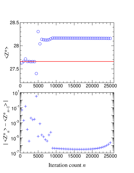
Figure 2: Average charge (upper figure) and its variation from one step to the previous (lower figure) in Kr as computed with conjugate gradient method starting on Saha-Boltzmann populations. The horizontal red line corresponds to the average charge as determined by the stable Gauss algorithm. The electron temperature and density are 1000 eV and $10^{14}\text{ cm}^{-3}$ respectively. The $\varepsilon$ parameter of Eq. (1) is $10^{-13}$.

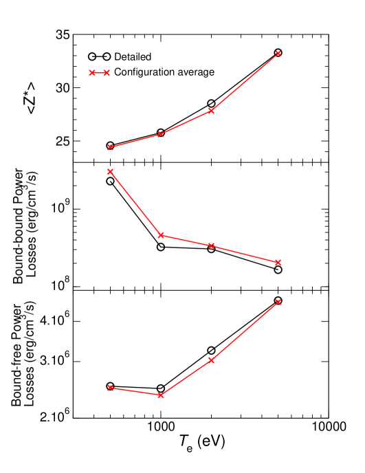
Figure 5: Average charge, radiative bound-bound and bound-free losses for a krypton plasma at $10^{14}\text{ cm}^{-3}$ electronic density as a function of the temperature in eV. Computations are performed using detailed levels and configuration average.

References

- [1] M. Al Rabban, M. Richardson, H. Scott, F. Gilleron, M. Poirier, T. Blenski, Modeling LPP Sources, EUV Sources for Lithography, SPIE Press, Bellingham, Washington USA, 2006, Ch. 10, pp. 299–337.
- [2] K. Nishihara, A. Sasaki, A. Sunahara, T. Nishikawa, EUV Sources for Lithography, SPIE Press, Bellingham, Washington USA, 2006, Ch. 11, pp. 339–370.
- [3] P. Hakel, M. Sherrill, S. Mazevet, J. J. Abdallah, J. Colgan, D. Kilcrease, N. Magee, C. Fontes, H. Zhang, The new Los Alamos opacity code ATOMIC, J. Quant. Spectrosc. Radiat. Transfer 99 (2006) 265–271.
- [4] A. Bar-Shalom, J. Oreg, M. Klapisch, Recent developments in the SCROLL model, J. Quant. Spectrosc. Radiat. Transfer 65 (2000) 43–55.
- [5] J. Bauche, C. Bauche-Arnoult, K. B. Fournier, Model for computing superconfiguration temperatures in nonlocal-thermodynamic-equilibrium hot plasmas, Phys. Rev. E 69 (2004) 026403.
- [6] R. Rodríguez, J. Gil, R. Florido, J. Rubiano, P. Martel, E. Mínguez, Code to calculate optical properties for plasmas in a wide range of densities, J. Phys. IV 133 (2006) 981–984.
- [7] O. Peyrusse, On the superconfiguration approach to model NLTE plasma emission, J. Quant. Spectrosc. Radiat. Transfer 71 (2001) 571–579.
- [8] H. Chung, M. Chen, W. Morgan, Yu. Ralchenko, R. Lee, FLYCHK: generalized population kinetics and spectral model for rapid spectroscopic analysis for all elements, High Energy Density Physics 1 (2005) 3–12.
- [9] H. A. Scott, Cretin–a radiative transfer capability for laboratory plasmas, J. Quant. Spectrosc. Radiat. Transfer 71 (2001) 689–701.
- [10] Yu. V. Ralchenko, Y. Maron, Accelerated recombination due to resonant deexcitation of metastable states, J. Quant. Spectrosc. Radiat. Transfer 71 (2001) 609–621.
- [11] A. Sasaki, T. Kawachi, Kinetics modeling of ni-like multiple charged ions, J. Quant. Spectrosc. Radiat. Transfer 81 (2003) 411–419.
- [12] G. Faussurier, C. Blancard, E. Berthier, Nonlocal thermodynamic equilibrium self-consistent average-atom model for plasma physics, Phys. Rev. E 63 (2001) 026401.
- [13] C. Bowen, A. Decoster, C. J. Fontes, K. B. Fournier, O. Peyrusse, Yu. Ralchenko, Review of the NLTE emissivities code comparison virtual workshop, J. Quant. Spectrosc. Radiat. Transfer 81 (2003) 71–84.
- [14] C. Bowen, R. W. Lee, Yu. Ralchenko, Comparing plasma population kinetics codes: Review of the NLTE-3 kinetics workshop, J. Quant. Spectrosc. Radiat. Transfer 99 (2006) 102–119.
- [15] J. Rubiano, R. Florido, Bowen, R. Lee, Yu. Ralchenko, Review of the 4th NLTE code comparison workshop, High Energy Density Physics 3 (2007) 225–232.
- [16] C. J. Fontes, J. Abdallah, Jr., C. Bowen, R. W. Lee, Yu. Ralchenko, Review of the NLTE-5 kinetics workshop, in this issue.
- [17] M. Poirier, F. de Gaufridy de Dortan, A comparison between detailed and configuration-averaged collisional-radiative codes applied to non-local thermal equilibrium plasmas, J. Appl. Phys. 101 (2007) 063308.
- [18] S. Hansen, K. B. Fournier, C. Bauche-Arnoult, J. Bauche, O. Peyrusse, A comparison of detailed level and superconfiguration models of neon, J. Quant. Spectrosc. Radiat. Transfer 99 (2006) 272–282.
- [19] S. Kaushik, P. L. Hagelstein, The application of conjugate gradient methods to NLTE rate matrix equations, Appl. Phys. B 50 (1990) 303–306.
- [20] W. H. Press, S. A. Teukolsky, W. T. Vetterling, B. P. Flannery, Numerical Recipes: The Art of Scientific Computing, 3rd Edition, Cambridge University Press, Cambridge, UK, 2007.
- [21] M. Poirier, On various validity criteria for the configuration average in collisional-radiative codes, J. Phys. B 41 (2008) 025701.
- [22] K. B. Fournier, M. May, D. Pacella, M. Finkenthal, B. Gregory, W. Goldstein, Calculation of the radiative cooling coefficient for krypton in a low density plasma, Nuclear Fusion 40 (2000) 847–864.
- [23] A. Bar-Shalom, M. Klapisch, J. Oreg, HULLAC, an integrated computer package for atomic processes in plasmas, J. Quant. Spectrosc. Radiat. Transfer 71 (2001) 169–188.
- [24] J. Wesson, Tokamaks, 3rd Edition, Clarendon Press, Oxford, UK, 2004.
- [25] T. Hirai, H. Maier, M. Rubel, P. Mertens, R. Neu, E. Gauthier, J. Likonen, C. Lungu, G. Maddaluno, G. Matthews, R. Mitteau, O. Neubauer, G. Piazza, V.Philipps, B. Riccardi, C. Ruset, I. Uytdenhouwen, R&D on full tungsten divertor and beryllium wall for JET ITER-like wall project, Fus. Eng. Design 82 (2007) 1839 – 1845.
- [26] Yu. Ralchenko, J. N. Tan, J. D. Gillaspy, J. M. Pomeroy, E. Silver, Accurate modeling of benchmark x-ray spectra from highly charged ions of tungsten, Phys. Rev. A 74 (2006) 042514.