Restricted orientation “liquid crystal” in two dimensions:
isotropic–nematic transition or liquid–gas (?)

Abstract

We present Monte Carlo simulation results of the two-dimensional Zwanzig fluid, which consists of hard line segments which may orient either horizontally or vertically. At a certain critical fugacity, we observe a phase transition with a two-dimensional Ising critical point. Above the transition point, the system is in an ordered state, with the majority of particles being either horizontally or vertically aligned. In contrast to previous work, we identify the transition as being of the liquid-gas type, as opposed to isotropic-to-nematic. This interpretation naturally accounts for the observed Ising critical behavior. Furthermore, when the Zwanzig fluid is extended to more allowed particle orientations, we argue that in some cases the symmetry of a $q$-state Potts model with $q>2$ arises. This observation is used to interpret a number of previous results.

1 Introduction

In a seminal paper [1], Onsager demonstrated that infinitely slender rods in three dimensions undergo a first-order isotropic-to-nematic (IN) transition. In the nematic phase, there is long-ranged alignment of the particles, while in the isotropic phase the particle orientations are essentially random. In contrast, in two dimensions, long-ranged nematic order is generally absent. For a certain class of liquid crystal pair potentials, the absence of nematic order can be proved rigorously [2], while simulations using different potentials also indicate its absence in the thermodynamic limit [3, 4]. Of course, these results do not imply that there can be no phase transition in two-dimensional (2D) liquid crystals, but rather that any such transition does not lead to nematic order.

Interestingly, a number of papers have appeared recently [5, 6, 7, 8] in which the IN transition was studied in two dimensions. The transition was shown to belong to the universality class of the 2D Ising model. In accordance with the Ising model, this implies the formation of a finite nematic order parameter above the critical density, which seems to contrast the results of [3, 4], where nematic order was found to vanish in the thermodynamic limit. The results of [5, 6, 7, 8] thus raise a number of questions. First of all, how can we understand the formation of finite nematic order in these 2D systems and, secondly, what is the origin of the Ising critical point? In this work, these questions will be answered.

The absence of nematic order in many two dimensional systems is a consequence of the Mermin-Wagner theorem [9, 10, 11]. As is well known, this theorem applies when the particle orientations are continuous. However, when the orientations become discretized, Mermin-Wagner no longer applies, and the corresponding phase behavior changes dramatically. A famous example of a liquid crystal model with discrete orientations is the Zwanzig model [12], where the particles are treated as rigid rods. The particle positions are continuous, but the molecular axis may only point in mutually perpendicular directions. In two dimensions, this implies a system of line segments, which may either point horizontally or vertically. The interactions are of the excluded volume type, meaning that particles may not overlap with each other. A further approximation is to also make the particle positions discrete, i.e. to restrict the line segments to the sites of a square lattice, and to let each segment occupy $k$ consecutive sites. This is precisely the model studied in [5, 6, 7, 8]. For $k=2$ one recovers the dimer model [13], while for $k\to\infty$ one approaches the 2D Zwanzig model. Provided $k\geq 7$ [8], at some threshold density, one finds a transition to a “nematic” phase, in which most particles point either horizontally (“A particles”) or vertically (“B particles”).

However, is this transition truly an IN transition? In this model, there is symmetry under the exchange of A and B particles. That is, given a valid configuration, i.e. one without overlaps, a new valid configuration can be obtained by replacing each A particle with a B particle and vice-versa. Under this operation, the order parameter $|N_{A}-N_{B}|/(N_{A}+N_{B})$ [5] remains invariant, with $N_{i}$ the number of particles of type $i$. Clearly, a liquid crystal with continuous orientations cannot exhibit this symmetry. The observed symmetry rather resembles the particle-hole symmetry of the lattice gas, or the up-down symmetry in the Ising model. This suggests that the IN transition of [5, 6, 7, 8] is really an unmixing or liquid-gas transition. This also accounts for the observed Ising critical behavior, since it is well known that liquid-gas and unmixing transitions in fluids with short ranged interactions belong to this class.

The interpretation in terms of a liquid-gas transition is also consistent with the original paper by Zwanzig [12]. Here, it was already mentioned that, in two dimensions, a mapping of the Zwanzig model onto a mixture of green and red squares [14] is possible, whereby squares of different color may not overlap. This is, of course, just a variant of the Widom-Rowlinson mixture of spherical particles in two dimensions [15], in which the existence of a liquid-gas transition is not debated. Note that the origin of liquid-gas transitions in these systems stems from depletion. One could envision formally integrating out, say, the “red” species, yielding a one component fluid of “green” species, interacting via an effective short-ranged potential with attractive part [16]. Hence, these systems resemble simple fluids, such as the Lenard-Jones fluid, and are expected to yield similar phase diagrams as a result.

In this Letter, these ideas will be applied to the 2D Zwanzig model using computer simulation. We first specify the 2D Zwanzig model, and describe the simulation method. Next, we show that the transition in this model indeed corresponds to a liquid-gas transition, rather than IN. In particular, we demonstrate that a binodal can be constructed, which terminates at an Ising critical point. We also provide estimates for the line-tension between coexisting domains in the two-phase (ordered) region of the phase diagram. Finally, we present a summary and detailed conclusion, where we emphasize that care must be taken when modeling liquid crystal phase transitions using only a discrete set of orientations.

2 model and simulation method

We consider the 2D Zwanzig model, which consists of infinitesimally thin hard rods of unit length. Since the interactions are hard-core, temperature does not play a role, and factors of $k_{B}T$ are set to unity throughout (with $k_{B}$ the Boltzmann constant and $T$ the temperature). The rods may be aligned horizontally (“$A$ particles”) or vertically (“$B$ particles”). The particle positions are confined to a periodic 2D square of area $V$. Since the rods are infinitesimally thin, there is only a hard-core interaction between $A$ and $B$ particles (which may thus not overlap). Hence, each $A$ particle is surrounded by a depletion zone, which may not contain the centers of any $B$ particles (note that the depletion zone for this model is just the unit square). We consider a grand canonical simulation ensemble, with the respective chemical potentials $\mu$ and $\mu_{B}$, of $A$ and $B$ particles, being the relevant thermodynamic parameters; the actual number of particles in the system is a fluctuating quantity. The aim of the simulations is to measure the distribution $P(N|\mu,\mu_{B})$, defined as the probability to observe a system containing $N$ particles of type $A$, at chemical potentials $\mu$ and $\mu_{B}$.

During the simulations, insertion and removal of particles are performed using a grand canonical cluster move [17, 18]. With equal probability, we attempt to insert an $A$ particle, or we attempt to remove one. When inserting, a single $A$ particle is tentatively placed at a random location in the simulation box. This will generally lead to overlap with some $B$ particles, say $n_{B}$ of them. The overlapping $B$ particles are removed from the box, and the resulting state is accepted with probability

$$A(N\to N+1,N_{B}\to N_{B}-n_{B})=\hskip 56.9055pt$$

$$\begin{cases}0&n_{B}\geq\Delta\\ {\rm min}\left[1,\frac{zV}{\Delta(N+1)}\frac{(n_{B})!}{z_{B}^{n_{B}}}\right]&\text{otherwise},\end{cases}$$

with $\Delta$ a parameter to be specified later, and $N_{B}$ the total number of $B$ particles in the system at the beginning of the move. In the above, we have also introduced the respective fugacities $z=\exp(\mu)$ and $z_{B}=\exp(\mu_{B})$, of $A$ and $B$ particles. During removal, one $A$ particle is picked randomly and deleted, and $n_{B}$ centers of $B$ particles are distributed randomly into the depletion zone of the just deleted $A$ particle, with $n_{B}$ a uniform random number $0\leq n_{B}<\Delta$. If any of the inserted $B$ particles overlap with $A$ particles, the move is rejected, otherwise it is accepted with probability

$$A(N\to N-1,N_{B}\to N_{B}+n_{B})=\hskip 56.9055pt$$

$${\rm min}\left[1,\frac{\Delta N}{zV}\frac{z_{B}^{n_{B}}}{(n_{B})!}\right].$$

The reader may verify that this algorithm fulfills detailed balance [17, 18]. The factorials count the number of ways in which $n_{B}$ particles can be distributed onto the unit square. Note that the thermal wavelength has been set to unity for clarity. The parameter $\Delta$ must be high enough such that the insertion of $A$ particles into a pure phase of $B$ particles is efficient. For the present model, a pure phase of $B$ particles is just an ideal gas, for which density equals fugacity. Hence, the depletion zone contains $z_{B}$ $B$ particles on average, with Poissonian fluctuations. Consequently, $\Delta$ should somewhat exceed this value; we found that $\Delta=z_{B}+\sqrt{z_{B}}+2$ gave good results.

The phase transition in our model is characterized by a free energy functional featuring two minima separated by a barrier. Apart from a minus sign, the free energy is just the logarithm of the distribution $P(N|\mu,\mu_{B})$ that we wish to find, and we define $W(N)\equiv\ln P(N)$. Computer simulations which directly sample the Boltzmann distribution are not efficient then, since these tend to “get stuck” in one of the minima, and rarely cross the barrier. To overcome this problem, we combine the grand canonical cluster move with a biased sampling method called successive umbrella sampling (SUS) [19]. In SUS, $W(N)$ is obtained recursively by splitting the simulation into a number of windows. In the first window, the number of $A$ particles is allowed to fluctuate between 0 and 1, in the second window between 1 and 2, and so forth. There is no restriction on the number of $B$ particles though, and $N_{B}$ fluctuates freely in each window. By simulating the $N$-th window, one immediately obtains the free energy difference

$$\Delta F(N|\mu,\mu_{B})\equiv W(N)-W(N-1)=\ln\left(C_{+}/C_{-}\right),$$ (1)

with $C_{+}$ ($C_{-}$) the number of times that the (unbiased) simulation was in a state with $N$ ($N-1$) particles of type $A$ (irrespective of $N_{B}$). Obviously, the free energy difference depends on $\mu$ and $\mu_{B}$. Once the free energy differences have been measured over a range of windows, $W(N)$ can be constructed via recursion

$$W(0)\equiv 0,\hskip 14.22636ptW(N)=W(N-1)+\Delta F(N).$$ (2)

Using that $P(N)\propto e^{W(N)}$, one trivially converts to the sought-for distribution $P(N|\mu,\mu_{B})$.

An additional ingredient of this work is histogram reweighting, which we use to extrapolate simulation data obtained at $(\mu,\mu_{B})$ to different chemical potentials $(\mu^{\prime},\mu_{B}^{\prime})$. In order to extrapolate in $\mu_{B}$, we also require the distributions $R(N_{B}|N,\mu_{B})$, defined as the probability to observe a system containing $N_{B}$ particles of type $B$, when the number of $A$ particles equals $N$, at chemical potential $\mu_{B}$ (since $R(N_{B}|N,\mu_{B})$ is obtained for fixed $N$, there is no dependence on $\mu$). For example, $R(N_{B}|0,\mu_{B})$ is the distribution in $B$ particles when no $A$ particles are present (this corresponds to an ideal gas at chemical potential $\mu_{B}$, and hence a single Poissonian peak). The expression to extrapolate the free energy difference obtained at $(\mu,\mu_{B})$ to $(\mu^{\prime},\mu_{B}^{\prime})$ then becomes

$$\Delta F(N|\mu^{\prime},\mu_{B}^{\prime})=\hskip 113.81102pt$$

$$\Delta F(N|\mu,\mu_{B})+\mu^{\prime}-\mu+\ln\frac{{\cal Z}(N)}{{\cal Z}(N-1)},$$ (3)

with

$${\cal Z}(N)=\frac{\sum_{N_{B}}R(N_{B}|N,\mu_{B})e^{(\mu_{B}^{\prime}-\mu_{B})N_{B}}}{\sum_{N_{B}}R(N_{B}|N,\mu_{B})}.$$ (4)

Note that ${\cal Z}(N)$ is simply the relative change in the “volume” of $R(N_{B}|N,\mu_{B})$ when extrapolating from $\mu_{B}\to\mu_{B}^{\prime}$. By using Eq.(2), in combination with the recursion relation, it becomes possible to construct $P(N|\mu^{\prime},\mu_{B}^{\prime})$, without actually having to perform a simulation at $\mu^{\prime}$ and $\mu_{B}^{\prime}$.

The quality of Eq.(2) deteriorates when the range in chemical potential over which one extrapolates becomes large. For each system size, we therefore perform a series of $i=1,\ldots,k$ SUS simulations, over a range of chemical potentials $\mu_{i}$ and $\mu_{B,i}$. Due to symmetry, we set $\mu_{i}=\mu_{B,i}$ for convenience, although this is not essential. Using Eq.(2), each one of these simulations yields an estimate of the free energy difference $\Delta F_{i}(N|\mu,\mu_{B})\pm\sigma_{i}$, where $\sigma_{i}$ is an estimate of the statistical error. Next, we weight each estimate with its inverse square error to obtain the best estimate of the free energy difference

$$\Delta F_{\rm best}(N|\mu,\mu_{B})=\frac{\sum_{i=1}^{k}\Delta F_{i}(N|\mu,\mu_{B})/\sigma_{i}^{2}}{\sum_{i=1}^{k}1/\sigma_{i}^{2}},$$ (5)

which is then fed into the recursion relation to construct the best estimate of $P(N|\mu,\mu_{B})$ for some $\mu,\mu_{B}$ of interest. To derive $\sigma_{i}$, we note that statistical errors occur in the counts $C_{+}$ and $C_{-}$, as well as in the histogram entries $R(N_{B}|N,\mu_{B})$. In principle, these errors are Poissonian

$$\sigma[C_{+}]=\sqrt{C_{+}},\hskip 14.22636pt\sigma[C_{-}]=\sqrt{C_{-}},$$

$$\sigma\left[R(N_{B}|N,\mu_{B})\right]=\sqrt{R(N_{B}|N,\mu_{B})},$$

but only if the data are normalized to the number of independent measurements. This requires knowledge of the correlation time $\tau$, which is computationally expensive to obtain, since the acceptance rate of the cluster move, and hence $\tau$, depend sensitively on density, composition, and system size. Instead, we follow a more pragmatic approach, whereby $C_{+}$ and $C_{-}$ are normalized to the number of accepted cluster moves in the window. Similarly, the histogram $R(N_{B}|N,\mu_{B})$ is normalized to the number of cluster moves which resulted in a state with $N$ particles of type $A$ and which involved a change in the number of $B$ particles. With these choices, we assume that the statistical errors become Poissonian, i.e. proportional to square-roots, with a common proportionality constant. Next, a propagation of errors calculation can be applied to Eq.(2) and Eq.(4) to derive $\sigma_{i}$. A final important optimization is to combine the set of histograms $R_{i}(N_{B}|N,\mu_{B,i})$ from the various SUS simulations into one best estimate using the multiple histogram method [20, 21], and to subsequently use this best estimate to calculate ${\cal Z}(N)$ of Eq.(4).

3 Results

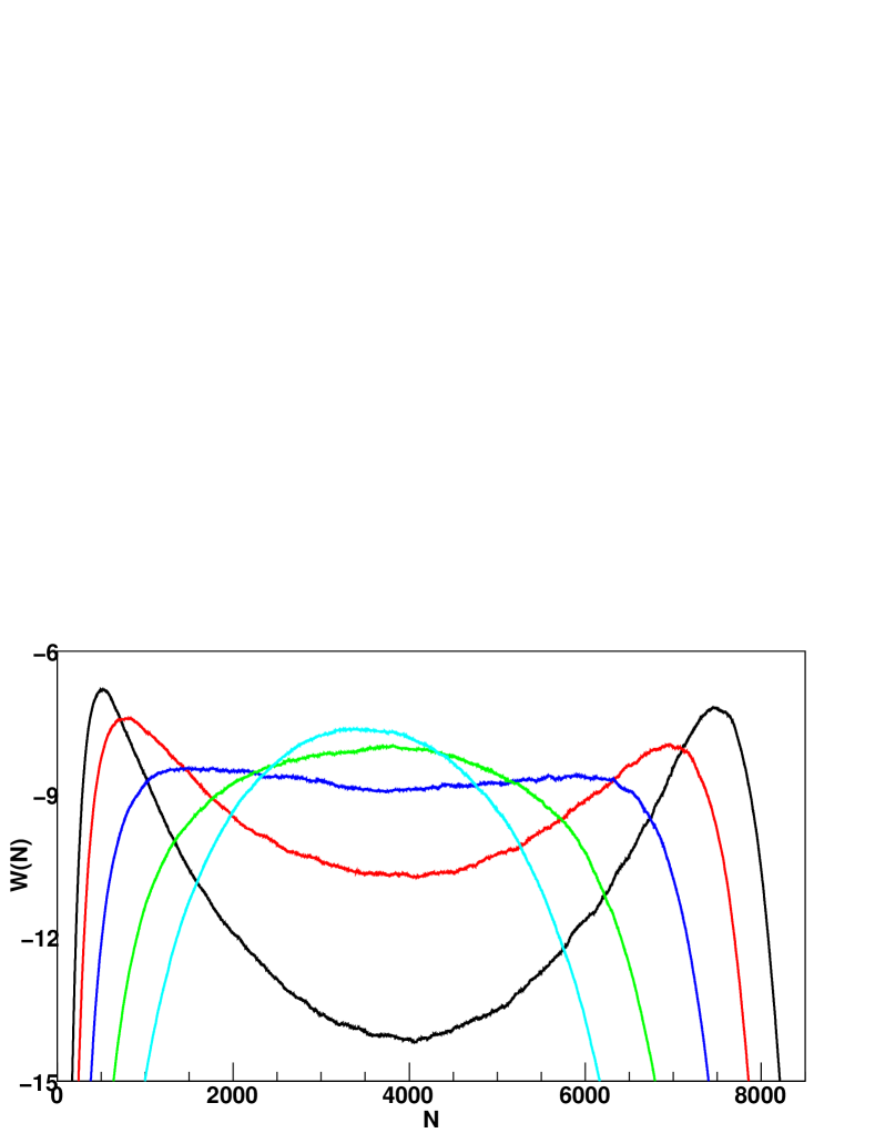
Figure 1: Distributions $W(N)$ obtained in a $40\times 40$ system. The distributions were measured at $z_{B}=5.0,5.1,5.2,5.3,5.4$, and clearly illustrate the formation of the double-peaked structure with increasing $z_{B}$.

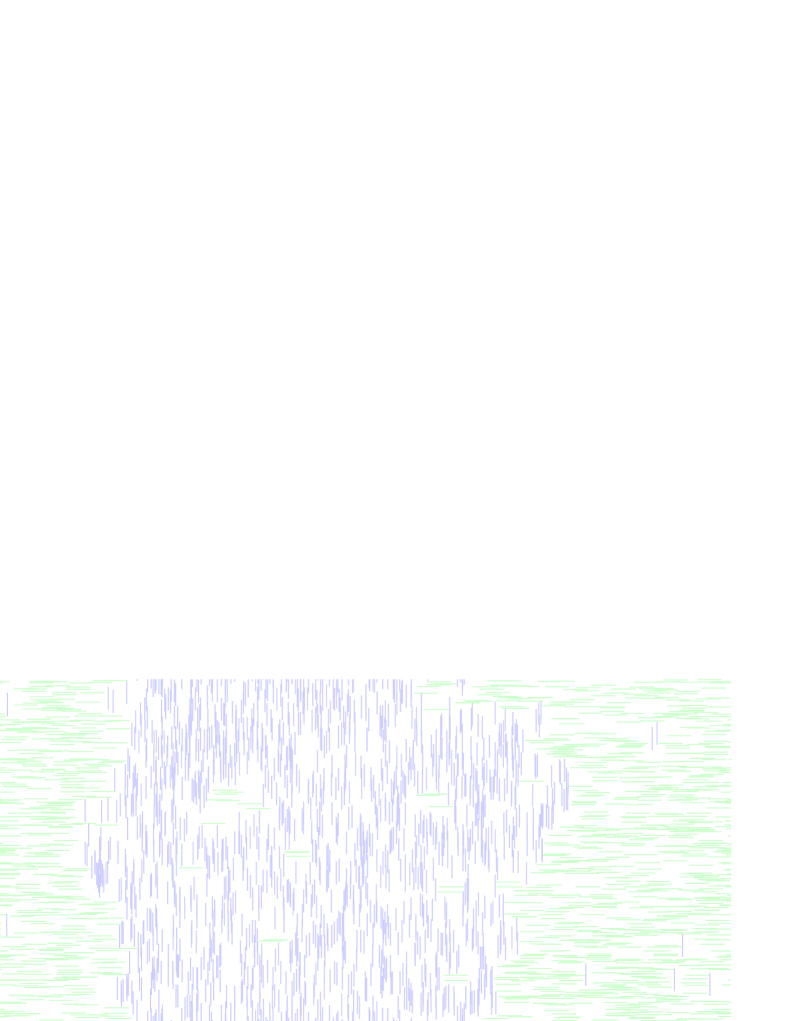
Figure 2: Snapshot of the 2D Zwanzig model at coexistence in a rectangular $L\times D$ simulation box, with $L=30$ and $D=15$, at fugacity $z_{B}=6.0$.

In Fig. 1, we show distributions $W(N)=\ln P(N)$, for a number of fugacities $z_{B}$. For sufficiently large $z_{B}$, the distributions develop two pronounced peaks: one at low density $\rho=N/V$ of $A$ particles, and one at high density. Note that the bimodal structure only shows-up if the fugacity $z$ of the $A$ particles is chosen suitably. For the present model, of course, we may set $z=z_{B}$ due to symmetry, which was adopted throughout this work. For asymmetric fluids, choosing $z$ is less straightforward, and many criteria can, in fact, be defined [22].

The connection to the liquid-gas transition becomes clear if one “identifies” the low-density peak with the gas phase, the high-density peak with the liquid, and $z_{B}$ with inverse temperature. The region between the peaks reflects phase coexistence, whereby both phases appear simultaneously. In simulations, the coexistence can be visualized directly (Fig. 2). Note that a rectangular simulation box is used, and so the interfaces form parallel to the short edge, since this minimizes the total amount of interface (due to periodic boundary conditions, two interfaces are actually present). The corresponding distribution $W(N)$ for the rectangular system is shown in Fig. 3. Note the flat region between the peaks, implying that interactions between the interfaces are absent. Following Binder [23], the height of the barrier $\Delta W$ in Fig. 3 yields the line tension $\sigma_{l}=\Delta W/2D$, with $D$ the short edge of the rectangle. For $z_{B}=6.0$ we obtain $\sigma_{l}\approx 0.47$ (in units of $k_{B}T$ per particle length). As expected, the line tension increases rapidly with increasing $z_{B}$, as manifested by the growing barriers of Fig. 1.

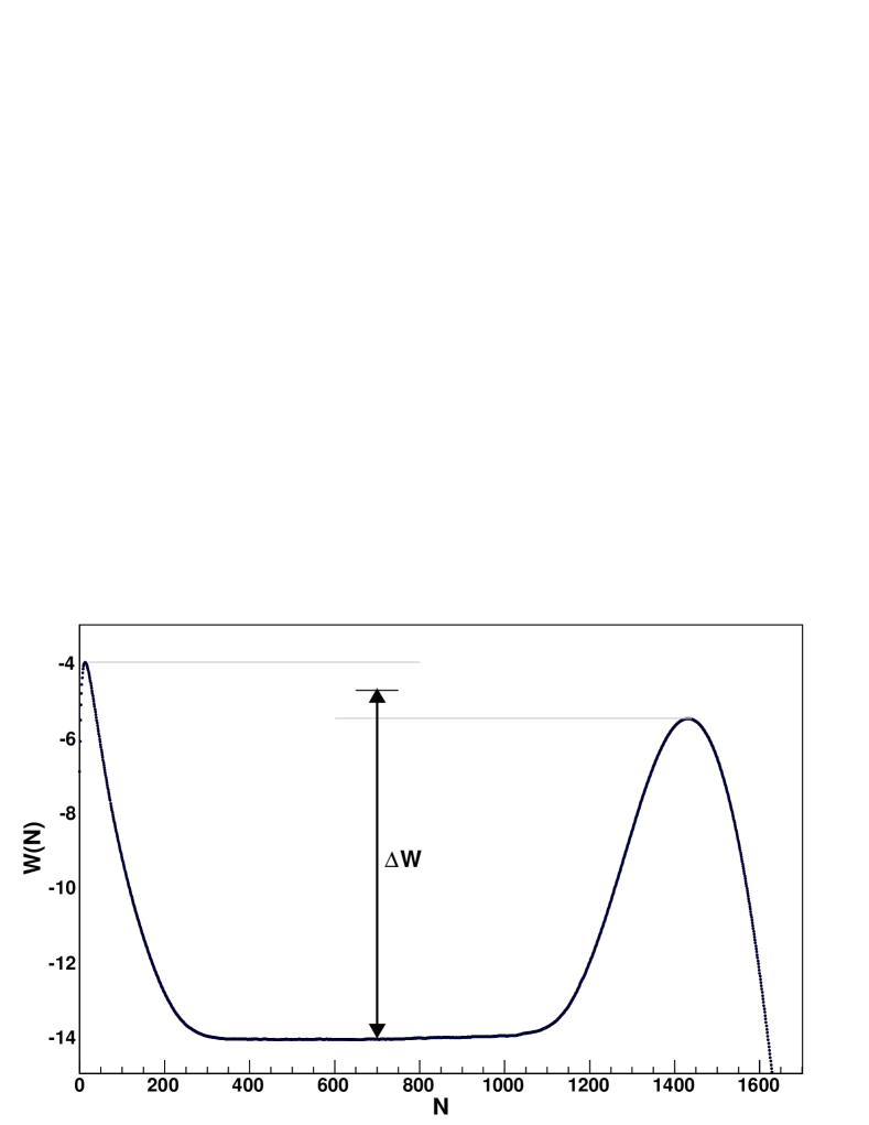
Figure 3: $W(N)$ as obtained in a rectangular $25\times 10$ system at $z_{B}=6.0$. Note the flat region in between the peaks, and also the definition of the barrier $\Delta W$.

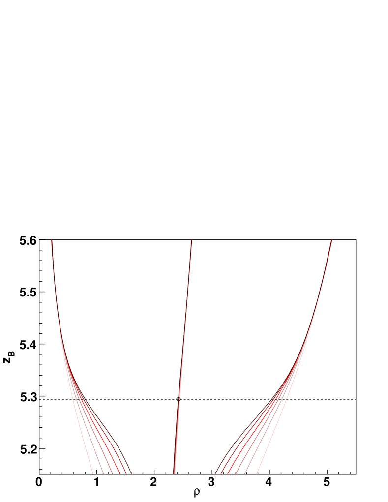
Figure 4: Phase diagram (binodal) of the 2D Zwanzig model for system sizes $L=15,20,\dots,40$ (from outer to inner). The left (right) branches mark the positions of the gas (liquid) peak, the horizontal line is the critical fugacity $z_{B,\rm cr}\approx 5.294$ obtained from Fig. 5(a). Also shown are the diameters (middle curves). The intersection of the diameter with the horizontal line yields the critical point (circle).

Figure 5: Finite size scaling analysis of the susceptibility $\chi_{L}$. (a) Positions of the peak maxima $z_{B,L}$ versus $1/L$. The line is a linear fit from which $z_{B,\rm cr}$ follows. (b) The values $\chi_{L,\rm max}$ at the maxima versus $L$. The curve is a fit to a powerlaw, see details in the text, from which the critical exponent $\gamma$ follows.

In analogy to the liquid-gas transition, we can construct a binodal, by plotting the peak positions in $P(N)$ as a function of $z_{B}$ (Fig. 4). In the thermodynamic limit $L\to\infty$, the gas and liquid branches of the binodal meet at the critical point, while in finite systems they “sway” around it (finite-size rounding [24]). The horizontal line in Fig. 4 marks the thermodynamic limit estimate of the critical fugacity $z_{B,\rm cr}$, taken from Fig. 5. Also shown in Fig. 4 are the “diameters”, defined as the average of the gas and liquid peak positions. In contrast to the binodal, finite size effects in the diameter are much weaker, the reason being that the singularity in the latter is only logarithmic in two dimensional Ising systems [25]. From the intersection of the diameter with the line $z_{B,\rm cr}$ in Fig. 4, we obtain $\rho_{\rm cr}\approx 2.42$ for the critical density of $A$ particles. Due to symmetry, the overall particle density is twice this value.

The critical fugacity $z_{B,\rm cr}$ was obtained from a scaling analysis of the finite-size susceptibility [22]

$$\chi_{L}=\frac{{\langle m^{2}\rangle}-{\langle|m|\rangle}^{2}}{L^{2}},$$ (6)

with $m=N-{\langle N\rangle}$. Following standard arguments [21], $\chi_{L}$ versus $z_{B}$ exhibits a maximum, at position $z_{B,L}$ and with value $\chi_{L,\rm max}$. The peak positions scale with $L$ according to $z_{B,L}-z_{B,\rm cr}\propto L^{-1/\nu}$, with $\nu$ the critical exponent of the correlation length. Using the 2D Ising value $\nu=1$, we observe excellent scaling, see Fig. 5(a), and by fitting we obtain $z_{B,\rm cr}\approx 5.294$. Of course, due to symmetry, the critical fugacity of the $A$ particles is also equal to this value. In addition, the peak maxima are expected to scale as $\chi_{L,\rm max}\propto L^{\gamma/\nu}$, with $\gamma$ the critical exponent of the susceptibility. Indeed, the maxima scale accordingly, see Fig. 5(b), and by fitting we obtain $\gamma\approx 1.76$, in good agreement with the 2D Ising value $\gamma_{2D,I}=7/4$.

4 Discussion

We have shown that the 2D Zwanzig model undergoes a liquid-gas transition at critical fugacity $z_{\rm cr}\approx 5.294$. As expected for systems with short-ranged interactions, the transition belongs to the universality class of the 2D Ising model. Note that the model studied here corresponds to that of hard rods on square lattices, in the limit where the rod length $k\to\infty$. As was shown in [6], the square lattice variant also exhibits a 2D Ising critical point, consistent with our findings. In these and other works [5, 6, 7, 8], the resulting order above $z_{\rm cr}$ is termed nematic, and the corresponding transition at $z_{\rm cr}$ an isotropic-to-nematic transition. In contrast, our work indicates that the transition is just the liquid-gas transition. Therefore, the resulting order should be termed magnetic, since the liquid-gas transition is isomorphic to the formation of a spontaneous magnetization in the Ising model below its critical temperature.

Further evidence in favor of a liquid-gas transition, and against isotropic-to-nematic, is the coexistence between ordered states, see Fig. 2. Note that phase coexistence in the 2D Zwanzig model is possible for all fugacities in the ordered region $z>z_{\rm cr}$ of the phase diagram. The latter is analogous to the coexistence between domains of negative and positive magnetization in the Ising model below its critical temperature. In both cases, the line tension increases as one moves deeper into the ordered region. The corresponding interfaces are therefore order-order interfaces, which (likely) do not exist between nematic phases of liquid crystals, where the particle orientations are continuous [26, 27]. Of course, liquid crystals may exhibit isotropic-nematic coexistence, at a first-order isotropic-to-nematic transition. In that case one has order-disorder interfaces, which survive only at the transition point.

For the 2D Widom-Rowlinson (WR) model consisting of disks, the (single-species) critical density equals $\rho_{\rm cr}\approx 0.78$, while for the critical fugacity $z_{\rm cr}\approx 1.73$ is obtained [16]. These values are significantly below the Zwanzig values reported here, implying a rather weak depletion effect in the latter. This can be made plausible by considering the excluded volume per particle. In a fluid of line segments, unlike segments exclude a volume $l^{2}$, with $l$ being the length. In a mixture of disks, one obtains $\pi l^{2}$, with $l$ being the disk diameter. Hence, the excluded volume per particle is $\pi$ times larger in fluids consisting of disks, and so we expect the transition at a density and fugacity reduced by roughly the same factor. Indeed, inspection of the reported numerical estimates follow this prediction reasonably well (to within 3%).

Our main conclusion is therefore that phase transitions observed in the 2D Zwanzig model and its lattice variants should not be compared to liquid crystal transitions, but instead to transitions observed in simple fluids. This not only includes liquid-gas transitions, but also the possibility of crystallization at high density. Of course, the model considered in the present work cannot crystallize, since the particles are infinitely thin, but the lattice variants considered elsewhere may [5, 6, 7, 8]. Interestingly, these works indeed report evidence of a second transition occurring at high density; whether this transition can be interpreted in terms of (quasi) crystallization [28] could be an interesting topic.

Finally, we discuss the expected trends when the 2D Zwanzig model is extended to a larger set of particle orientations. For hard rods on triangular lattices, the universality class is that of the 2D $3$-state Potts model [6]. We expect the same universality class for an off-lattice fluid of hard line segments, with three allowed orientations $\theta\in\{0,\pi/3,2\pi/3\}$ per segment (with $\theta$ the angle between, say, the segment and the $x$-axes). In the Potts model [29], the nearest-neighbor spin interaction assumes two values: a low (energetically favorable) value when two neighboring spins are in the same state, and a higher value when they are not. For line segments, the analogue is the excluded volume $a_{d}=|\sin\phi|$ between pairs of segments, with $\phi$ the angle between the segments. The reader can verify that for the above set of three orientations, one either has $a_{d}=0$ (when two segments are aligned) or $a_{d}=\sqrt{3}/2$ (when they are not). The excluded volume term thus exhibits the same symmetry as the Potts pair interaction, which naturally accounts for the observed critical behavior on triangular lattices [6]. However, for larger sets of allowed orientations, we expect the analogy to the Potts model to break down. For instance, allowing four orientations $\theta\in\{0,\pi/4,\pi/2,3\pi/4\}$, the excluded volume already assumes three values, in disagreement with Potts symmetry. Note that the analogy to the Potts model may also be useful to interpret results obtained in three dimensions. In this case, the Zwanzig model consists of hard rods of finite width, allowed to point in three mutually perpendicular directions. In terms of symmetry, this corresponds to a three-dimensional $3$-state Potts model, which has a first-order phase transition [30, 31]. The latter is indeed consistent with Zwanzig’s result, where the existence of a first-order transition was also demonstrated [12]. In three dimensions, it should also be possible to realize $4$-state Potts symmetry, by choosing the rod orientations perpendicular to the faces of a regular tetrahedron. For larger sets of orientations, the analogy to the Potts model is again expected to break down. We refer the interested reader to [32, 33] where Zwanzig models with large sets of allowed particle orientations are discussed.

In summary, we have presented simulation results of the 2D Zwanzig model. In agreement with lattice variants of this model, we find a phase transition with critical point belonging to the universality class of the 2D Ising model. The novelty of the present work has been the interpretation of this transition in terms of the liquid-gas transition, as opposed to isotropic-to-nematic. This interpretation accounts naturally for the observed critical behavior, as well as for the observed phase coexistence in the ordered region of the phase diagram. In addition, the excluded volume interaction in fluids of hard line segments with restricted orientations, was shown to resemble in some cases the symmetry of the $q$-state Potts model with $q>2$, thereby elucidating a previous simulation result [6].

- [1] L. Onsager, Ann. N. Y. Acad. Sci. 51, 627 (1949).
- [2] J. P. Straley, Phys. Rev. A 4, 675 (1971).
- [3] D. Frenkel and R. Eppenga, Phys. Rev. A 31, 1776 (1985).
- [4] M. A. Bates and D. Frenkel, J. Chem. Phys. 112, 10034 (2000).
- [5] A. Ghosh and D. Dhar, Europhysics Letters 78, 20003+ (2007).
- [6] M. D. A. Fernandez, D. H. Linares, and R. A. J. Pastor, EPL (Europhysics Letters) 82, 50007+ (2008).
- [7] D. H. Linares, F. Romá, and A. J. Ramirez-Pastor, J. Stat. Mech. 2008, P03013+ (2008).
- [8] M. D. A. Fernandez, D. H. Linares, and R. A. J. Pastor, The Journal of Chemical Physics 128, 214902 (2008).
- [9] N. D. Mermin and H. Wagner, Phys. Rev. Lett. 17, 1133 (1966).
- [10] P. Bruno, Phys. Rev. Lett. 87, 137203 (2001).
- [11] D. Ioffe, S. B. Shlosman, and Y. Velenik, Commun. Math. Phys. 226, 433 (2002).
- [12] R. Zwanzig, The Journal of Chemical Physics 39, 1714 (1963).
- [13] H. N. V. Temperley and M. E. Fisher, Philosophical Magazine 6, 1061 (1961).
- [14] W. G. Hoover and A. G. De Rocco, The Journal of Chemical Physics 36, 3141 (1962).
- [15] B. Widom and J. S. Rowlinson, The Journal of Chemical Physics 52, 1670 (1970).
- [16] G. Johnson, H. Gould, J. Machta, and L. K. Chayes, Physical Review Letters 79, 2612 (1997).
- [17] R. L. C. Vink and J. Horbach, J. Chem. Phys. 121, 3253 (2004).
- [18] R. L. C. Vink, in Computer Simulation Studies in Condensed-Matter Physics XVI, pages 45–60 (Springer, 2006).
- [19] P. Virnau and M. Müller, J. Chem. Phys. 120, 10925 (2004).
- [20] A. M. Ferrenberg and R. H. Swendsen, Phys. Rev. Lett. 63, 1195 (1989).
- [21] M. E. J. Newman and G. T. Barkema, Monte Carlo Methods in Statistical Physics (Clarendon Press, Oxford, 1999).
- [22] G. Orkoulas, M. E. Fisher, and A. Z. Panagiotopoulos, Phys. Rev. E 63, 051507 (2001).
- [23] K. Binder, Phys. Rev. A 25, 1699 (1982).
- [24] K. Binder and D. W. Heermann, Monte Carlo Simulation in Statistical Physics: An Introduction (Springer, Berlin, Germany, 2002).
- [25] R. L. C. Vink and H. H. Wensink, Phys. Rev. E 74, 010102 (2006).
- [26] J. Fröhlich and C.-E. Pfister, Communications in Mathematical Physics 89, 303 (1983).
- [27] S. Shlosman and Y. Vignaud, Communications in Mathematical Physics 276, 827 (2007).
- [28] K. J. Strandburg, Rev. Mod. Phys. 60, 161 (1988).
- [29] F. Y. Wu, Rev. Mod. Phys. 54, 235 (1982).
- [30] H. W. J. Blöte and R. H. Swendsen, Physical Review Letters 43, 799+ (1979).
- [31] M. Schmidt, Zeitschrift für Physik B Condensed Matter 95, 327 (1994).
- [32] J. P. Straley, The Journal of Chemical Physics 57, 3694 (1972).
- [33] K. Shundyak and R. van Roij, Physical Review E 69, 041703+ (2004).