An Effective Compactness Theorem for Coxeter Groups

Abstract.

Through highly non-constructive methods, works by Bestvina, Culler, Feighn, Morgan, Rips, Shalen, and Thurston show that if a finitely presented group does not split over a virtually solvable subgroup, then the space of its discrete and faithful actions on $\mathbb{H}^{n}$, modulo conjugation, is compact for all dimensions. Although this implies that the space of hyperbolic structures of such groups has finite diameter, the known methods do not give an explicit bound. We establish such a bound for Coxeter groups. We find that either the group splits over a virtually solvable subgroup or there is a constant $C$ and a point in $\mathbb{H}^{n}$ that is moved no more than $C$ by any generator. The constant $C$ depends only on the number of generators of the group, and is independent of the relators.

Introduction

The space of discrete and faithful actions of a given group $G$ on $\mathbb{H}^{n}$, up to conjugation, is a deformation space of the group. It is denoted $\mathcal{D}(G,n)$. In the 1980’s, Thurston proved that when a group $G$ is the fundamental group of an orientable, compact, irreducible, acylindrical 3-manifold with boundary, the deformation space $\mathcal{D}(G,3)$ is compact [Thu86]. To prove this result, Thurston analysed sequences of ideal triangulations.

Inspired by Thurston’s work and Culler-Shalen’s work on varieties of three-manifold groups [CS83], Morgan-Shalen reproved Thurston’s compactness theorem using methods from algebraic geometry and geometric topology [MS84] [MS88a] [MS88b]. Morgan then showed that when $G$ is the fundamental group for a compact, orientable, and irreducible 3-manifold, the space $\mathcal{D}(G,n)$ is compact if and only if the group $G$ does not admit a virtually abelian splitting [Mor86]. This result was pushed to include all finitely-presented groups using the Rips Machine by Bestvina-Feighn, who state the following Compactness Theorem as a consequence of the main result of [BF95] concerning actions of trees:

Compactness Theorem for Finitely Presented Groups (Thurston, Morgan-Shalen, Morgan, Rips, Bestvina-Feighn).

If $G$ be a finitely-presented group that is not virtually abelian and does not split over a virtually solvable subgroup, then $\mathcal{D}(G,n)$ is compact.

If a finitely-presented group does not split over a virtually solvable subgroup, then the Compactness Theorem implies that there is a point in $\mathbb{H}^{n}$ that is not moved too far by any generator, for any action by the group. However, the methods in [BF95] and [Mor86] do not give an explicit bound. The technical adjective ineffective describes such non-constructive results. In contrast, if a proof is constructive or yields explicit quantities, then it is termed effective. The main result of this paper gives an estimate for this uniform bound in the case of Coxeter groups, in terms of the displacement function.

Given a finite presentation of a group $G$ with generators $\{g_{i}\}$, and a representation $\rho:G\to\textnormal{Isom}(\mathbb{H}^{n})$, we define the displacement function of the action corresponding to $\rho$ as the “mini-max” function $\inf_{x\in\mathbb{H}^{n}}\{\max_{i}d(g_{i}x,x)\}$.

Effective Compactness Theorem for Coxeter groups.

Let $G$ be a Coxeter group given by a standard presentation with $k$ generators, and suppose that $G$ admits an isometric discrete and faithful action on $\mathbb{H}^{n}$. There exists a function $C_{n}(k)\in O(k^{4})$ so that either $G$ has a virtually solvable special nontrivial splitting or the displacement function is bounded above by $C_{n}(k)$ for every discrete and faithful action of $G$ on $\mathbb{H}^{n}$. (We state the function explicitly in Section 7.)

This result is related to work by Delzant [Del95] and Barnard [Bar07]. Delzant [Del95] proved an effective compactness theorem for faithful representations of groups to Gromov-hyperbolic groups. Barnard [Bar07] proved an effective compactness theorem for surface groups acting on an arbitrary complete geodesic $\delta$-hyperbolic space, which generalizes the Mumford Compactness Theorem to $\delta$-hyperbolic spaces. Both Delzant and Barnard’s results rely on the assumption that the injectivity radius of the group action is bounded from below. (The result in this paper does not use such an assumption.)

Summary

We begin by recalling the definitions and properties related to Coxeter groups that we use. Section 1 reviews special subgroups of Coxeter groups and defines special splittings following Mihalik and Tschantz’s visual decompositions [MT07].

We then discuss the hyperbolic geometry lemmas needed for the result. In Section 2, we calculate an estimate $\Lambda(\epsilon,R)$ for the length of a geodesic segment in $\mathbb{H}^{n}$ that guarantees that the midpoint of the segment is moved at most $\epsilon$ by an involution, if the translation distance for the endpoints is bounded above by a constant $R$. In Section 3, we show that the quasi-convex hull of a finite set $X$ in $\mathbb{H}^{n}$ is quasi-isometric to the Gromov approximating tree for $X$, which is an abstract tree. In Section 4, we construct a projection of the tree to a collection of geodesic segments in $\mathbb{H}^{n}$ spanning the set $X$, called the “shadow” of the Gromov approximating tree. To show that the shadow is quasi-isometric to a Gromov approximating tree of $X$, we use the quasi-isometry from Section 3.

To relate special splittings to the geometry of the action, we describe a combinatorial framework for assigning labels to the vertices of a tree. Section 5 introduces the system by which we label vertices. In Section 6, we use the fixed points of a Coxeter group action to generate a Gromov approximating tree. We apply the labelling system to the Gromov approximating tree to produce splittings of the Coxeter group. Each edge of the tree yields a special splitting.

In Section 7, we combine the above to prove the main result. We show that when an edge of the Gromov approximating tree is sufficiently long, then the splitting produced by an edge is nontrivial and small. Given an action $\rho$, we find a lower bound on the displacement function of $\rho$ that ensures that the associated Gromov tree contains such a sufficiently long edge. To do so, we apply the estimate $\Lambda(\epsilon,R)$ obtained in Section 2 to geodesics contained in the shadow of the approximating tree, setting $\epsilon$ to the Margulis constant for $\mathbb{H}^{n}$.

Acknowledgments

I am grateful for the insight and mentorship of my advisor Misha Kapovich. I am also thankful for helpful conversations and encouragement from Angela Barnhill, Dick Canary, Indira Chatterji, Thomas Delzant, and Jean Lafont.

1. Coxeter groups

1.1. Notation

We begin by laying out conventions that are used in this paper:

$W$	Coxeter group
$S$	generating set for $W$ in a standard presentation
$(W,S)$	Coxeter system
$\Gamma(W,S)$	Coxeter diagram for system $(W,S)$

The terms above are defined in Section 1.2.

1.2. Overview of Coxeter groups

We briefly recall definitions and and properties of Coxeter groups that are used in the remainder of the paper. The most relevant Coxeter group properties for this paper are: (1) the generators in the standard presentations have finite order (see Definition 1.1), and (2) each relator corresponds to a finite subgroup of $W$ (see Remark 1.2). The length of a relator is inconsequential.

Definition 1.1.

A group $W$ is a Coxeter group if it admits a presentation of the form

$$\langle\,{s_{1},\ldots,s_{g}}\mid{(s_{i}s_{j})^{m_{ij}}}\,\rangle.$$

where $m_{ij}\leq\infty$ and

• $m_{ij}=1$ if and only if $i=j$

• $m_{ij}\geq 2$ when $i>j$.

• $m_{ij}=\infty$ if and only if the element $s_{i}s_{j}$ has infinite order.

We call this presentation a standard presentation.

Denote the set of generators $S=\{s_{1},\ldots,s_{g}\}$. We call the pair $(W,S)$ a Coxeter system and $S$ a fundamental set of generators. We say that the rank of a Coxeter system is the cardinality of $S$.

Remark 1.2.

If $(s_{i}s_{j})^{m_{ij}}$ is a relator in a presentation of $W$, then $\langle{s_{i},s_{j}}\rangle$ is a finite dihedral group.

Later in the paper, we may abbreviate Coxeter system as system.

A Coxeter diagram is a graph that encodes the information given by a standard presentation of a Coxeter group. We denote the graph as $\Gamma(W,S)$. Its vertices correspond to the generators bijectively; each vertex is labelled with its corresponding generator. An edge exists between two vertices $s_{i}$ and $s_{j}$ if and only if $m_{ij}$ is finite and $i\neq j$. This edge is labelled with the number $m_{ij}$. Every Coxeter group determines a Coxeter diagram, a graph whose edges are labelled by positive integers, and any such graph determines a Coxeter system.

Figure 1 shows the diagram corresponding to the reflection group about a hyperbolic quadrilateral with angles $\pi/2$, $\pi/3$, $\pi/4$, $\pi/4$. A standard Coxeter presentation for this group is

$$\langle\,{s_{1},s_{2},s_{3},s_{4}}\mid{s_{i}^{2},(s_{1}s_{2})^{2},(s_{2}s_{3})^{4},(s_{3}s_{4})^{3},(s_{4}s_{1})^{4}}\,\rangle.$$

Figure 1. A sample Coxeter diagram.

Note that if a Coxeter diagram $\Gamma(W,S)$ is disconnected, then the Coxeter group can be expressed as a free product of the groups given by the components. For the remainder of the paper, we work only with Coxeter groups whose diagrams are connected. This assumption will be used in Section 6.2.

By abuse of notation, we may use $s_{i}$ to denote the vertex of the Coxeter diagram that is labelled by the generator $s_{i}$ as well as to denote the generator.

Note that the Coxeter diagram convention differs from the Coxeter graph, where edges are drawn if and only if $2<m_{ij}\leq\infty.$ The Coxeter group associated to a disconnected Coxeter graph can be decomposed into a direct product.

Coxeter diagrams are more common in geometric group theory, while Coxeter graphs are more common in Lie theory and combinatorics.

1.3. Special splittings

Definition 1.3.

Given a Coxeter system $(W,S)$, a subgroup $W^{\prime}$ of $W$ is special if it is generated by a subset of $S$. The notation $(W^{\prime},S^{\prime})\subset(W,S)$ indicates that the subgroup $W^{\prime}$ is generated by $S^{\prime}\subset S$.

As a set of vertices, a subset $S^{\prime}$ spans a unique maximal subdiagram $\Gamma^{\prime}=\Gamma(W^{\prime})$ of the Coxeter diagram $\Gamma(W)$ of $(W,S)$. We say that the subdiagram $\Gamma^{\prime}$ is special and call the associated subgroup $W(S^{\prime})=\langle{S^{\prime}}\rangle$.

A Coxeter system $(W^{\prime\prime},S^{\prime\prime})$ is isomorphic to a special subgroup of $(W,S)$ if there is an injection $j:W^{\prime\prime}\hookrightarrow W$ carrying $S^{\prime\prime}$ to a subset of $S$. We call $j$ a special injection.

Recall that when a group can be expressed as the amalgamated product $A*_{C}B$ or HNN-extension $A*_{C}$, we say that the group splits over $C$, and we refer to the amalgamated product or HNN-extension as a splitting. In this paper, we will not need to consider HNN-extensions. We let the injections defining an amalgamated product be denoted $i_{A}:C\hookrightarrow A$ and $i_{B}:C\hookrightarrow B$. A presentation of an amalgamated product is given by

$$A*_{C}B=\left\langle S(A)\cup S(B)\;\;\bigg{|}\;\;R(A)\cup R(B)\cup\bigcup_{s\in S(C)}\{i_{A}(s)=i_{B}(s)\}\right\rangle,$$

where the group $A$ is given by the presentation $\langle\,{S(A)}\mid{R(A)}\,\rangle$, the group $B$ is given by the presentation $\langle\,{S(B)}\mid{R(B)}\,\rangle$, and amalgamation subgroup $C$ is generated by $S(C)$.

Definition 1.4.

A splitting $W=A*_{C}B$ is a special splitting of a Coxeter system $(W,S)$ if the following conditions hold:

• $A$, $B$, and $C$ are special subgroups of $W$.

• The Coxeter diagram $\Gamma(C)$ is a subdiagram of $\Gamma(A)$ and $\Gamma(B)$.

• Let $j_{A}:A\hookrightarrow W$, $j_{B}:B\hookrightarrow W$, $j_{C}:C\hookrightarrow W$ be special injections for $A$, $B$, $C$ into the Coxeter system $(W,S)$. Let $\Gamma_{A}$, $\Gamma_{B}$, and $\Gamma_{C}$ be the subgraphs of $\Gamma(W)$ induced by the images of the special injection maps. Then the amalgamation maps $i_{A}:C\hookrightarrow A$ and $i_{B}:C\hookrightarrow B$ are induced by the inclusions of the subgraph $\Gamma_{C}$ into $\Gamma_{A}$ and $\Gamma_{B}$.

The conditions in Definition 1.4 are Mihalik and Tschantz’s visual axioms for the case of splittings, or graphs of groups with one edge. The visual axioms for graphs of groups decompositions of Coxeter groups were introduced by Mihalik and Tschantz in [MT07], where the authors used special decompositions to show accessibility with respect to 2-ended splittings and to classify maximal FA-subgroups of finitely generated Coxeter groups.

Definition 1.5.

A splitting is trivial if one of the amalgamation maps $i_{A}$ or $i_{B}$ is an isomorphism.

When the amalgamation groups $A$ and $B$ are Coxeter groups, and $C$ is a special subgroup of $A$ and $B$, then the group $A*_{C}B$ is a Coxeter group as well. Its diagram can be obtained by “visually amalgamating” the Coxeter diagrams for $A$ and $B$ (as graphs), in the following manner:

Definition 1.6.

Suppose that $\alpha_{A}:\Gamma_{C}\hookrightarrow\Gamma_{A},\;\alpha_{B}:\Gamma_{C}\hookrightarrow\Gamma_{B}$ are injections of the labelled simplicial graph $\Gamma_{C}$ carrying edges to edges, vertices to vertices, forgetting vertex labels, and such that labels on edges are preserved. Then the labelled graph

$$\Gamma=\Gamma_{A}\cup\Gamma_{B}/\sim,$$

where $x\sim y$ when $x=\alpha_{A}\circ\alpha_{B}^{-1}(y)$ is called the visual amalgamation of the diagrams $\Gamma_{A}$ and $\Gamma_{B}$ over $\Gamma_{C}$. The edges of $\Gamma$ inherit labels from $\Gamma_{A}$ and $\Gamma_{B}$, and the vertices of $\Gamma$ are unlabelled. We write $\Gamma=\Gamma_{A}\cup_{\Gamma_{C}}\Gamma_{B}.$

Given Coxeter systems $(W_{A},S_{A})$, $(W_{B},S_{B})$, $(W_{C},S_{C})$, let $\Gamma_{A}$, $\Gamma_{B}$, $\Gamma_{C}$ be their associated Coxeter diagrams. Suppose that there are special injections from $W_{C}$ to $W_{A}$ and $W_{B}$ given by $j_{A}:(W_{C},S_{C})\hookrightarrow(W_{A},S_{A})$ and $j_{B}:(W_{C},S_{C})\hookrightarrow(W_{B},S_{B})$. Let $L_{A}:S_{A}\to\textnormal{vert}(\Gamma_{A})$ be the bijection sending $s\in S_{A}$ to the vertex in $\Gamma_{A}$ labelled $s$, and similarly for $B$. Let $L_{C}$ be the bijection between $S_{C}$ and vertices of $\Gamma_{C}$. Let $\alpha_{A}$ and $\alpha_{B}$ be defined as in Definition 1.6. Then the following diagram commutes:

Proposition 1.7.

Let $W=W_{A}*_{W_{C}}W_{B}$, where the amalgamation is given by the maps $j_{A}$ and $j_{B}$. Let $(W^{\prime},S^{\prime})$ be the Coxeter system defined by the diagram $\Gamma$. Then $W\cong W^{\prime}$.

Proof.

By inspection of the commutative diagram following Definition 1.6. ∎

Definition 1.8.

Let $S^{\prime}$ be a subset of generators for the system $(W,S)$. Suppose that there are subgroups $W_{A}\subset W$ and $W_{B}\subset W$, and maps $i_{A}:\langle{S^{\prime}}\rangle\hookrightarrow W_{A}$ and $i_{B}:\langle{S^{\prime}}\rangle\hookrightarrow W_{B}$ so that the amalgamated product $W_{A}*_{\langle{S^{\prime}}\rangle}W_{B}\cong(W,S)$ determined by $i_{A}$ and $i_{B}$ is a special splitting. Then we say that the subset $S^{\prime}$ determines a special splitting of $W$.

Example 1.9.

Suppose $(W,S)=\langle\,{s_{1},s_{2},s_{3},s_{4}}\mid{\{s_{i}^{2}\},\{(s_{i}s_{i+1})^{m_{i,i+1}}\}}\,\rangle$ as in Figure 2. The subset $S^{\prime}=\{s_{1},s_{3}\}$ determines the splitting

$$\langle{s_{1},s_{2},s_{3}}\rangle*_{\langle{s_{1},s_{3}}\rangle}\langle{s_{1},s_{3},s_{4}}\rangle.$$

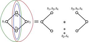
Figure 2. A sample splitting.

Remark 1.10.

A subset does not always determine a unique special splitting, even when $\Gamma$ is connected.

Proposition 1.11.

Suppose that a Coxeter system $(W,S)$ contains a special subgroup $W^{\prime}$ with diagram $\Gamma^{\prime}\subset\Gamma$. Then the subgroup $W^{\prime}$ determines a special splitting of the system $(W,S)$ if and only if the subdiagram $\Gamma^{\prime}$ separates the diagram $\Gamma$.

Proof.

Suppose that $\Gamma^{\prime}$ separates $\Gamma$. Then there exist open nonempty disjoint subsets $\Gamma_{A}^{\prime}$ and $\Gamma_{B}^{\prime}$ of $\Gamma\setminus\Gamma^{\prime}$ that cover $\Gamma\setminus\Gamma^{\prime}$. Let $\Gamma_{A}$ be the maximal subgraph of $\Gamma$ spanned by $\textnormal{vert}(\Gamma^{\prime}\cup\Gamma_{A}^{\prime})$, and set $W_{A}=\langle{\textnormal{vert}(\Gamma_{A})}\rangle$, and similarly for $B$. By Proposition 1.7, the Coxeter system corresponding to the diagram $\Gamma=\Gamma_{A}\cup_{\Gamma^{\prime}}\Gamma_{B}$ is $W_{A}*_{W^{\prime}}W_{B}\cong W$.

Conversely, suppose that $W^{\prime}$ determines a special splitting. Let $W_{A}*_{W^{\prime}}W_{B}$ be a special splitting of $W$. By Proposition 1.7, the Coxeter diagram for $W$ is given by $\Gamma_{A}\cup_{\Gamma^{\prime}}\Gamma_{B}$ with the amalgamation maps induced by the identity inclusion. Hence $\Gamma_{A}\cap\Gamma_{B}=\Gamma^{\prime}$, so $\Gamma^{\prime}$ separates $\Gamma$. ∎

We are ultimately interested in nontrivial special splittings. Recall from Definition 1.5 that trivial splitting occurs when at least one of the groups $W_{A}$ or $W_{B}$ equals $W$. This is the case if and only if $i_{A}:\langle{S_{C}}\rangle\hookrightarrow W_{A}$ or $i_{B}:\langle{S_{C}}\rangle\hookrightarrow W_{B}$ is an isomorphism, so one of $S_{A}$ or $S_{B}$ is the entire set $S$. Thus a trivial splitting occurs when one of the subdiagrams $\Gamma_{A}$ or $\Gamma_{B}$ is the entire diagram $\Gamma$.

2. Bounding the movement of midpoints

The main result of this section is Proposition 2.3, which finds an estimate $\Lambda(\epsilon,R)$ for the length of a geodesic segment $e$ in $\mathbb{H}^{n}$ that guarantees the following: if an isometric involution of $\mathbb{H}^{n}$ moves the endpoints of $e$ at most distance $R$, then the midpoint of $e$ is moved at most $\epsilon$.

Recall that a group is virtually $P$ if it contains a finite index subgroup with property $P$.

Definition 2.1.

A group is small if it is virtually solvable.

Theorem 2.2 (Kazhdan-Margulis Theorem, [KM68]).

There exists a constant $\mu_{n}>0$ (called the Margulis constant for $\mathbb{H}^{n}$) with the following property. Let $x\in\mathbb{H}^{n}$ and $G$ be a discrete subgroup of $\textnormal{Isom}(\mathbb{H}^{n})$ generated by $\{g_{j}\}$ such that

$$d(x,g_{j}(x))\leq\mu_{n}$$

for all $j$. Then the group $G$ is small.

Proposition 2.3.

(See Figure 4.) Set $R\geq 0$. Let $e=[v_{1}v_{2}]$ be a geodesic segment in $\mathbb{H}^{n}$ and let $s$ be an isometric involution of $\mathbb{H}^{n}$. Suppose that they satisfy

$$d(v_{1},s(v_{1})),d(v_{2},s(v_{2}))\leq R.$$

Let $m$ denote the midpoint of $e$. Define $\Lambda(\epsilon,R)$ as

(1) $$\Lambda(\epsilon,R)=\frac{4}{\epsilon}+2R.$$

Then for every $\epsilon>0$, if $d(v_{1},v_{2})\geq\Lambda(\epsilon,R)$, then $d(m,s(m))\leq\epsilon$.

Figure 3. Diagram for Proposition 2.3.

Figure 4. Diagram for Lemma 2.6.

The proof of Proposition 2.3 relies on the convexity of the distance function in hyperbolic space via the propositions that follow.

Here and in future sections, we use $[xy]_{\mathbb{H}}\subset\mathbb{H}^{n}$ to denote the geodesic path between two points $x$ and $y$ in $\mathbb{H}^{n}$. We denote the triangle $[xy]_{\mathbb{H}}\cup[yz]_{\mathbb{H}}\cup[zx]_{\mathbb{H}}$ by $[xyz]_{\mathbb{H}}$ and define a quadrilateral $[xyzw]_{\mathbb{H}}$ similarly. A quadrilateral $[xyzw]_{\mathbb{H}}$ may not necessarily be planar. Where there is no ambiguity, we may suppress subscripts.

Lemma 2.4 (Convexity of the hyperbolic distance function [BH99, II.2, Proposition 2.2]).

. Let $X$ be a geodesic metric space, and $c:[0,1]\to X$ and $c^{\prime}:[0,1]\to X$ be two geodesics parametrized proportionally to arc length. Then for any $t,t^{\prime}\in[0,1]$, the maps $c$ and $c^{\prime}$ satisfy the inequality

$$d(c(t),c^{\prime}(t))\leq(1-t)d(c(0),c^{\prime}(0))+td(c(1),c^{\prime}(1)).$$

The following is an immediate consequence of Lemma 2.4.

Corollary 2.5.

Define $c$ and $c^{\prime}$ as in Lemma 2.4, let $I$ denote the interval $[0,1]$, and let $C^{\prime}=c^{\prime}(I)$. Suppose $d(c(0),c^{\prime}(0)),d(c(1),c^{\prime}(1))\leq r$. Then $d(c(t),C^{\prime})\leq r$ for all $t\in I$.

To obtain the estimate in Proposition 2.3, we use the function

$$h(x)=\sinh^{-1}\left(\frac{1}{\sinh(x)}\right),$$

where $x\in{\mathbb{R}}$ is strictly positive.

Lemma 2.6 ([Kap00, Lemma 3.5, pp. 34-35]).

(See Figure 4.) Let $[xyvw]$ be a quadrilateral in $\mathbb{H}^{n}$ with angles $\angle wxy=\frac{\pi}{2}$, $\angle xyv=\frac{\pi}{2}$, $\angle xwv\geq\frac{\pi}{2}$. Then

$$d(x,w)\leq h(d(x,y)).$$

Corollary 2.7.

Fix $\epsilon>0,R\geq 0$. Let $[xyvw]$ be defined as in Lemma 2.6. Suppose that

$$d(x,w),d(y,v)\leq\frac{R}{2}\textrm{ and }d(v,w)\geq h^{-1}\left(\frac{\epsilon}{2}\right)+R.$$

Then $d(x,w)\leq\frac{\epsilon}{2}$.

Proof of Lemma 2.7.

We first note that $h$ is decreasing. Let $g=h^{-1}(\frac{\epsilon}{2})+R$. Since $d(v,w)\geq g$, we have

$$d(x,y)\geq g-(d(x,w)+d(y,v))\geq g-R$$

and $h(d(x,y))\leq h(g-R)$. We conclude that

$$d(x,w)\leq h(d(x,y))\leq h(g-R)=h\left(h^{-1}\left(\frac{\epsilon}{2}\right)+R-R\right)=\frac{\epsilon}{2}.$$

∎

Proof of Proposition 2.3..

We show that a lower bound of $\Lambda(\epsilon,R)$ on the length of an edge $e$ guarantees an upper bound on the movement of the midpoint $m$ of $e$.

Let $F_{s}$ denote the fixed-point set of the involution $s$. Let $x_{i}$ denote the orthogonal projection of $v_{i}$ to the fixed-point set $F_{s}$. Let $P:e\to[x_{1}x_{2}]$ denote the orthogonal projection from $e$ to the geodesic segment $[x_{1}x_{2}]$, and $m$ be the midpoint of $e$. Then $d(m,P(m))\leq d(v_{i},x_{i})\leq\frac{R}{2}$ by Corollary 2.5.

Suppose that $x_{1}$ and $x_{2}$ are distinct points. Set $x=P(m)$. Either $\angle xmv_{2}\geq\frac{\pi}{2}$ or $\angle xmv_{1}\geq\frac{\pi}{2}$, since they are complementary angles. Without loss of generality, assume that $\angle xmv_{2}\geq\frac{\pi}{2}.$ Then $\angle xs(m)s(v_{2})\geq\frac{\pi}{2}$, and the quadrilaterals $[xx_{2}v_{2}m],[xx_{2}s(v_{2})s(m)]$ satisfy the conditions of Lemma 2.6.

Let $g=h^{-1}(\frac{\epsilon}{2})+R$ as in Corollary 2.7. We assume that the length of $e=[v_{1}v_{2}]$ is at least $2g$, so $d(m,v_{2})=d(s(m),s(v_{2}))\geq g$. Lemma 2.7 shows that $d(x,m)=d(x,s(m))\leq\frac{\epsilon}{2}$. We conclude that

$$d(m,s(m))\leq d(x,m)+d(x,s(m))\leq\epsilon.$$

The case when $x_{1}$ and $x_{2}$ coincide follows by continuity.

We have shown that when the length of $e$ is at least

$$2h^{-1}\left(\frac{\epsilon}{2}\right)+2R,$$

the midpoint of $e$ is moved no more than $\epsilon$.

To complete the proof of the proposition, note that $h^{-1}(x)\leq\frac{1}{x}$. Hence it is sufficient to take the length of the edge $e$ to be at least $\frac{4}{\epsilon}+2R$ as desired. ∎

3. The quasi-convex hull is approximately a tree

Here, we show that the “quasi-convex hull” of a finite subset of $\mathbb{H}^{n}$ is quasi-isometric to the Gromov approximating tree for that subset.

Suppose $X$ is a finite subset of $\mathbb{H}^{n}$. We define its quasi-convex hull $Q(X)$ as the union of geodesic segments between pairs of points of $X$:

$$Q(X)=\bigcup_{x,y\in X}[xy]\subset\mathbb{H}^{n}.$$

We refer to the segments comprising $Q(X)$ as edges of $Q(X)$.

Definition 3.1.

Recall that two spaces $X$ and $Y$ are $(L,A)$-quasi-isometric if, for a given $L>0,A\geq 0$, there is map $f:X\to Y$ such that the following are true:

1. The map $f$ satisfies

   $$-A+\frac{1}{L}d_{X}(x_{1},x_{2})\leq d_{Y}(f(x_{1}),f(x_{2}))\leq Ld_{X}(x_{1},x_{2})+A$$

   for all $x_{1},x_{2}\in X$.

2. There is a map $\overline{f}:Y\to X$ such that

   $$-A+\frac{1}{L}d_{Y}(y_{1},y_{2})\leq d_{X}(\overline{f}(y_{1}),\overline{f}(y_{2}))\leq Ld_{Y}(y_{1},y_{2})+A$$

   for all $y_{1},y_{2}\in Y$.

3. The maps $\overline{f}$ and $f$ satisfy $d_{X}(x,\overline{f}{f}(x))\leq A$ and $d_{Y}(y,f\overline{f}(y))\leq A$.

If there is such an $f$, we call it an $(L,A)$-quasi-isometry. We say a map $f:X\to Y$ is a quasi-isometric embedding if it satisfies Property 1, but there is not necessarily a map $\overline{f}:Y\to X$ that satisfies Properties 2 and 3.

The main result of this section is:

Proposition 3.2.

For any finite set $X\subset\mathbb{H}^{n}$, there is a finite metric tree $T$ which is $(1,A)$-quasi-isometric to $Q(X)$. We may take $A=(20c+12)\ln 3$ for any $c>0$ such that $|X|\leq 2^{c}+2$. Thus $A$ depends only on the cardinality of $X$. (We build the quasi-isometry $P:Q(X)\to T$ in Lemma 3.11.)

The proof of Proposition 3.2 uses the quasi-isometry of a hyperbolic triangle and its comparison tripod (Definition 3.3). We construct the quasi-isometry by first considering the union of maps from individual triangles in $Q(X)$ to tripods in $T$. The union forms a relation, and we refine the relation into the map $P$. We take $T$ to be the Gromov approximating tree (see Definition 3.6).

Definition 3.3.

Let $x_{1},x_{2},x_{3}\in\mathbb{H}^{n}$, and let $\Delta$ denote the triangle $[x_{1}x_{2}x_{3}]$. The unique tripod $\tau_{\Delta}$ with endpoints $a_{1},a_{2},a_{3}$ such that $d_{\mathbb{H}}(x_{i},x_{j})=d_{T}(a_{i},a_{j})$ for all $i,j$ called the comparison tripod of $\Delta$.

Let $\chi_{\Delta}$ be the unique map sending $x_{i}\in X$ to $a_{i}\in\tau_{\Delta}$ for each $i$ and which restricts to an isometry along each edge $[x_{i}x_{j}]\in X$.

Definition 3.4.

Fix $\delta\geq 0$. We say that $\Delta$ is $\delta$-thin if the preimage $y,z\in\chi_{\Delta}^{-1}(x)$ satisfies $d_{X}(y,z)\leq\delta$ for all $x\in X$.

Proposition 3.5 ([CDP90, 4.3]).

All triangles in real hyperbolic $n$-space $\mathbb{H}^{n}$ are delta-hyperbolic for $\delta=\ln{3}$.

Hence we say that $\mathbb{H}^{n}$ is $\delta$-hyperbolic for $\delta=\ln 3$.

Definition 3.6.

Let $X$ be a finite subset of $\mathbb{H}^{n}$ with cardinality $|X|\leq 2^{c}+2$ for $c>0$. We say that a pair $(T,p:X\to T)$ is a Gromov approximating tree if $T$ is a finite metric tree and $p:X\to T$ has the following properties:

1. The map $p:X\to T$ sends points in $X$ to vertices of $T$, and

   $$\partial T\subset p(X),$$

   where $\partial T$ denotes the leaves of $T$ (the valence-one vertices).

2. The distance between pairs of points is quasi-preserved and $p$ does not increase distance:

   $$d_{\mathbb{H}}(x_{1},x_{2})-2c\delta\leq d_{T}(p(x_{1}),p(x_{2}))$$

   for all $x_{1},x_{2}\in X$.

We sometimes abbreviate Gromov approximating tree to approximating tree.

Theorem 3.7 ([GD90, Section 2.1]).

Let $X$ be a finite subset of $\mathbb{H}^{n}$ and cardinality $|X|\leq 2^{c}+2$ for $c>0$. Then there exists a pair $(T,p)$ with the properties described in Definition 3.6.

Remark 3.8.

Gromov’s construction applies to finite $\delta$-hyperbolic spaces and finite sets of rays in $\delta$-hyperbolic spaces.

3.1. Triangles in $Q(X)$

Let $X$ be a finite subset of $\mathbb{H}^{n}$ with cardinality $|X|\leq 2^{c}+2$ for $c>0$, and let $(T,p)$ be a Gromov approximating tree for $X$. Such a tree always exists by Theorem 3.7. We show below that triangles in $Q(X)$ are uniformly quasi-isometric to triangles in $T$ by extending $p:X\to T$ to triangles in $Q(X)$.

Let $[xy]_{T}$ denote the geodesic segment between two points $x,y$ in a tree $T$, and Let $[xyz]_{T}$ denote the tripod in $T$ with leaves $x$, $y$, $z$. We suppress subscripts where there is no ambiguity.

Given $x_{1},x_{2},x_{3}\in X$, let $\Delta$ be the triangle $[x_{1}x_{2}x_{3}]\subset\mathbb{H}^{n}$. Let

$$T_{\Delta}=[p(x_{1})p(x_{2})p(x_{3})]\subset T$$

be the tripod in $T$ with leaves $p(x_{1})$, $p(x_{2})$, $p(x_{3})$. Let

$$o=[p(x_{1})p(x_{2})]\cap[p(x_{2})p(x_{3})]\cap[p(x_{3})p(x_{1})]$$

be the branch point of $T_{\Delta}$. Let $\tau_{\Delta}=[a_{1}a_{2}a_{3}]$ be the comparison tripod (Definition 3.3) of $\Delta$, and let $o_{\tau}=[a_{1}a_{2}]\cap[a_{2}a_{3}]\cap[a_{3}a_{1}]$ be the branch point of $\tau_{\Delta}$. Defining $\chi_{\Delta}:\Delta\to\tau_{\Delta}$ as in Definition 3.3, we call the points in $\chi_{\Delta}^{-1}(o_{\tau})$ the internal points. Note that there is one internal point for each side $[x_{i}x_{j}]$. We label them $o_{12},o_{23},o_{13}$, where $o_{ij}$ is contained in the side $[x_{i}x_{j}]$.

We extend $p|_{\{x_{1},x_{2},x_{3}\}}$ to the unique map $p_{\Delta}:\Delta\to T_{\Delta}$ that

1. sends $x_{i}$ to $p(x_{i})$ for each $i$

2. sends the point $o_{ij}$ to $o$ for each $i,j$

3. maps the segment $[x_{i}o_{ij}]\subset\Delta$ to the segment $[p(x_{i})o]\subset T_{\Delta}$ as a dilation:

   $$d_{T}(p(x_{i}),p_{\Delta}(x))=\frac{d_{T}(p(x_{i}),o)}{d_{\mathbb{H}}(x_{i},o_{ij})}\cdot d(x_{i},x).$$

Proposition 3.9.

The map $p_{\Delta}:\Delta\to T_{\Delta}$ is a $(1,4c\delta+2\delta)$-quasi-isometry, where $\Delta$ is given the subspace metric from $\Delta\subset\mathbb{H}^{n}$.

Proof.

The map $p_{\Delta}$ restricts to a $(1,4c\delta)$-quasi-isometric embedding along an edge $[x_{i}x_{j}]$ in $\Delta$. To show this, we express the distance $d(p(x_{i}),o)$ as

$$d_{T}(p(x_{i}),o)=\frac{1}{2}(d_{T}(p(x_{i}),p(x_{i+1}))+d_{T}(p(x_{i}),p(x_{i-1}))-d_{T}(p(x_{i+1}),p(x_{i-1}))),$$

and combine this with the equations

$$d_{\mathbb{H}}(x_{i},o_{ij})=\frac{1}{2}(d_{\mathbb{H}}(x_{i},x_{i+1})+d_{\mathbb{H}}(x_{i},x_{i-1})-d_{\mathbb{H}}(x_{i+1},x_{i-1}))$$

and

$$d(x_{i},x_{j})-2c\delta\leq d(p(x_{i}),p(x_{j}))\leq d(x_{i},x_{j}).$$

To complete the proof, we consider any $x,y\in\Delta$. In a $\delta$-thin triangle, it is always possible to find $x^{\prime}\in\Delta$ and $y\in\Delta$ so that $x^{\prime}$, $y^{\prime}$ lie along a common side and $d_{\mathbb{H}}(x,x^{\prime})\leq\delta$ and $d_{\mathbb{H}}(y,y^{\prime})\leq\delta$. Hence the map $p_{\Delta}$ is a $(1,4c\delta+2\delta)$-quasi-isometric embedding. Since $p_{\Delta}$ is surjective, it is a quasi-isometry. ∎

3.2. Constructing the quasi-isometry between $Q(X)$ and $T$

To construct the map needed for Proposition 3.2, we use the triangle maps constructed in Section 3.1 to build a relation $P^{\prime}:Q(X)\to T$, and then refine the relation into the desired map.

We define the relation

$$P^{\prime}:Q(X)\to T$$

as follows: given $x\in Q(X)$, the image of $x$ is the set

$$\{p_{\Delta}(x)\in T\mid x\in\Delta\subset Q(X)\}$$

where $p_{\Delta}$ is defined as in Section 3.1. Note that for each $x\in X$, the point $p(x)$ is contained in the image set $P^{\prime}(x)$.

Proposition 3.10.

The relation $P^{\prime}:Q(X)\to T$ satisfies the following three properties:

1. There exists a constant $A^{\prime}$ that uniformly bounds the diameter of $P^{\prime}(x)$ for all $x$.

2. There exists $A$ so that for each pair of points $x_{1},x_{2}\in Q(X)$, we can find $y_{1}\in P^{\prime}(x_{1})$ and $y_{2}\in P^{\prime}(x_{2})$ so that

   $$d(x_{1},x_{2})-A\leq d(y_{1},y_{2})\leq d(x_{1},x_{2})+A.$$

   We may take $A=4c\delta+4\delta$ and $A^{\prime}=8c\delta+4\delta$, so $A$ and $A^{\prime}$ depend only on the cardinality of $X$.

3. The relation $P^{\prime}$ is surjective.

If we can show Proposition 3.10, when we can use the following to complete the proof of Proposition 3.2.

Lemma 3.11.

Let $e$ be an edge of $Q(X)$. Suppose a relation $P^{\prime}:Q(X)\to T$ satisfies the conditions of Proposition 3.10. Then there is a quasi-isometry $P:Q(X)\to T$ so that $P(x)\in P^{\prime}(x)$ for all $x$, the vertices of $T$ are contained in the image of $P$, and $P$ is continuous on $e$.

Proof of Lemma 3.11.

We construct a map $P$, then use the assumed conditions of Proposition 3.10 to show that it satisfies the desired quasi-isometric inequalities.

First note that by construction of $p_{\Delta}$, when $x\in X$, we have $P^{\prime}(x)=p(x)$ (see Section 3.1). So, to construct $P$ from $P^{\prime}$, we pick images for points along edges $[x_{1}x_{2}]\subset Q(X)$, where $x_{1},x_{2}\in X$. Let the vertices of $X$ be $\{x_{1},\dots,x_{k}\}$. Since $X$ is a finite set, there are finitely many edges in $Q(X)$; we order the edges $e_{1},e_{2},e_{3}$, …, etc. Without loss of generality, suppose that $e=e_{1}$ and $x_{1}$ is a boundary vertex of $e_{1}$. We may choose the edges so that $e_{i}=[x_{1}x_{i}]$ for $2\leq i\leq k$.

For each edge $e_{i}$ in $Q(X)$, we pick a triangle $\Delta_{i}$ containing $e_{i}$. Then, for each point $x\in e_{i}\setminus\{e_{1}\cup\dots\cup e_{i-1}\}$, we set $P(x)=p_{\Delta_{i}}(x)$. One can check that the image of the map $P:Q(X)\to T$ thus defined contains all vertices of $T$. By construction, $P$ is continuous on $e$.

To show that $P$ is a quasi-isometry, let $x_{1},x_{2}\in Q(X)$. Combining Property 1 and Property 2 of Proposition 3.10, we have

$$d(x_{1},x_{2})-(A+2A^{\prime})\leq d(P(x_{1}),P(x_{2}))\leq d(x_{1},x_{2})+(A+2A^{\prime}).$$

Hence $P$ is a $(1,A+2A^{\prime})$-quasi-isometric embedding. Property 3 of Proposition 3.10 allows us to construct a quasi-inverse map; to show that the quasi-inverse inequalities are satisfied, we use Properties 1 and 2 of 3.10. ∎

Proof of Proposition 3.10.

To show Property (1), let $x\in Q(X)$. Let $\Delta_{1},\Delta_{2}\subset Q(X)$ be two triangles containing $x$, and suppose that $[x_{1}x_{2}]\subset\Delta_{1},\Delta_{2}$ is the edge of $Q(X)$ containing $x$. By Proposition 3.9,

$$d_{\mathbb{H}}(x,x_{1})-4c\delta-2\delta\leq d_{T}(p_{\Delta_{j}}(x),x_{1})\leq d_{\mathbb{H}}(x,x_{1})+4c\delta+2\delta.$$

Since $p_{\Delta_{1}}(x)$ and $p_{\Delta_{2}}(x)$ lie along the geodesic $[p(x_{1})p(x_{2})]$, it follows that

$$d(p_{\Delta_{1}}(x),p_{\Delta_{2}}(x))\leq 8c\delta+4\delta.$$

Hence we may take $A^{\prime}=8c\delta+4\delta$.

To show Property (2), let $x_{1},x_{2}\in Q(X)$. If $x_{1}$ and $x_{2}$ lie along edges that share a boundary vertex $x\in X$, then the points $x_{1}$ and $x_{2}$ lie in a triangle $\Delta\subset Q(X)$. In this case, Property (2) follows from Proposition 3.9. If $x_{1}$ and $x_{2}$ lie on disjoint edges in $Q(X)$, then they lie on opposite sides of a quadrilateral in $Q(X)$. In this case, it is possible to find two points $x_{1}^{\prime}$ and $x_{2}^{\prime}$ in a common triangle so that $d_{\mathbb{H}}(x_{i},x_{i}^{\prime})\leq\delta$. Let $\Delta^{\prime}$ be a triangle containing $x_{1}^{\prime}$ and $x_{2}^{\prime}$. Then

$$d(x_{1},x_{2})-4c\delta-4\delta\leq d(p_{\Delta^{\prime}}(x_{1}),p_{\Delta^{\prime}}(x_{2}))\leq d(x_{1},x_{2})+4c\delta+4\delta.$$

To show Property (3), let $x_{1},x_{2}\in X$ and $\Delta\subset Q(X)$ be a triangle in $Q(X)$ containing $[x_{1}x_{2}]$. Then $P^{\prime}([x_{1}x_{2}])$ is the geodesic segment $[p(x_{1})p(x_{2})]_{T}$ of $T$. Since $p(X)$ contains all the leaves of $T$, the image $P^{\prime}(Q(X))$ covers all geodesic segments between leaves of $T$. Hence $P^{\prime}$ is surjective. ∎

Proof of Proposition 3.2.

Let $P:Q(X)\to T$ be the map constructed in Lemma 3.11. Then $P$ is an extension of $p$. It follows from Proposition 3.10 and Lemma 3.11 that $P$ is a $(1,20c\delta+12\delta)$-quasi-isometry between $Q(X)$ and $P(Q(X))$. ∎

What we have shown can be summarized as:

Proposition 3.12.

Let $e$ be an edge in $Q(X)$. Then one can find a map $P_{e}:Q(X)\to T$ that is continuous on $e$, and with the property that given $x\in Q(X)$, there is a triangle $\Delta_{x}\subset Q(X)$ where $x\in\Delta_{x}$ and $P_{e}(x)=p_{\Delta_{x}}(x)$. The map $P_{e}$ is an extension of $p$, all vertices of $T$ are contained in the image of $P_{e}$, and $P_{e}$ is a $(1,20c\delta+12\delta)$-quasi-isometry between $Q(X)$ and $T$.

4. The shadow of an approximating tree in $\mathbb{H}^{n}$

The purpose of this section is to define a projection of $T$ into $\mathbb{H}^{n}$, called the “shadow” $T_{\textnormal{sh}}$ of $T$. The shadow is a collection of geodesic segments in $\mathbb{H}^{n}$, and contains $X$.

To set up the definition of the shadow, we define a subset $\overline{X}\subset Q(X)$ as follows: let $V(T)$ denote the vertices of $T$, and let $P:Q(X)\to T$ be a map satisfying the conditions of Proposition 3.12. Then, given $y\in V(T)$, we assign to $y$ a point $x\in Q(X)$ so that $P(x)=y$, with the requirement that if $y\in P(X)$, then the chosen $x$ is an element of $X$. It is always possible to arrange the assignment so that no two points in $V(T)$ are assigned to the same $x$. This follows by construction of the map $P$ and the definition of the Gromov approximating tree. Denote the set of points chosen as $\overline{X}$. The assignment gives a bijection, which we denote as $q_{V}:V(T)\to\overline{X}$. We extend $q_{V}$ to a map $q$, which will allow us to define the “shadow” of $T$.

Proposition 4.1.

Let $q:T\to\mathbb{H}^{n}$ be the extension of $q_{V}:V(T)\to\overline{X}$ which is the unique map sending the edge $[y_{1}y_{2}]\subset T$ to $[q_{V}(y_{1})q_{V}(y_{2})]\subset\mathbb{H}^{n}$ via dilation: given $y\in[y_{1}y_{2}]$, we have

$$d_{\mathbb{H}}(q_{V}(y_{1}),q_{V}(y))=\frac{d_{\mathbb{H}}(q_{V}(y_{1}),q_{V}(y_{2}))}{d_{T}(y_{1},y_{2})}\cdot d_{T}(y_{1},y).$$

Along each edge in $T$, the map $q$ restricts to a $(1,20c\delta+12\delta)$-quasi-isometry.

Proof.

If $y_{1},y_{2}$ are vertices of $T$, then $P(q_{V}(y_{i}))=y_{i}$, for $i=1,2$. Hence we may apply Proposition 3.12 to the map $P:Q(X)\to T$ restricted to the points $y_{1}$ and $y_{2}$, yielding the desired quasi-isometric inequality. ∎

Remark 4.2.

The map $q$ is in fact a $(1,|X|(20c\delta+12\delta))$-quasi-isometry between $T$ and $q(T)$.

Definition 4.3.

We call a point $x=q(y)\in q(T)$ the shadow of $y\in T$.

To define the “shadow” of the tree $T$, we first observe that the image $q(T)$ contains the set $\overline{X}$. Recall the map $p:X\to T$ (Definition 3.6). When $p$ is not injective, then $\overline{X}$ does not contain the original set $X$ generating the Gromov approximating tree. However, if $x\in X\setminus\overline{X}$, there is a unique element $z$ of $\overline{X}$ such that $p(x)=p(z)$.

For ease of exposition in later sections, we define the shadow of $T$ to be a connected union of geodesic segments in $\mathbb{H}^{n}$ containing $q(T)$ and $X$.

Definition 4.4.

We define the shadow of $T$, denoted $T_{\textnormal{sh}}$, as the union of the image $q(T)$ and segments $[xz]\subset\mathbb{H}^{n}$ chosen as follows: if $x\in X$ is not an element of $\overline{X}$, then the segment $[xz]$ is included in $T_{\textnormal{sh}}$, where $z$ is the unique element of $\overline{X}$ such that $p(x)=p(z)$.

If $x_{1}$ and $x_{2}$ are points in $T_{\textnormal{sh}}$, we define $d_{\textnormal{sh}}(x_{1},x_{2})$ to be the distance of a shortest path in $T_{\textnormal{sh}}$ from $x_{1}$ to $x_{2}$.

The shadow $T_{\textnormal{sh}}$ is a collection of geodesic segments $[xy]\subset\mathbb{H}^{n}$ whose combinatorics mimic those of $T$.

We let $[xy]_{\textnormal{sh}}$ denote the following union of segments in $T_{\textnormal{sh}}$: let $z_{1},z_{2}$ be the unique elements of $\overline{X}$ such that $p(x)=p(z_{1})$ and $p(y)=p(z_{2})$. Then we define $[xy]_{\textnormal{sh}}$ as the concatenation of the segments $[xz_{1}]$, $q([p(x)p(y)])$, and $[yz_{2}]$.

5. Labelling Systems

In this section, we develop a purely combinatorial framework for working with special splittings, called a labelling system. Labelling systems are a collection of labels for vertices of a tree; in Section 6.2, we will use them to produce special splittings from edges of an approximating tree. Nontrivial splittings correspond to useful edges; trivial splittings correspond to useless edges. Whether an edge is useful or useless can determined combinatorially.

The main result for this section is Proposition 5.9, which says that the union of useful edges is connected. The crux of the proof of Proposition 5.9 is Proposition 5.8, which is essentially the Topological Helly Theorem, applied to the context of labelling systems.

5.1. Labelling systems

Let $T$ be a finite simplicial tree. Recall that a valence-one vertex is a leaf and the set of leaves is $\partial T$. Recall that $[ab]\subset T$ denotes the minimum length path between vertices $a$ and $b$ of $T$.

Definition 5.1.

A labelling of $T$ is a relation $\textnormal{Lab}:\textnormal{vert}(T)\to\{1,\dots,N\}.$ In particular, a vertex may have zero or more than one labels.

Definition 5.2.

Let $\textnormal{Lab}(v)$ be the set of labels assigned to a vertex $v$. We say that a relation

$$\textnormal{Lab}:\textnormal{vert}(T)\to\{1,\ldots,N\}$$

is labelling system if it satisfies the following properties:

Property A (connectedness). Let $a$ and $b$ be vertices of $T$, and let $x\in\textnormal{vert}(T)$ be a vertex contained in the path $[ab]\subset T.$ Then $\textnormal{Lab}(a)\cap\textnormal{Lab}(b)\subset\textnormal{Lab}(x).$

Property B (surjectivity). The full set of indices $\{1,\ldots,N\}$ is contained in

$$\bigcup_{x}\textnormal{Lab}(x),$$

where the union is taken over all vertices of $T$.

The labelling system used in Section 6.2 is constructed from an existing labelling as follows.

Definition 5.3.

Let $(T,\textnormal{Lab})$ be a labelled tree, and let $V$ denote the vertices of $T$. We define a labelling $\overline{\textnormal{Lab}}:V=\textnormal{vert}(T)\to\{1,\dots,N\}$ as follows. Suppose $x$ is a vertex of $T$. Let $Z(x)$ be the set of minimum-length paths in $T$ passing through $x$, so $Z(x)=\{[ab]\mid x\in[ab]\}.$ We set

$$\overline{\textnormal{Lab}}(x)=\bigcup_{[ab]\in Z(x)}(\textnormal{Lab}(a)\cap\textnormal{Lab}(b)),$$

so if $x$ lies in the path $[ab]$ and $a$ and $b$ have a common label $i$, then $i\in\textnormal{Lab}(x)$. We call $\overline{\textnormal{Lab}}$ the canonical extension of Lab.

It follows that $\textnormal{Lab}(x)\subset\overline{\textnormal{Lab}}(x)$ for all vertices $x$ in $T$.

Using standard techniques for working with paths in trees, one may verify the following two lemmas.

Lemma 5.4.

Let $T$ be a tree, Lab be a labelling of $T$, and $\overline{\textnormal{Lab}}$ be the canonical extension of $T$. Suppose $v$ is a vertex in $[ab]$ and $i\in\overline{\textnormal{Lab}}(a)\cap\overline{\textnormal{Lab}}(b)$. Then then there exist $a^{\prime},b^{\prime}$ such that $v\in[a^{\prime}b^{\prime}]$ and $i\in\textnormal{Lab}(a^{\prime})\cap\textnormal{Lab}(b^{\prime})$.

Lemma 5.5.

Let Lab be a labelling on $T$, and let $\overline{\textnormal{Lab}}$ is the canonical extension of Lab. Then $\overline{\textnormal{Lab}}$ is connected (Property A from Definition 5.2.

It is an immediate consequence of Lemma 5.5 that:

Lemma 5.6.

If Lab is surjective (Property B from Definition 5.2), then $\overline{\textnormal{Lab}}$ is a labelling system.

We use the Lemmas 5.5-5.6 in Section 6.3, when we relate the geometry of approximating trees to the combinatorics of labellings.

5.2. Useless and useful edges

Suppose that $(T,\textnormal{Lab})$ is a finite simplicial labelled tree, and that Lab is a labelling system (Definition 5.2).

The removal of any open edge $e\subset T$ separates the tree into two closed connected components. For the sake of bookkeeping, let us orient the edge. We call $T^{+}(e)$ the component toward which $e$ is oriented and we call the remaining component $T^{-}(e)$, as illustrated in Figure 5.

Figure 5. The subtrees $T^{+}(e)$ and $T^{-}(e)$.

Definition 5.7.

We say that an edge is useless if

$$\bigcup_{v\in T^{+}}\textnormal{Lab}(v)\quad\;\textrm{ or }\quad\bigcup_{v\in T^{-}}\textnormal{Lab}(v)$$

contains the full index set. An edge is useful if it is not useless.

Proposition 5.8.

Every edge of $T$ is useless if and only if there exists a “full vertex”, i.e., a vertex $z$ such that $\textnormal{Lab}(z)=\{1,\dots,N\}.$

Proof.

Suppose that $z\in\textnormal{vert}(T)$ is full. Let $e$ be an edge of $T$. Then $z$ is contained in either $T^{+}(e)$ or $T^{-}(e)$, so $e$ is useless. Hence all edges are useless.

The other direction follows from the Topological Helly Theorem in [Deb70, Lemma $A_{m}$]. When working with a finite collection $\{T_{i}\}$ of contractible sets in a contractible space $T$, the Topological Helly Theorem states that if the space $T$ has covering dimension 1 and the pairwise intersection $T_{i}\cap T_{j}$ is nonempty and connected for all $i\neq j$, then the intersection $\bigcap T_{i}$ is nonempty.

In our case, let $T_{i}$ be the subtree of the tree $T$ spanning all vertices labelled by $i$. By surjectivity of Lab (Definition 5.2, Property B), each $T_{i}$ is nonempty. By construction, each $T_{i}$ is contractible.

To show that $T_{i}$ and $T_{j}$ intersect, suppose by contradiction that they do not. Then there exists an edge $e$ that separates $T_{i}$ from $T_{j}$, i.e., an edge $e$ such that $T_{i}\subset T^{+}(e)$ and $T_{j}\subset T^{-}(e)$. This contradicts the assumption that all edges are useless.

We have shown that $\bigcap T_{i}$ is nonempty. Because each $T_{i}$ is a finite simplicial tree, and there are only a finite number of $T_{i}$, their intersection contains at least one vertex. Hence there exists a vertex labelled by all $i$ in $\{1,\ldots,N\}$. ∎

Proposition 5.9.

The union of useful edges of $T$ forms a subtree.

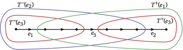
Figure 6. Useless edges cannot separate useful edges.

Proof.

Let $e_{1}$ and $e_{2}$ be useful edges. Let $e_{3}$ be an edge contained in the unique geodesic path between $e_{1}$ and $e_{2}$ and orient the path so it flows from $e_{1}$ to $e_{2}$ (see Figure 6). We show that $e_{3}$ is useful.

Since $e_{1}$ and $e_{2}$ are useful edges, neither $T^{+}(e_{1})$ nor $T^{-}(e_{2})$ contain all labels. By way of contradiction, suppose that $e_{3}$ is a useless. Then the vertices of either $T^{+}(e_{3})$ or $T^{-}(e_{3})$ contain all the labels. However, because $e_{3}$ lies between $e_{1}$ and $e_{2}$, we have $T^{+}(e_{3})\subset T^{+}(e_{1})$ and $T^{-}(e_{3})\subset T^{-}(e_{2})$. This means that either

$$\bigcup_{v\in T^{+}(e_{3})}\textnormal{Lab}(v)=S\subset\bigcup_{v\in T^{+}(e_{1})}\subsetneq S$$

or

$$\bigcup_{v\in T^{-}(e_{3})}\textnormal{Lab}(v)=S\subset\bigcup_{v\in T^{-}(e_{2})}\subsetneq S,$$

giving a contradiction. ∎

Recall that our ultimate aim is to associate edges in a Gromov approximating tree to splittings. For the proof of the main result, we are interested in nontrivial splittings. As we show in Section 6.4, an edge produces a nontrivial splitting when it is useful in the sense of Definition 5.7. For this reason, we let $T_{\textnormal{spl}}$ denote the subtree formed by useful edges.

Proposition 5.10.

Let $\textnormal{Lab}_{\textnormal{spl}}$ be the restriction of Lab to $T_{\textnormal{spl}}$. For nonempty $T_{\textnormal{spl}}$, the relation $\textnormal{Lab}_{\textnormal{spl}}$ is surjective (Definition 5.2, Property B).

Proof.

We assume that $T_{\textnormal{spl}}$ is nonempty. To show surjectivity of $\textnormal{Lab}_{\textnormal{spl}}$, we construct a tree $T^{\prime}$ by collapsing the useful subtree to a point: $T^{\prime}=T/T_{\textnormal{spl}}.$ Let $\rho_{\textnormal{spl}}:T\to T^{\prime}$ be the quotient map that induces the identification.

The image $v_{\textnormal{spl}}=\rho_{\textnormal{spl}}(T_{\textnormal{spl}})$ is a vertex of $T^{\prime}$. If $w$ is a vertex of $T^{\prime}$ other than $v_{\textnormal{spl}}$, it lifts to a unique vertex in $T\setminus T_{\textnormal{spl}}$. Hence we define $\textnormal{Lab}^{\prime}:\textnormal{vert}(T^{\prime})\to\{1,\dots,N\}$ to send $v_{\textnormal{spl}}$ to $\bigcup_{v\in T_{\textnormal{spl}}}\textnormal{Lab}(v)$ and other vertices $w$ to $\textnormal{Lab}(\rho_{\textnormal{spl}}^{-1}(w))$.

Since Lab is a labelling system, so is $\textnormal{Lab}^{\prime}$. Furthermore, every edge of $T^{\prime}$ is useless by construction. By Proposition 5.8, the tree $T^{\prime}$ has a full vertex $x$.

We claim that $x=v_{\textnormal{spl}}$. By contradiction, suppose that is it not. Then

$$\textnormal{Lab}(\rho_{\textnormal{spl}}^{-1}(x))=\{1,\dots,N\},$$

so the vertex $\rho_{\textnormal{spl}}^{-1}(x)$ of $T$ is full. By Proposition 5.8, the existence of a full vertex implies that all edges of $T$ are useless. This is a contradiction, as $T_{\textnormal{spl}}$ is nonempty. Hence $x=v_{\textnormal{spl}}$, and $\bigcup_{v\in T_{\textnormal{spl}}}\textnormal{Lab}(v)=\{1,\dots,N\}$. We conclude $\textnormal{Lab}_{\textnormal{spl}}$ is a surjective relation. ∎

6. Bounds on the displacement function

6.1. The space of discrete and faithful representations and the displacement function

An isometric action $G\curvearrowright\mathbb{H}^{n}$ is equivalent to a representation $\rho:G\to\textnormal{Isom}(\mathbb{H}^{n})$; the representation variety of $G$-actions on $\mathbb{H}^{n}$ is defined as

$$R(G,n)=\textnormal{Hom}(G,\textnormal{Isom}(\mathbb{H}^{n}))=\{\rho:G\to\textnormal{Isom}(\mathbb{H}^{n})\}.$$

We define the adjoint action $ad\curvearrowright\textnormal{Isom}(\mathbb{H}^{n})$ of $\textnormal{Isom}(\mathbb{H}^{n})$ on itself via conjugation: $ad(h)\cdot h^{\prime}=h^{-1}h^{\prime}h$. The adjoint action induces an action $\textnormal{Isom}(\mathbb{H}^{n})$ on $R(G,n)$; for $\rho\in R(G,n)$ and $h\in\textnormal{Isom}(\mathbb{H}^{n})$, the representation $h\cdot\rho$ sends $g$ to $h^{-1}\rho(g)h$. The space of conjugacy classes of representations in $R(G,n)$ is homeomorphic to the quotient

$$\overline{R}(G,n)=R(G,n)/\textnormal{Isom}(\mathbb{H}^{n}),$$

where $\textnormal{Isom}(\mathbb{H}^{n})$ acts on $R(G,n)$ by the action induced by $ad$.

Unfortunately, the above space is in general non-Hausdorff [Kap00, Section 4.3, p. 57]. So one instead considers the Mumford quotient

$$X(G,n)=\textnormal{Hom}(G,\textnormal{Isom}(\mathbb{H}^{n}))/\!/\textnormal{Isom}(\mathbb{H}^{n}),$$

which is an algebraic variety. The space $X(G,n)$ is called the character variety. For more information on this space, see [Mor86]. The series of work by Culler, Morgan, and Shalen [CS83][MS84][MS88a][MS88b][Mor86] examine the character variety.

We are interested in conjugacy classes of discrete and faithful actions on $\mathbb{H}^{n}$. Let

$$\textnormal{Hom}_{\textnormal{df}}(G,n)\subset\textnormal{Hom}(G,\textnormal{Isom}(\mathbb{H}^{n}))$$

denote the space of discrete and faithful representations. When $G$ does not contain any infinite nilpotent normal subgroups (e.g., it is not small), then

$$\textnormal{Hom}_{\textnormal{df}}(G,n)/\textnormal{Isom}(\mathbb{H}^{n})$$

is Hausdorff, and in particular, it is a subspace of both $\overline{R}(G,n)$ and the character variety $X(G,n)$ (see [Kap00, Chapter 8, p. 157]).

Definition 6.1.

Given a group $G$ and a dimension $n$, we define

$$\mathcal{D}(G,n)=\textnormal{Hom}_{\textnormal{df}}(G,n)/\textnormal{Isom}(\mathbb{H}^{n}),$$

and call this set the deformation space of $G$ into $\textnormal{Isom}(\mathbb{H}^{n})$.

Definition 6.2.

Let $G$ be a finitely-presented group generated by $S$. Let $\rho:G\to\textnormal{Isom}(\mathbb{H}^{n})$ be a representation, and let $B_{\rho}(x)=\max_{s\in S}d(x,s(x)).$ The displacement function of a representation is defined as $B_{\rho}=\inf_{x\in\mathbb{H}^{n}}B_{\rho}(x).$ We denote the supremum of displacement functions of representations in a deformation space as

$$B=\sup_{\rho\in\mathcal{D}(G,n)}B_{\rho}.$$

Given $[\rho],[\rho^{\prime}]\in\mathcal{D}(G,n)$, we have $B_{\rho}=B_{\rho^{\prime}}$ when $[\rho]=[\rho^{\prime}]$.

In [Bes88], Bestvina observed that the Compactness Theorem is equivalent to a uniform upper bound on the displacement function. As discussed in the introduction, the methods used to prove the Compactness Theorem do not give estimates for such a bound in general.

6.2. Application of combinatorial framework to special splittings

Let $W$ be a Coxeter group with system $(W,S)$, and $\rho:W\curvearrowright\mathbb{H}^{n}$ be a discrete, faithful, and isometric action. We associate this data to an approximating tree $T$. Below, we define the subset $X$ of $\mathbb{H}^{n}$ from which $T$ is constructed.

We assume that the Coxeter diagram $\Gamma(W,S)$ is connected; a disconnected Coxeter diagram corresponds to a splitting over the trivial group, which is small.

Let $S=\{s_{1},\dots,s_{k}\}$. Consider the set $\mathcal{S}$ of pairs $\{s_{i},s_{j}\}$ which generate finite dihedral groups. Being finite, these dihedral groups have nonempty fixed-point sets in $\mathbb{H}^{n}$ (see [BH99, Chapter II.6, Proposition 6.7]).

Fix a representation $\rho:W\to\textnormal{Isom}(\mathbb{H}^{n})$, and suppose it is discrete and faithful. Let $X$ be a set of representative points from the fixed-point sets of pairs in $\mathcal{S}$; hence $|X|\leq|\mathcal{S}|\leq\binom{k}{2}$.

Remark 6.3.

The space $X$ can have arbitrarily large diameter, even in the case $k=3$.

Let $(T,p)$ be a Gromov approximating tree for the set $X$, and recall the map $q:T_{\textnormal{sh}}\to T$. Let $\textnormal{stab}_{S}(x)$ denote the set of elements in $S$ that fix $x$.

Definition 6.4.

Let the labelling $\textnormal{Lab}:V(T)\to S$ send a vertex $v$ to the union of labels $\bigcup_{x\in p^{-1}(v)}\textnormal{stab}_{S}(x)$ when $q(v)\in X$ and to the empty set otherwise. We define a generator labelling denoted $\overline{\textnormal{Lab}}:V(T)\to S$ as the canonical extension of Lab.

Theorem 6.5.

The labelling $\overline{\textnormal{Lab}}:V(T)\to S$ is a labelling system.

Proof.

We show that the map $\overline{\textnormal{Lab}}$ is connected and surjective (Definition 5.2, Property A and Property B). The properties essentially hold by construction.

Property A follows from Lemma 5.5.

To show Property B, note that each $\rho(s_{i})$ has a nonempty fixed-point set because it is an involution. The diagram for $(W,S)$ is connected, so there exists an $s_{j\neq i}$ such that $\{s_{i},s_{j}\}$ generate a finite dihedral group, which has nonempty fixed point set. For each $s_{i}$, there is a point $x_{i}\in X$ fixed by $s_{i}$. Thus there is a point in $V(T)$ labelled by $s_{i}$, namely, the point $p(x_{i})$. Since $p(X)\subset V(T)$, it follows that the union $\bigcup_{v\in V(T)}\overline{\textnormal{Lab}}(v)$ contains the full set $S=\{s_{1},\dots,s_{g}\}$, so $\overline{\textnormal{Lab}}$ is surjective. ∎

6.3. Correspondence between the combinatorics of labelling systems and the geometry of actions

Let $\textnormal{Lab}:V(T)\to S$ and $\overline{\textnormal{Lab}}:V(T)\to S$ be the maps defined in Definition 6.4.

The combinatorics of the generator labelling system $\overline{\textnormal{Lab}}$ correspond to the geometry of the action: if $s_{i}$ labels a vertex $v\in T$, then we can bound the amount by which $\rho(s_{i})$ displaces its shadow $q(v)$. To make this statement precise, we introduce the notion of an $R$-fixed point.

Definition 6.6.

Let $R\geq 0$. Fix an action $W\curvearrowright\mathbb{H}^{n}$. We say a point $x$ is $R$-fixed by elements $w_{1},\ldots,w_{m}$ of $W$ if

$$d(x,w_{i}(x))\leq R\textrm{ for all }i\in\{1,\ldots,m\}.$$

Proposition 6.7.

Let $s\in S$. Suppose $u,w$ are vertices in $T$ and $x,y$ are vertices in $T_{\textnormal{sh}}$ so that $P(x)=u$, $P(y)=w$, and $s\in\textnormal{Lab}(u)\cap\textnormal{Lab}(w)$. If $z\in[xy]_{\textnormal{sh}}$, then $z$ is $R$-fixed by $s$, where $R=2^{8}(|X|(20c\delta+12\delta)+4c\delta)$.

As a consequence of Proposition 6.7, we obtain:

Proposition 6.8.

Suppose that $v$ is a vertex of $T$ and $s\in\overline{\textnormal{Lab}}(v)$. Then $q(v)$ is $R$-fixed by $s$, where $R$ is defined as in Proposition 6.7.

Proof.

If $s\in\overline{\textnormal{Lab}}(v)$, then by Lemma 5.4, there are vertices $u,w\in T$ and $x,y\in T_{\textnormal{sh}}$ such that $v\in[uw]$, $s\in\textnormal{Lab}(u)\cap\textnormal{Lab}(w)$, and $p(x)=u,p(y)=w$. Since $x$ and $y$ are fixed by $s$, it follows from Proposition 6.7 that the vertex $q(v)$ is $R$-fixed by $s$. ∎

Proof of Proposition 6.7..

We use the following lemma.

Lemma 6.9 ([Kap00, Lemma 3.43, pp. 48-49]).

Let $\gamma=[xy]_{\mathbb{H}}$ be a geodesic and $\widehat{\gamma}$ be an $(1,A)$-quasi-geodesic path from $x$ to $y$. Then $\widehat{\gamma}$ is contained in a regular $r$-neighbourhood $N_{r}(\gamma),$ where $r=2^{7}A.$

Let $\gamma=[xy]_{\mathbb{H}}$ and $\widehat{\gamma}=[xy]_{\textnormal{sh}}$. We claim that $\widehat{\gamma}$ is a $|X|(20c\delta+12\delta)+4c\delta$ quasi-geodesic. To show this, let $P_{\gamma}:Q(X)\to T$ be a map sending $\gamma$ to $[uw]$ satisfying the conditions of Lemma 3.11. The map $P_{\gamma}$ is distance decreasing on elements of $X$. Let $z_{1}$ and $z_{2}$ be the unique points of $\overline{X}$ such that $p(x)=p(z_{1})$ and $p(y)=p(z_{2})$. Let $\widehat{\gamma}^{\prime}$ be the segment of $\widehat{\gamma}$ contained in the image of $q$; it is a sequence of edges of $T_{\textnormal{sh}}$ connecting $z_{1}$ to $z_{2}$. Recall that when restricted to each edge, the map $q$ is a $(1,20c\delta+12\delta)$-quasi-isometry which is a homeomorphism. Thus, we can construct a $(1,|X|(20c\delta+12\delta))$-quasi-isometry $\alpha:\widehat{\gamma}^{\prime}\to[uw]$ by defining $\alpha$ as $q^{-1}$ along edges. Then $q\circ P_{\gamma}$ sends $\gamma$ to $\widehat{\gamma}^{\prime}$, so the length of $\widehat{\gamma}^{\prime}$ is at most $d_{\mathbb{H}}(x,y)+|X|(20c\delta+12\delta)$.

By construction of $T_{\textnormal{sh}}$ (Definition 4.4) and the definition of a Gromov approximating tree (Definition 3.6, Property 2), points in $T_{\textnormal{sh}}$ not contained in $q(T)$ are at most $2c\delta$ away from $q(T)$. Since the shortest path between $x$ and $y$ is at least as long as $d_{\mathbb{H}}(x,y)$, it follows that

$$d_{\mathbb{H}}(x,y)\leq d_{\textnormal{sh}}(x,y)\leq d_{\mathbb{H}}(x,y)+|X|(20c\delta+12\delta)+4c\delta.$$

Set $A=|X|(20c\delta+12\delta)+4c\delta$. Let $a$ be a point on $\widehat{\gamma}$. Let $b$ be the nearest point on $\gamma$ to $a$. The element $s$ fixes $x$ and $y$, so $s$ fixes $\gamma$ and sends $[ab]_{\mathbb{H}}$ to $[s(a)b]_{\mathbb{H}}$. The distance $d(a,b)=d(s(a),b)$ is bounded above by $r=2^{7}A$ as a consequence of Lemma 6.9. It follows that $d(a,s(a))$ is bounded above by $R=2^{8}A$.

We have shown that all points of $\widehat{\gamma}$ are $R$-fixed by $s$. ∎

6.4. Special splittings produced by Gromov approximating trees

An edge $e$ of the Gromov approximating tree $T$ determines a special splitting in the following way.

Proposition 6.10.

Define sets of generators

$$S^{+}(e)=\bigcup_{v\in T^{+}(e)}\{s\in\textnormal{Lab}(v)\},$$

$$S^{-}(e)=\bigcup_{v\in T^{-}(e)}\{s\in\textnormal{Lab}(v)\},$$

$$S^{*}(e)=S^{+}(e)\cap S^{-}(e).$$

The special splitting $\langle{S^{+}(e)}\rangle\ast_{\langle{S^{*}(e)}\rangle}\langle{S^{-}(e)}\rangle,$ where the amalgamation maps are induced by the inclusions $S^{*}(e)\hookrightarrow S^{\pm}(e)$, yields a group isomorphic to $W$. Furthermore, the splitting is trivial if and only if $e$ is useless, i.e., either $S^{+}(e)=S$ or $S^{-}(e)=S$.

Proof.

Let $\Gamma$ denote the Coxeter diagram for the system $(W,S)$. We let $\Gamma^{*}\subset\Gamma$ denote the subgraph spanned by $S^{*}(e)$; we define $\Gamma^{+}$ and $\Gamma^{-}$ similarly.

By Proposition 1.11, it suffices to show that $\Gamma^{*}$ separates $\Gamma$ and that $S\subset S^{+}(e)\cup S^{-}(e)$.

We first show that $\Gamma^{*}$ separates $\Gamma$. Let $\gamma$ be a path from $\Gamma^{+}\setminus\Gamma^{*}$ to $\Gamma^{-}\setminus\Gamma^{*}$. By way of contradiction, suppose that $\gamma$ does not pass through $\Gamma^{*}$. Then $\gamma$ contains vertices $s_{+}\in S^{+}(e)\setminus S^{*}(e)$ and $s_{-}\in S^{-}(e)\setminus S^{*}(e)$ that are connected by exactly one edge in $\Gamma$. Hence the group $\langle{s_{+},s_{-}}\rangle$ is a finite dihedral group, and $\{s_{+},s_{-}\}$ is an element of $\mathcal{S}$. So $\{s_{+},s_{-}\}$ is contained in either $S^{+}(e)$ or $S^{-}(e)$. Without loss of generality, suppose that $\{s_{+},s_{-}\}\subset S^{+}(e).$ Then $s_{-}\in S^{+}(e)\cap S^{-}(e)=S^{*}(e)$. This contradicts the assumption that $s_{-}\in S^{-}(e)\setminus S^{*}(e)$.

We have shown that $\langle{S^{+}(e)}\rangle\ast_{S^{*}(e)}\langle{S^{-}(e)}\rangle$ is a splitting. To complete the proof, it remains to show that $W\cong\langle{S^{+}(e)}\rangle\ast_{S^{*}(e)}\langle{S^{-}(e)}\rangle$. It suffices to check that $S^{+}(e)\cup S^{-}(e)=S$. This follows from the surjectivity of $\overline{\textnormal{Lab}}$. Hence an edge $e$ determines the desired splitting. ∎

The splitting over $e$ may be trivial. In Section 6.5, we find a lower bound on the displacement function of a representation to ensure the existence of a nontrivial splitting.

6.5. Lower bound on the displacement function to guarantee existence of nontrivial splittings

Proposition 6.11.

If every edge of $T$ determines a trivial splitting of $W$, then $T_{\textnormal{sh}}$ contains a point that is $R$-fixed by all generators in $S$. Hence if $B_{\rho}>R$, there exists a nontrivial splitting of $W$.

Proof.

Suppose that every edge of $T$ determines a trivial splitting. Then every edge of $T$ is useless. By Proposition 5.8, there exists a vertex $v\in T$ labelled by the full set $S=\{s_{1},\dots,s_{k}\}$. By Proposition 6.8, the point $q(v)\in V(T_{\textnormal{sh}})$ is $R$-fixed by $S$.

If a point in $\mathbb{H}^{n}$ is $R$-fixed by $S$, then $B_{\rho}\leq R$. This follows from the definition of the displacement function and the definition of an $R$-fixed point. This means that when $B_{\rho}>R$, there exists an edge $e$ which is useful and thus determines a nontrivial splitting of $W$. ∎

By Proposition 5.9, the union of edges of $T$ which determine non-trivial splittings of $W$ is connected.

Definition 6.12.

Let $T_{\textnormal{spl}}$ denote the subtree consisting of the union of useful edges and call this subtree the useful subtree.

Theorem 6.13 (Useful subtree theorem).

When $B_{\rho}>R$, the useful subtree $T_{\textnormal{spl}}$ is nonempty.

Proof.

By Proposition 6.11, there exists a useful edge $e$ of $T$. Hence $T_{\textnormal{spl}}$ is nonempty. ∎

7. Small decompositions

In this section, we prove the main result of the paper.

Let $\mu_{n}$ be the Kazhdan-Margulis constant for $\mathbb{H}^{n}$ (Theorem 2.2).

Effective Compactness Theorem for Coxeter groups.

Let $(W,S)$ be a Coxeter system and suppose $S$ has $k$ elements. There exists a function $C_{n}(k)$ with the property that either $W$ has a small special nontrivial splitting or the displacement function is bounded above by $C_{n}(k)$ for every discrete and faithful $W$-action on $\mathbb{H}^{n}$. We may take

$$C_{n}(k)=R+2\binom{k}{2}\Lambda(\mu_{n},R),$$

where $R=2^{8}(\binom{k}{2}(20c\delta+12\delta)+4c\delta)$, and $\Lambda(\mu_{n},R)=2\binom{k}{2}(\frac{4}{\mu_{n}}+2R)$ (as defined in Proposition 2.3).

As a function of $k$, the estimate $C_{n}(k)$ is of order $k^{4}$.

Definition 7.1.

We say that the shadow length of an edge $e$ in $T$ is the length of the quasi-geodesic segment $q(e)\subset T_{\textnormal{sh}}\subset\mathbb{H}^{n}$. We let $|q(e)|$ denote the shadow length of $e$. (See Proposition 4.1 for the definition of the map $q$.)

We seek a condition on the shadow length of a useful edge $e$ that guarantees the existence of a small nontrivial splitting of $W$ (Definition 2.1).

Let $\Lambda_{n}=\Lambda(\mu_{n},R)$, where $R$ is defined as in Proposition 6.8. Given an action $\rho:W\curvearrowright\mathbb{H}^{n}$ and an edge $e$ of $T$, we define $S^{*}(e)$ as in Section 6.4.

Lemma 7.2.

If $|q(e)|\geq\Lambda_{n},$ then then $S^{*}(e)$ generates a small group and the special splitting associated with $e$ is small.

Proof.

Let $m$ be the midpoint of $q(e)$. We show that $m$ is $\mu_{n}$-fixed by $S^{*}(e)$. According to Proposition 6.8, if $s\in S^{*}(e)$, then the shadow of each vertex in $e$ is $R$-fixed by $s$. Therefore, since $|q(e)|\geq\Lambda_{n}$, it follows from Proposition 2.3 that $d(m,s(m))\leq\mu_{n}$ for all $s\in S^{*}(e)$. The representation $\rho(\langle{S^{*}(e)}\rangle)\subset\textnormal{Isom}(\mathbb{H}^{n})$ is discrete, so by the Kazhdan-Margulis Lemma (Theorem 2.2), the group $\rho(\langle{S^{*}(e)}\rangle)$ is small. Since $\rho$ is a faithful representation, we conclude that $S^{*}(e)$ generates a small group. ∎

Lemma 7.3.

There exists a function $C_{n}(k)$ with the following property. If the shadow length of every edge in $T_{\textnormal{spl}}$ is less than or equal to $\Lambda_{n}$, then each $x\in q(T_{\textnormal{spl}})$ is $C_{n}(k)$-fixed by $S$. Furthermore, we may take

$$C_{n}(k)=R+2\binom{k}{2}\Lambda_{n}=2^{8}\left(\binom{k}{2}(20c\delta+12\delta)+4c\delta\right)+2\binom{k}{2}\Lambda_{n}.$$

Proof.

If $T_{\textnormal{spl}}$ is empty, then the lemma holds trivially, so we work with nonempty $T_{\textnormal{spl}}$.

Let $x$ be a point in $q(T_{\textnormal{spl}})$, and let $s_{i}$ be an element of $S$. We analyse how far $s_{i}$ displaces $x$.

By Proposition 5.10, there is a vertex $v_{i}$ of $T_{\textnormal{spl}}$ with $s_{i}\in\overline{\textnormal{Lab}}(v_{i})$. Since $|q(e)|\leq\Lambda_{n}$ for each edge $e$ of $T_{\textnormal{spl}}$, the distance $d(x,q(v_{i}))$ is bounded above by $E\Lambda_{n}$, where $E$ is maximum number of edges in a geodesic path in $T_{\textnormal{spl}}$.

Set $R=26c\delta+12\delta$. The distance between $q(v_{i})$ and $s_{i}(q(v_{i}))$ is bounded above by $R$, by Proposition 6.8. It follows that

$$d(x,s_{i}(x))\leq 2d(x,q(v_{i}))+R\leq R+2E\Lambda_{n}.$$

Since the value of $E$ is bounded above by $\binom{k}{2}$, we conclude that $x$ is $C_{n}(k)$-fixed by $S$, where $C_{n}(k)=R+2\binom{k}{2}\Lambda_{n}.$ ∎

It follows that if all edges of $T_{\textnormal{spl}}$ have length less than or equal to $\Lambda_{n}$, then $B_{\rho}\leq C_{n}(k)$.

Proof of the Effective Compactness Theorem for Coxeter Groups.

Let $C_{n}(k)$ be the function defined in Lemma 7.3, and suppose that $B_{\rho}>C_{n}(k).$ Then $\mathbb{H}^{n}$ contains no point $C_{n}(k)$-fixed by $S$. The useful subtree theorem (Theorem 6.13) guarantees that $T_{\textnormal{spl}}$ is nonempty, as $B_{\rho}>C_{n}(k)>R$. Since $T_{\textnormal{spl}}$ is nonempty, Lemma 7.3 guarantees the existence of an edge $e$ of $T_{\textnormal{spl}}$ whose shadow length is greater than $\Lambda_{n}$. By Proposition 6.10, the special splitting determined by $S^{*}(e)$ is nontrivial. By Lemma 7.2, this splitting is small.

Thus either $W$ admits a small special nontrivial splitting or $B_{\rho}\leq C_{n}(k)$ for every $[\rho]\in\mathcal{D}(W,n)$. ∎

References

[Bar07] J. Barnard. Bounding surface actions on hyperbolic
spaces, arXiv:0709.2722.
[Bes88] M. Bestvina. Degenerations of the hyperbolic space.
Duke Math. J., 56(1): 143–161, 1988.
[BF95] M. Bestvina and M. Feighn. Stable actions of groups
on real trees. Invent. Math., 121: 287–321 (1995).
[BH99] M. Bridson and A. Haefliger. Metric Spaces
of Non-Positive Curvature. Springer-Verlag, Berlin, 1999.
[CDP90] M. Coornaert, T. Delzant, and A. Papadopoulos. Géométrie
et théorie des groups: les groups hyperboliques de Gromov.
Lecture notes in mathematics 1441, Springer, 1990.
[CS83] M. Culler and P. Shalen. Varieties of group representations
and splittings of 3-manifolds. Ann. of Math., (2) 117(1): 109–146, 1983.
[Deb70] H. E. Debrunner.
Helly Type Theorems Derived From Basic Singular Homology.
Amer. Math. Monthly, 77(4): 375–380, 1970.
[Del95] T. Delzant. L’image d’un groupe dans un groupe
hyperbolique. Comment. Math. Helvetici, 70: 267-284, 1995.
[GD90] E. Ghys and P. De la Harpe. Sur les espaces
hyperbolique d’après
Mikhael Gromov. Progr. Math. 83, Birkhäuser, Boston, 1990.
[Kap00] M. Kapovich. Hyperbolic Manifolds and Discrete
Groups. Birkhäuser, 2000.
[KM68] D. Kazhdan and G. Margulis. A proof of Selberg’s
hypothesis. Math. Sbornik, 75: 162–168, 1968.
[MT07] M. Mihalik and S. Tschantz.
Visual Decompositions of Coxeter Groups. arXiv:math.GR/0703439.
[Mor86] J. Morgan.
Group actions on trees and the compactification
of the spaces of classes of -representations.
Topology, 25: 1–34, 1986.
[MS84] J.W. Morgan and P.B. Shalen. Valuations, trees, and
degenerations of hyperbolic structures I. Ann. of Math.(2), 120(3): 401-476, 1984.
[MS88a] J.W. Morgan and P. B. Shalen. Degenerations of hyperbolic structures, II: Measured laminations in 3-manifolds.
Ann. of Math.(2), 127(2): 403–456, 1988.
[MS88b] J.W. Morgan and P. B. Shalen. Degenerations of hyperbolic structures, III: Actions of 3-manifold groups on trees and Thurston’s compactness theorem. Ann. of Math.(2), 127(3): 457–519, 1988.
[Ser03] J. P. Serre. Trees. Springer-Verlag, New York (2003).
[Thu86] W.P. Thurston. Hyperbolic Structures
on 3-Manifolds I: Deformation of Acylindrical Manifolds. Ann. of
Math.(2), 124(2): 203–246, 1986.