The Internal Kinematics of the HII Galaxy II Zw 40 (catalog )

Abstract

We present a study of the kinematic properties of the ionized gas in the dominant giant Hii region of the well known Hii galaxy: II Zw 40. High spatial and spectral resolution spectroscopy has been obtained using IFU mode on the GMOS instrument at Gemini-North telescope. The observations allow us to obtain the H$\alpha$ intensity map, the radial velocity and velocity dispersion maps as well as estimate some physical conditions in the inner region of the starburst, such as oxygen abundance (O/H) and electron density. We have used a set of kinematics diagnostic diagrams, such as the intensity $versus$ velocity dispersion (I-$\sigma$), intensity $versus$ radial velocity (I-V) and $V$-$\sigma$, for global and individual analysis in sub-regions of the nebula. We aim to separate the main line broadening mechanisms responsible for producing a smooth supersonic integrated line profile for the giant Hii region. Bubbles and shells driven by stellar winds and possibly supernovae, covering a large fraction on the face of the nebula, are identified on scales larger than 50 pc. We found that unperturbed or “free from shells” regions showing the lowest $\sigma$ values ($\sim$ 20 km s^-1) should be good indicators for the $\sigma_{grav}$ component in II Zw 40. The brightest central region (R $\sim$ 50 pc) is responsible for $\sigma$ derived from a single fit to the integrated line profile. The dominant action of gravity, and possibly unresolved winds of young ($<$10 Myr) massive stars, in this small region should be responsible for the characteristic H$\alpha$ velocity profile of the starburst region as a whole ($\sigma$ = 32-35  $\hbox{km}\thinspace\hbox{s}^{-1}$). Our observations show that the complex structure of the interstellar medium of this galactic scale star-forming region is very similar to that of nearby extragalactic giant Hii regions in the Local Group galaxies.

1 Introduction

Hii galaxies (HiiGs) are dwarf galaxies undergoing a burst of star formation. Their extensive star-forming regions, composed of an ensemble of Super Star Clusters (SSC) and giant Hii regions (GHiiRs), dominate the optical emission. HiiGs represent the simplest examples of the starburst phenomenon occurring on galactic scales. II Zw 40 is one of the most famous HiiG showing an intense starburst in its central region. Its optical spectrum is dominated by very intense emission lines of H, He, [O ii], [O iii], [N ii], [S ii] and [Ne iii] superposed on a faint blue continuum, indicating that the present rate of star formation (SF) is much higher than the historical average (Sargent & Searle, 1970; Searle & Sargent, 1972; Terlevich et al., 1991; Walsh & Roy, 1993; Kehrig et al., 2004). II Zw 40 has a subsolar oxygen abundance of 12+log(O/H)=8.07 from the data of Kehrig et al. (2004), typical of this class. The star formation (SF) history of this galaxy has been the object of several studies, ranging from the hypothesis that the star-forming episode may be producing a first generation of stars, to a scenario in which the history of SF consists of a continuous series of short bursts over its lifetime. Near infrared spectra have been obtained by Vanzi et al. (1996), who showed that II Zw 40 has low supernova rate and that no nuclear starburst, as powerful as the present one, has occurred in the past Giga-year. Kunth & Sargent (1981) and Vacca & Conti (1992) found Wolf-Rayet (WR) features in the optical spectrum, confirming that the central region is very young (3-6 Myr). Beck et al. (2002) found that the bright central region concentrate 75% of the thermal free-free emission and that the 75 pc region is formed by four supernebula each powered by $\sim$ 600 O stars. Ulvestad et al. (2007) also found no radio supernovae with powers greater than Cas A.

The initial trigger of the present SF episode is also a question that remains unanswered for this class of dwarf starbursts since most are isolated systems (Telles & Terlevich, 1995; Telles & Maddox, 2000). If not triggered by external agents (i.e. interactions), star formation is caused by internal processes manifesting in a stochastic manner (Pelupessy et al., 2004). This may be the case for the subsample of low luminosity, compact objects, classified as type II HII galaxies by Telles, Melnick & Terlevich (1997), with no signs of morphological disturbances. However, the more luminous HII galaxies, classified as type I, do show some signs of extensions, fuzz, or tails in their outer envelopes, suggesting tidal origin. Over the years, only a few studies have been carried out to determine the overall dynamics of II Zw 40. Hi velocity mapping reveals complex structure with a subtle velocity gradient (Brinks & Klein, 1988; van Zee et al., 1998). The southeast and northwest Hi tails have reversal rotation, suggesting that most of the material is falling back toward the dynamical center. The best scenario for the formation of II Zw 40 seems to be the result a collision between two gas-rich dwarf galaxies, and the current starburst occurs in the overlapping merging region (Baldwin et al., 1982).

In the early 70’s, Smith & Weedman (1970a, 1972) first discovered broad [OIII] and Balmer lines in GHiiRs. These lines have widths which are broader (i.e. line of sight velocity dispersion $\sigma\sim 13-25$  $\hbox{km}\thinspace\hbox{s}^{-1}$) than those found in normal Hii regions in the Galaxy, e.g. $\sigma$ $\sim$ 5.4 km s^-1 in Orion (Münch, 1958; Smith & Weedman, 1970b). These high velocity widths imply gas motions a few times the speed of sound. The early detailed studies suggested that winds from WR stars should contribute to the total kinetic energy in mass motions (Smith & Weedman, 1972), and that supernova remnants (SNRs) could play a significant role in the energetic balance of GHiiRs (Skillman & Balick, 1984).

In the meantime, Melnick (1977) showed a correlation between the diameter and the global H$\alpha$ profile widths of GHiiRs. Terlevich & Melnick (1981) found L(H$\beta)\propto\sigma^{\sim 4}$ which led them to propose a gravitational model for the origin of the supersonic motions, due to the close similarities with the parametric relations found for systems in dynamical equilibrium, such as elliptical galaxies, globular clusters and bulges of spiral galaxies. The first extrapolation to HiiGs was done by Melnick et al. (1988), where a significant sample of galaxies was observed, including II Zw 40. Recent work also confirms the existence of the $L$-$\sigma$ relation for HiiGs, suggesting that GHiiRs and the star-forming regions in HiiGs belong to a single family of objects (Rozas et al., 2006; Bosch et al., 2002; Telles et al., 2001; Fuentes-Masip et al., 2000).

Several line broadening mechanisms have been proposed to interpret the supersonic widths measured in the spectra of GHiiRs and HiiGs. Dyson (1979) proposes that line profiles consist of two components: one broad line component of the shocked region, and a narrower component originated in the neighboring region which is ionized by UV photons escaping from the broad line region. The broad line emission is likely to arise near the shell of a hot ($10^{6}$K) highly ionized, wind-driven bubble. Yorke et al. (1984) used the champagne flow model (Tenorio-Tagle, 1979) – disruption of neutral clouds adjacent to Hii regions– to explain the broad lines. The gravitational model (Terlevich & Melnick, 1981) is based on the assumption that the dominant influence is the gravitational potential. In this model, the observed Gaussian line profiles are a direct consequence of the virialized motions of the gas plus stars complex. If one supposes a self gravitating system, the standard deviation of this Gaussian profile in velocity is

$$\sigma\sim\sqrt{\frac{GM}{R}}.$$

The Cometary Stirring Model (CSM) proposed later by Tenorio-Tagle et al. (1993) improves the simpler original picture. They propose that a group of pre-main-sequence low-mass stars of a recently formed starburst, move under the gravitational potential with velocity dispersion $\sigma_{star}$. These stars drive winds that stir the remaining cloud through supersonic bow, or “cometary”, shocks, providing it with an average turbulent motion $\sigma_{gas}$ $\sim$ $\sigma_{star}$. This model estimates the total power of the shocks and associated line the luminosity which agree with the observed relation L $\sim$ $\sigma^{4}$. Few attempts have been made (e.g. Östlin et al., 2004; Cumming et al., 2008), and none with a statistically significant sample, to definitely test the hypothesis of $\sigma_{gas}=\sigma_{star}$ which would strengthen the support for this model.

A skeptical view of this scenario was presented by Chu & Kennicutt (1994) in a detailed study of the GHiiR 30 Doradus in the Large Magellanic Cloud (LMC). They showed that a smooth integrated velocity profile in the inner region (135 $\times$ 135 pc) results from a complex velocity field, which demonstrates the futility of using global velocity profiles to infer the physical origin of the gas motion. The dominant contributor to the global velocity dispersion, as proposed by the authors, at least in the bright core, is the superposition of individual expanding shells. Consequently, the most important physical mechanisms would be the stellar winds from OB associations combined with champagne-type flows and possibly supernovae.

This long disagreement in the literature has also been enlightened by works favored by high spectral, spatial as well as bi-dimensional spectroscopy of GHiiRs and the nearest HiiGs. Muñoz-Tuñón et al. (1996) analyzed the velocity field of NGC 604 and NGC 588 in the galaxy M33. They show that, in both cases, the peaks of high velocity dispersions are systematically concentrated in regions of faint nebular emission. On the other hand, there is a smooth low velocity dispersion component which permeates all regions of the nebula. They proposed a simple criterion to identify expanding shells in the intensity vs. $\sigma$ diagram. This smooth low velocity dispersion component is what one measures in the integrated spectrum of a GHiiR. Yang et al. (1996) came up with basically the same conclusions in a similar study of NGC 604. The results found by Telles et al. (2001) using Echelle long-slit spectroscopy of a small sample of HiiGs point in the same direction. Despite the complex velocity fields found in such objects, they show that the brightest knots dominate the global luminosity and velocity dispersion.

Though much effort has been spent to understand the kinematics of the gas-stars complex in GHiiRs and HiiGs, a clear picture is still absent, given the complexity of these systems. The puzzle can be noted in the follow question: Why should one find such parametric relations in these violent environments where massive star evolution seems to play a significant, maybe dominant, role? Here, we aim to bring some insight to this question by extending the bi-dimensional spectroscopy study of Local GHiiRs to this nearby prototypical HiiG, with comparable spatial and spectral resolution. The kinematics of the ionized gas in the very center of II Zw 40 is investigated in some detail.

II Zw 40 has coordinates R.A. 05^h 55^m 42^s.6, DEC. +03^o 23^m 32$\arcsec$ (J2000.0), a V = 15 mag (Telles & Terlevich, 1997). It lies at a low galactic latitude of $\sim-10$ degrees. The observed radial velocity of 778  $\hbox{km}\thinspace\hbox{s}^{-1}$  and a cosmological (corrected from heliocentric to cosmic microwave background frame) recession velocity of 845  $\hbox{km}\thinspace\hbox{s}^{-1}$, puts it at a distance of 11.9 Mpc.

The paper is organized as follows. Section 2 describes the observations and reduction procedures. The results are presented in § 3 together with full descriptive data analysis. In § 4 we discuss our results. Finally, we give a brief summary in § 5.

2 Observations and Data Reduction

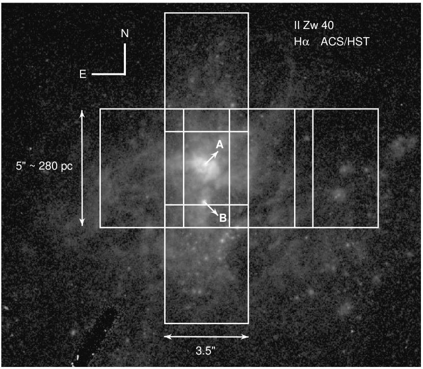
Figure 1: A high resolution H$\alpha$ image (0.027″/pixel) obtained with ACS/HST. The GMOS/IFU fields are shown over the central region of the galaxy (HST’s archive data from the proposal 9739 by Rupali Chandar; see also Figure 1 in Vanzi et al. (2008)).

The observations of II Zw 40 were done during the run GN-2003B-Q-26 on 2003 December 26. We used GMOS equipped with an Integral Field Unit (IFU) on the Gemini-North Telescope. The IFU was used in one-slit mode giving a 3.5 $\times$ 5 arcsec² field of view. Each lens in its original hexagonal shape has 0.2$\arcsec$ nominal size projected in the sky. In this case, the IFU directed to the science target has 20 $\times$ 25 lenses, in a total of 500 lenses. A set of 249 lenses, 1 arcmin away from the science target, provides a sky background for subtraction during the data reduction. In order to cover a larger field, we exposed at six different offsets overlapping the fields about 1$\arcsec$. Figure 1 shows the ACS/HST high resolution H$\alpha$ image (0.027 arcsec/pixel), with the different fields observed with GMOS/IFU shown as rectangles over the image. The GMOS/IFU data were recorded in three 2048 $\times$ 4608 CCDs with 13.5$\mu$m pixel size. We used the R831 grating covering the wavelength range 5970-8080Å and providing a spectral resolution of 1.5Å (FWHM) at 6580Å, with corresponding $\sigma_{inst}$ = 29.0$\pm$1.0 km s^-1 ($\sigma$=FWHM/2.355). The exposure time of each field was 300 seconds. The seeing remained constantly sub-arcsecond during the observations ($\approx$ 0.5-0.6$\arcsec$).

The basic data reduction was performed using the Gemini IRAF package developed by the Gemini Observatory staff. A CuAr spectrum was obtained in order to provide the wavelength calibration. We processed bias subtraction, dome and twilight flat field correction. Each field was calibrated in wavelength but not in flux. The final cube for each field was re-sampled to 0.2 arcsec per pixel using GFCUBE, resulting in a 16 $\times$ 25 $\times$ 6270 data cube. We developed a special procedure using IRAF in order to produce the H$\alpha$ emission, radial velocity and velocity dispersion synthetic maps. For each data cube we used the task FITPROFS in onedspec package to fit a single Gaussian profile to the H$\alpha$ emission line. The task provides the H$\alpha$ central wavelength, the FWHM and the integrated intensity in relative counts. We run the task automatically for all spectra in the original sampling (0.2$\arcsec$ hexagonal spaxel) and re-sampled (0.2$\arcsec$/pixel) data cubes. There is no difference using either data sets, nevertheless, it is more practical for the analysis to use the re-sampled square pixel data cubes. We constructed FITS images using H$\alpha$ line intensities, centers and FWHM values to build our final maps. Finally, we overlapped them to build the mosaiced field.

As an additional test, the different maps were also produced from the original data cube using the ADHOC package (Boulesteix, 1999) in a parallel reduction procedure in order to check the accuracy of the data reduction. This package is designed to reduce Fabry-Perot interferometry data and is able to handle any data cube. Both reductions showed very similar maps, then we decided to use the maps produced with the IRAF routines for all our further analysis.

Figure 2 shows a spectrum of a single pixel on the brightest region on the main knot of II Zw 40 nebula (knot A). This one pixel spectrum illustrates the quality of our data, and shows that we are able to detect, resolve and measure faint lines of [OI]$\lambda$6300, [SIII]$\lambda$6312, [NII]$\lambda\lambda$6548,6584, HeI$\lambda$6678, [SII]$\lambda\lambda$6717,6731, [NeI]$\lambda$7024, HeI$\lambda$7065, [ArIII]$\lambda$7136, HeI$\lambda$7281, [OII]$\lambda\lambda$7318, [OII]$\lambda\lambda$7330, and [ArIII]$\lambda$7751(not shown). The peak intensity of H$\alpha$ in this one single pixel exceeds 7000 counts and with a total flux of 20000 counts. The S/N on the continuum around H$\alpha$ (which is not of interest here) is about 5 on this one pixel spectrum. On the fainter regions, where the line widths are still measurable, the S/N on the adjacent continuum is about 0.5, and what determines the accuracy of the line width measurement is the peak intensity over the continuum which is directly proportional to the total flux of the emission line. We estimated, therefore, a conservative minimum relative flux necessary to accurately measure a single H$\alpha$ line width of 300 counts (log F = 2.5).

The single Gaussian fit is an operational measurement procedure. Though the major contribution comes from regions presenting line profiles well fitted by single Gaussians, some regions of the nebula show asymmetric line profiles or multiple components. These measurements can map regions of kinematic interest through line width variations, and can reveal large scale motions through variations of the line centroids across the nebula. When one has sufficient high spectral resolution the analysis of a single line profile can provide additional information constraining the larger and the smaller scale velocity variations.

3 Results

3.1 Electron density and abundance distribution

We briefly comment on the distribution of some derived physical properties before we proceed with the main topic of the kinematic properties of the starburst region in II Zw 40. We have been able to reliably measure and map the distribution of some weak lines in the central field.

Figure 3 shows the electron density (n_e) distribution derived from the ratio of [SII]$\lambda\lambda$6717,6731 lines (Dopita & Sutherland, 2003). This plot was produced by azimuthally averaging the 2D map centered on the peak distribution of the sulfur line ratio which is coincident with the peak H$\alpha$ line emission from knot A. Firstly, we show that n_e is not constant and ranges from $\sim$1400 cm^-3 in the center to $\sim$ 500 cm^-3 about 100 pc from the center of knot A, and higher than the low density limit of 100 cm^-3. It is also noticeable the good fit to a r^1/4 law (solid line) to the outer points (avoiding the dominant effect of seeing in the center represented by the dotted line), which is usually representative of the surface brightness distribution of stellar systems in dynamical equilibrium.

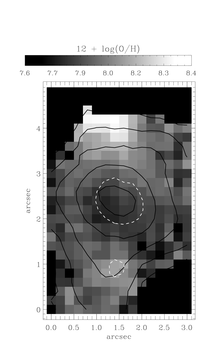
Figure 4: Oxygen abundance distribution in the central field, derived from the ratio of [NII]$\lambda$6584/H$\alpha$ (Denicoló et al., 2002). The H$\alpha$ emission contours at 68, 20, 9, 5 and 3.4% of the peak intensity (solid lines) and the continuum emission contours (dashed lines) at 47% of its peak intensity are superposed on the image. We use a 3$\times$3 box smooth the pixel-to-pixel variation due to poisson noise

Figure 4 shows the oxygen abundance distribution in this central field. H$\alpha$ and continuum emission are also plotted as contours over the image. All pixels with H$\alpha$ emission less than 3.4% of the peak emission were erased. The O/H abundance was derived by applying the N2 calibrator from Denicoló et al. (2002). This is an empirical relation between the the line ratio of [NII]$\lambda$6584/H$\alpha$ with the oxygen abundance. Simple closed box chemical evolution models considering the primary and secondary origin of nitrogen predict this linear correlation between nitrogen and oxygen, though dependent on the ionization parameter. Here, we simply apply the empirical calibration of this relation. We found a lower abundance over knot A, 12+log(O/H) = 7.85, a slight increase over knot B, 12+log(O/H) = 8.0 and a significant increase in a region at NE of the knot A, 12+log(O/H) = 8.3. The statistical error of the N2 estimator is $\delta_{(\rm{O/H})}\sim 0.15$, however relative differences between the regions should be real.

We will not explore the physical conditions analysis here any further. However, we may say that we have not found any relation between the velocity dispersion and the oxygen abundance or n_e.

3.2 The H$\alpha$ Integrated Line Profile

We now compare the integrated line width for the main starburst region in II Zw 40 derived here, with the inner core line width obtained with the high dispersion fiber spectrograph FEROS (Kaufer et al., 1999), on the 1.52m telescope (ESO). We combined 181 spectra from our GMOS data cube, around the inner core in a synthetic aperture of a diameter of 2.7$\arcsec$ (equivalent to 150 pc) which corresponds to the FEROS fiber diameter.

Figure 5 shows the line profiles, their single Gaussian fits and the velocity dispersions derived from the data of these two very different instruments. Our simulated spectrum from GMOS/IFU data shows an observed FWHM = 2.34Å, while the FEROS spectrum shows FWHM = 1.83Å. After the respective instrumental broadening, and the thermal broadening corrections (for $T_{e}$ = 10⁴K, FWHM_th = 0.47Å or $\sigma_{th}$ = 9.1  $\hbox{km}\thinspace\hbox{s}^{-1}$), the velocity dispersions derived were virtually the same, $\sigma$ = 34  $\hbox{km}\thinspace\hbox{s}^{-1}$.

II Zw 40 presents an integrated supersonic line width with a derived high velocity dispersion reaching 34  $\hbox{km}\thinspace\hbox{s}^{-1}$, which is significantly higher than 30 Dor with $\sigma=$26  $\hbox{km}\thinspace\hbox{s}^{-1}$, the most powerful GHiiR of our Local Group, (Chu & Kennicutt, 1994; Melnick et al., 1999).

3.3 The H$\alpha$ Flux Monochromatic Map

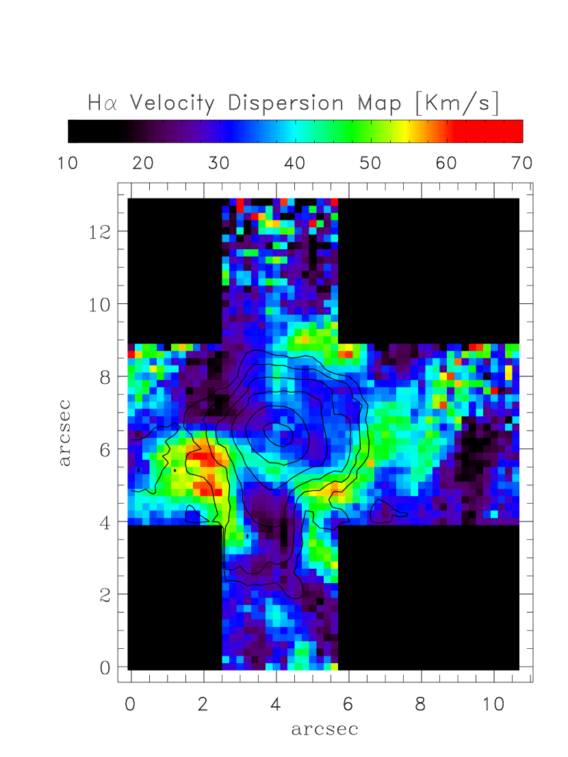
Figure 6: H$\alpha$ velocity dispersion map, corrected for instrumental and thermal broadening, of the inner region of II Zw 40. The contours represent 68, 20, 9, 5, 3.4 and 2.6% of the H$\alpha$ peak intensity. North is up and east is left.

The H$\alpha$ flux monochromatic map is a result of the emission line intensity measurements across the observed field. We fitted single Gaussians to the H$\alpha$ line profiles to derive their respective total fluxes, using the procedure discussed in Section 2. The H$\alpha$ monochromatic (total flux from the single Gaussian fit) contour map is presented superposed on the velocity dispersion and radial velocity maps (Figures 6 and 7) in six contours levels (68, 20, 9, 5, 3.4 and 2.6% of the peak intensity). The overall H$\alpha$ distribution in the synthetic map obtained from GMOS/IFU agrees very well with the narrow band H$\alpha$ image from ACS/HST at higher resolution (Figure 1). In the HST’s image it is possible to clearly resolve the two inner knots (A and B), the cavities formed by low H$\alpha$ emission maybe associated with superbubbles, and also some filaments. A synthetic red continuum image from our IFU data, shown here only in two contours in Figure 4, also reveals the two inner knots, separated by projected distance of 1.6$\arcsec$ ($\sim$ 90 pc). However, the Northern knot (A) is responsible for virtually all the ionizing luminosity in the core of II Zw 40 (Vanzi et al., 2008).

The starburst region revealed in II Zw 40, from the morphological point of view, is also very similar to the largest and extensively studied counterparts in the Local Group, such as 30 Dor, NGC 588 and NGC 604, showing complex kinematic features, along with filamentary structure, shells, and cavities, suggesting a common physical cause (Tenorio-Tagle et al., 2006). The similarities of the properties of the ISM in GHiiRs and HiiGs were first investigated through empirical relations of integrated physical parameters (Melnick et al., 1987, 1988), particularly the fact that both exhibit supersonic motions of the warm interstellar medium. A more detailed analysis of spatially resolved properties of these structures will help us understand the interplay between the massive cluster formation and evolution with its surrounding interstellar medium on scales of tens to hundreds of parsec.

3.4 The H$\alpha$ Velocity Dispersion and Radial Velocity Maps

The velocity dispersion map is presented in Figure 6, with H$\alpha$ intensity contours superposed. The region corresponding to the brightest knot (inner 50 pc) presents a low to intermediate $\sigma$ value (25-35  $\hbox{km}\thinspace\hbox{s}^{-1}$). There are, at least, three well defined high dispersion (45-65 km s^-1) regions $\sim$100 pc from the brightest knot. An almost constant velocity dispersion field ($\leq$ 35  $\hbox{km}\thinspace\hbox{s}^{-1}$), which contains most H$\alpha$ contour levels, is present in a region with 100$\times$100 pc² at NW of the brightest knot. At least two regions of low velocity dispersion (15-25  $\hbox{km}\thinspace\hbox{s}^{-1}$) are also found in the field, strikingly in between regions of high dispersion. A third low dispersion region is seen at extreme West, 300 pc far from the core, but we preferred to discard this from the analysis due to its low S/N.

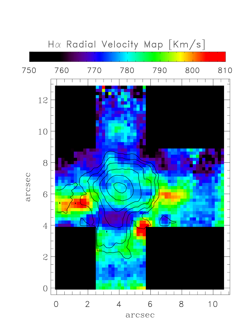
Figure 7: H$\alpha$ radial velocity map. The contours represent 68, 20, 9, 5, 3.4 and 2.6% of the H$\alpha$ peak intensity. The recession radial velocity is not corrected by the heliocentric motion. North is up and east is left.

The observed H$\alpha$ radial velocity map is shown in Figure 7. There is no sign of an overall rotation in the main starburst region of II Zw 40 ( 500$\times$500 pc²). On the other hand, discrete regions can reach high values of radial velocity, suggesting local expanding motions, although the total velocity range does not exceed 60  $\hbox{km}\thinspace\hbox{s}^{-1}$.

3.5 $Intensity$-$\sigma$ and $Intensity$-$Velocity$ Diagrams

An efficient method to identify kinematic features in GHiiRs, detect the massive clusters, their effect on the ISM, and their star formation rates, is by the analysis of the $Intensity$-$\sigma$ ($I$-$\sigma$) and $Intensity$-$Velocity$ ($I$-$V$) diagrams (Muñoz-Tuñón et al., 1996; Yang et al., 1996; Martínez-Delgado et al., 2007).

We present, in Appendix A, a schematic illustration of these diagrams, and a brief description of how they were previously interpreted by Muñoz-Tuñón et al. (1996). We also extend the analysis of these diagrams, including $V$-$\sigma$, to bring additional insight to the observed bulk motions.

In Figure 8 (left panel) we show the $I$-$\sigma$ plot for the whole observed field. The plot for II Zw 40 shows exactly the same basic features found in previous work on GHiiRs (Muñoz-Tuñón et al., 1996; Yang et al., 1996). In general low intensity regions have the highest $\sigma$ values while the range of $\sigma$ values decreases for high intensity regions. In the case of II Zw 40, there is a horizontal band defining a lower limit of $\sigma_{0}$ $\simeq$ 25 km s^-1 for regions brighter than 4000 counts (log F = 3.6). The horizontal line in the $I$-$\sigma$ plot shows the velocity dispersion of 33.5 km s^-1 derived from the integrated line profile with the 2.7$\arcsec$ aperture (Figure 5 left panel). It is a characteristic value for II Zw 40 found in all intensity regions. The inclined bands identified by Muñoz-Tuñón et al. (1996) are also identified in the plot. High velocity dispersions reach peaks of 65 km s^-1 in low intensity regions. As we will show in the next section, two inclined bands in this plot are superposed in the range 2.6 $<$ log F $<$ 3.1.

Some characteristic line profiles are also shown in Figure 8 (left panel). These are individual pixel profiles exemplifying the variety of shapes observed in different regions. Profiles (a) and (b) are the most asymmetric profiles observed. They originate close to the center of the two regions of high dispersion at SE and at SW of the brightest knot, respectively (see Figure 6). They are clearly double-peak profiles, consistent with expanding motions. Profile (c) originates in the second brightest knot and shows a prominent red wing. Profile (d) originates in the brightest knot and profile (e) comes from the lowest dispersion region.

Figure 8 (center panel) presents the $I$-$V$ plot which shows the relative radial velocity variations. These motions are usually associated with the line broadening component named $\sigma_{rad}$. The physical mechanisms at play which produce these line centroid variations should be several, such as turbulence, winds, champagne flows, expanding bubbles or rotation, acting on stellar radius scales to hundreds of parsecs. However, the estimate of the contribution of these subcomponents is limited to the spatial and espectral resolution of the observations. For instance, in this work we chose to associate the action of the spatially resolved bubbles, producing the highest radial velocity variations, to the component $\sigma_{rad}$. The other mentioned mechanisms, however, should also contribute to produce the overall pattern in the $I$-$V$ plot. Another line broadening component named $\sigma_{shell}$ will be here associated with the unresolved expanding shells identified as responsible for an underlying broad component found in the most inner region and discussed in section 3.7. Therefore, the position-to-position motions found in Figure 8 (center panel) contribute to the total broadening of an integrated line profile of the whole region. We do not intend to quantify precisely the contributions of the broadening components from the diagnostic diagrams. In the case of II Zw 40, the radial velocity differences are not higher than 15 km s^-1 in the brightest central region, and the highest differences are concentrated in low H$\alpha$ intensity regions. We found that the discrete tails toward high intensity values shown in Figure 8 (center panel) are associated with the presence of knot A (main tail) and B with a relative radial velocity of $\sim$ -13 km s^-1.

Figure 8 (right panel) shows the $V$-$\sigma$ plot. In the case of II Zw 40, it suggests that the overall motions in the star forming region are primarily random, instead of dominated by systematic line of sight motions. For instance, if one was observing a highly collimated outflow toward the line of sight, as a champagne flow, one should expect to see a trend in this diagram. Broad profiles from the low density regions should be found blueshifted, while narrow profiles from high density regions should be found redshifted, producing a pattern such as a narrow band with negative slope, not found for the whole region in Figure 8 (right panel). On other hand, the most important result shown by this diagram is that low $\sigma$ (15-25  $\hbox{km}\thinspace\hbox{s}^{-1}$) regions have small radial velocity variations, suggesting that they are close to the rest frame of the galaxy. This is the first indication that these regions may be unperturbed by massive stellar evolution.

We will try to associate the morphological features observed in the H$\alpha$ flux , velocity and dispersion maps with the features from these diagnostic diagrams by choosing individual regions for a more detailed analysis below.

3.6 The Kinematics of Individual Regions Revealed by Diagnostic Diagrams

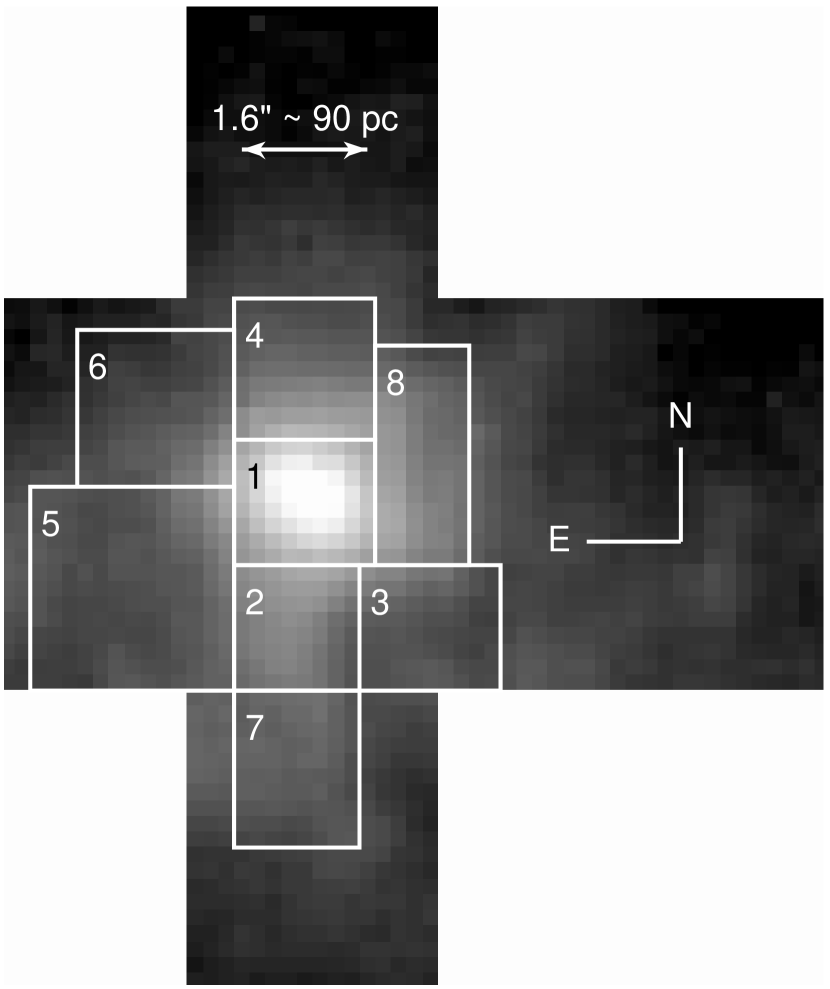
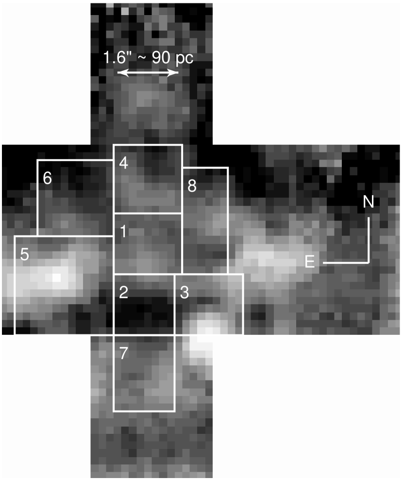
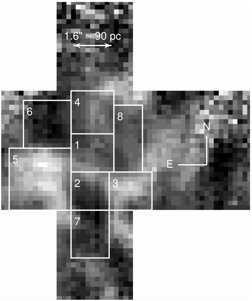
Figure 9: H$\alpha$ emission map (left), radial velocity map (center) and velocity dispersion map (right). The eight regions defined are drawn on each map.

The patterns shown in $I$-$\sigma$, $I$-$V$ and $V$-$\sigma$ plots (Figure 8) re-display many of the features that can be observed in the maps (Figure 6 and Figure 7). We wish to evaluate the contribution of individual features to the integrated H$\alpha$ line profile of II Zw 40 using the kinematic diagnostic diagrams. For this purpose, we defined eight regions with reliably measured $\sigma$ and radial velocity. The choice of regions was arbitrary, but motivated by different peculiarities noted in the H$\alpha$ flux, radial velocity and velocity dispersion maps. The chosen regions are superposed on these maps in Figure 9.

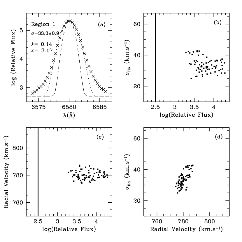
Figure 10: The panel present the four boxes discussed in the text for each region. The dashed line in box (1a) represents the instrumental profile (FWHM = 1.5Å). The dotted lines in all boxes 1 represent the single Gaussian fits to the integrated profiles. Note that in linear-logarithmic axes a Gaussian takes the form of a parabola. The region number and the $\sigma$ value derived are shown in the boxes (a). $I$-$\sigma$, $V$-$\sigma$ and $V$-$\sigma$ for each region are presented by boxes (b), (c) and (d), respectively. The vertical solid line in boxes (b) and (c) at log(Relative Flux) = 2.5 represent the estimated minimum line flux to well measure a single line profile.

For each chosen region, we have plotted a set of four graphs. These graphs are presented in Figure 10 in blocks of four boxes: (a) an integrated profile over the region in linear-logarithmic axes, where we also show the region number, the derived $\sigma$ value, and the estimated skewness $\xi$ and kurtosis $\kappa$ of each integrated profile, (b) $I$-$\sigma$, (c) $I$-$V$, and (d) the $V$-$\sigma$ plot. The vertical solid line in plots (b) and (c) shows our confidence limit in flux as described in Section 2. All references to the boxes in this section refer to Figure 10, where we quote the region number and the corresponding box letter, i.e. box (1a) means plot (a) of Region 1 in Figure 10. The results of the analysis of the emission line shapes through $\xi$ and $\kappa$ estimates for each region will be presented in Section 3.7. A brief description of each region follows:

Region 1 was defined to cover the main and brightest H$\alpha$ knot (knot A) as shown by the H$\alpha$ map (Figure 9 left). It covers an area of 1.8$\arcsec$ $\times$ 1.6$\arcsec$ (equivalent to 100 pc $\times$ 90 pc). The resultant integrated profile of Region 1 is shown in box (1a), where the dashed and dotted lines represent the instrumental profile and the Gaussian fit, respectively. The $\sigma$ derived for Region 1 was 33.3 km s^-1 which agrees with the value derived from our IFU simulated and FEROS spectra for a larger aperture (see Figure 5). Box (1b) shows that there is a well defined lower $\sigma_{0}$ value slightly above 25 km s^-1 and no high $\sigma$ variations. Radial velocity variations found in box (1c) indicates that the gas in Region 1 expands at $<$ 15 km s^-1. Since the points in box (1c) are within $\sim$ 7.5 km s^-1 from the average recession velocity, it is likely that the rms radial velocity variation contributes to an equivalent FWHM of $\sim$ 15 km s^-1 or $\sigma$ $\sim$ 6.5 km s^-1 (see Appendix A). Radial velocity variations between individual pixels in Region 1, therefore, do not contribute significantly to explain the total 33 km s^-1 velocity dispersion. At this spatial resolution only large scale radial velocity variations can be identified, and only these will be analyzed here ($\sim$ 50 pc). Box (1d) shows that most points are clustered with no apparent correlation between V and $\sigma$. We found that random motions are dominant in Region 1, instead of line of sight motions.

Region 2 was defined to cover the second brightest knot (knot B), south of Region 1. Region 2 covers an area equivalent to 90 pc $\times$ 90 pc. Box (2a) shows that, the integrated profile is the most asymmetric of all regions, showing a prominent red wing. This region is responsible for the red wing in the integrated profile obtained for II Zw 40 with FEROS, and also with our GMOS/IFU data (Figure 5). The reason for this asymmetry is that $\sigma$ reaches a local maximum in a few relative high intensity points (North of knot B) as shown by box (2b). Moreover, the same high intensity points, seen in box (2c), have the largest recession velocities, resulting in this observed red wing. As a consequence, box (2d) shows a strong correlation pattern (see Figure 13C). The radial velocity motions in Region 2 contribute twice as much to the integrate line width of the region as compared with Region 1 ($\sigma$ $\sim$ 13  $\hbox{km}\thinspace\hbox{s}^{-1}$). The gas in Region 2 has a relative line of sight motion with respect to the gas in Region 1 of roughly -13  $\hbox{km}\thinspace\hbox{s}^{-1}$. We found, however, two systematic components, one due to the relative radial motion between the two knots, and the other due to the expanding motion, as shown by the vertical band at log F $\sim$ 3.2 in box (2c) presenting an intermediate radial velocity variation.

Region 3 covers the SW high dispersion region. It covers an area of 1.8$\arcsec$ $\times$ 1.6$\arcsec$ (equivalent to 100 pc $\times$ 90 pc). The expected kinematic features due to the presence of an expanding shell are seen in all boxes for this region. Box (3a) shows a symmetric broad profile with $\sigma$ = 45.4  $\hbox{km}\thinspace\hbox{s}^{-1}$. This is actually the resulting smoothed profile obtained due to the contribution of unresolved asymmetries and multiple components as shown in one pixel profiles (a) and (b) of Figure 8 (left panel). Box (3b) clearly shows the inclined band indicating the presence of an expanding shell, possibly produced by an expanding bubble (see Figure 13A). Box (3c) confirms the expanding motion through the very high spread in radial velocity (see Figure 13B). The observed range of radial velocity, of about 20  $\hbox{km}\thinspace\hbox{s}^{-1}$  above and below the average recession velocity should underestimate the real radial component. This is in fact a limitation of fitting single Gaussians to the integrated profiles. From the line splitting in individual pixels in the center of the bubble we could measure a maximum $\Delta V$ $\sim$ 90 km s^-1 or a $V_{exp}$ $\sim$ 45 km s^-1. We estimated the radial velocity flow component to the integrated profile shown in box (3a) as FWHM $\sim$ 90 km s^-1 or $\sigma$ $\sim$ 38 km s^-1 (see Appendix A). Therefore, the expanding motion dominates the total broadening seen in the integrated profile of Region 3. The data points in Box (3d) show large scatter and there is not a significant trend in this plot, as seen in Region 2.

Region 4 covers an area of 1.8$\arcsec$ $\times$ 1.8$\arcsec$ (equivalent to 100 pc $\times$ 100 pc) and presents a field of intermediate $\sigma$ and H$\alpha$ intensity values, north of knot A. Region 4 presents many similarities with Region 1: similar $\sigma$ derived as shown in box (4a) and similar pattern in box (4b) showing low $\sigma$ variations and a lower limit $\sim$ 25  $\hbox{km}\thinspace\hbox{s}^{-1}$. The small radial velocity variations found in box (4c) and a concentrated velocity dispersion distribution in (4d) indicate that there is no significant systematic motions contributing to the total line broadening, which is dominated by random motions on scales smaller than the seeing of $\sim$20 pc.

Region 5 is one of the most interesting regions, and covers a large area of 2.6$\arcsec$ $\times$ 2.6$\arcsec$ (equivalent to 150 pc $\times$ 150 pc) SE of knot A. It presents some of the broadest profiles, and it is probably associated with an expanding shell (boxes 5a and 5b). Region 5 also presents high radial velocity spread (box 5c) of over 40  $\hbox{km}\thinspace\hbox{s}^{-1}$, although this may underestimate the real radial velocity component as argued above in the analysis of Region 3. Regions 3 and 5 show very similar patterns in all diagrams, suggeting that these patterns can be easily used as expanding shell diagnostics in GHiiRs. Despite their different sizes and morphologies the two shell regions have similar kinematic properties. Some double peak profiles seen in Region 5 are also consistent with a bubble expanding with a velocity of 45  $\hbox{km}\thinspace\hbox{s}^{-1}$, likely to be powered by supernovae and stellar driven winds. There is not a significant trend found in box (5d).

Region 6 was defined to cover a field containing the lowest velocity dispersion values. It covers an area of 2.0$\arcsec$ $\times$ 2.0$\arcsec$ (equivalent to 110 pc $\times$ 110 pc) North-East of Region 1. The observed $\sigma$ = 23.5  $\hbox{km}\thinspace\hbox{s}^{-1}$, as shown in box (6a), is the lowest value verified of all regions. Box (6b) also shows that a significant area presents $\sigma$ values lower than knot A, though they are still supersonic. Velocity variations are also very small as shown by box (6c). Box (6d) indicate primarily random motions. All plots suggest, therefore, that Region 6 represents a region where the mechanical energy input resulting from massive star evolution does not play a significant role to stir the gas up.

Region 7 presents a relatively low velocity dispersion field (box 7a). It covers an area of 1.6$\arcsec$ $\times$ 2.0$\arcsec$ (equivalent to 90 pc $\times$ 110 pc), South of knot B. It completes the sampling of a larger low-to-intermediate dispersion field covered partially by Region 2 (boxes 2b and 7b). Both regions are confined between the two high dispersion bubbles, Regions 3 and 5. The H$\alpha$ structure in Region 7 is associated with the extended emission to the South of both knots (see Figure 9 left panel). Box (7c) shows a weak correlation of $I$ and $V$ with fainter emission points moving away. However, no clear correlation between radial velocity and $\sigma$ is seen in box (7d).

Region 8 covers an area from W to NW of the knot A (equivalent to 70 pc $\times$ 160 pc) with a $\sigma$ = 32 km s^-1 (box 8a), similar to Region 1. It was defined to contain a field with almost constant velocity dispersion through a large range of intensities, which is shown by box (8b). The pattern formed in box (8b) is not an inclined band. Region 8 does not present high velocity variations, as shown by box (8c) and it is likely dominated by random motion inferred by the points concentrated in box (8d). The few higher dispersion points at low intensities seen in box (8b) and (8d) may be picking up a possible additional region of interest (i.e. shell) North of Region 8 (see Figure 9 right panel) which is not well mapped in our observations and is not included in the present analysis.

Our definitions of the regions favor the interpretation of the different patterns in $I$-$\sigma$ diagrams where kinematic features are easily identified. Thus, the patterns may be the result of different physical mechanisms. Something to have in mind here, is our spatial resolution which only permits us to identify kinematic features in scales of a tens of parsec and limited by our field size. The overall picture is that local systematic motions represent a dominant component to the observed line widths in regions 3 and 5 which are likely associated with resolved expanding shells due to the fact that we can observe line splitting directly. Although, masked by the use of single Gaussians, they leave a signature in the diagnostic diagrams. Region 1 presents a small range of intermediate $\sigma$ values which are also found in all the intensities of nebular emission across the whole extent of the star forming region. Region 2 is turbulent with some characteristics of flow motions. Regions 4, 7 and 8 show smooth turbulent fields. Wherever we cannot observe double peaked profiles in these regions, we cannot completely rule out a radial systematic component to the line width, possibly associated with unresolved shells, however random motions must dominate over expansion in these cases. Finally, relatively to the other regions, Region 6 seems to be slightly affected or even unperturbed by mechanical energy input provided by massive star evolution, presenting the lowest $\sigma$ values.

3.7 Making up the Integrated Velocity Profile from Individual Regions

Figure 11 shows the fully integrated line profile produced by combining all eight spectra for the regions presented in § 3.6, with a resulting $\sigma$ = 34.1  $\hbox{km}\thinspace\hbox{s}^{-1}$. Despite the complex medium-scale structures (50-100 pc) seen in the synthetic maps (Figures 6 and 7), mainly due to the presence of asymmetries and multiple components (e.g., profiles (a) and (b) of Figure 8 left panel), the fully integrated profile is quite smooth and symmetric.

An important result is that the velocity dispersion derived from a single Gaussian fit to the profile of Region 1 (Figure 10 box 1a) is virtually the same as those derived from the original FEROS spectrum with an aperture of 2.7″, and the simulated spectrum with the FEROS aperture on our GMOS/IFU data (Figure 5), and the fully integrated line profile (Figure 11). Region 1 represents 10% of the total area analyzed but 49% of the total H$\alpha$ flux in all eight regions. In contrast, Region 3 and 5, showing the broadest profiles, cover 33% of the total area analyzed but only contribute 14% to the total flux. Other regions, namely Region 6 and 7, covering 25% of the total area and showing the lowest $\sigma$ values only contributes 10% to the total H$\alpha$ flux. All the highest surface brightness regions, namely Region 1, 2, 4 and 8, show the common values $\sigma$ = 32-35 km s^-1 which characterize the global kinematics of the warm gas in II Zw 40’s dominant starburst region.

The aperture effect to derive the characteristic velocity dispersion of II Zw 40 is negligible if an integrated spectrum is taken with an aperture covering the brightest knot. As an example, Melnick et al. (1988) derived for II Zw 40 a $\sigma$ = 35.2$\pm$0.5 km s^-1 with a 6$\arcsec$ wide entrance slit aperture. From an observational point of view, this result is very positive. If the same is valid for most HiiGs and GHiiRs, as has been confirmed, the measured supersonic $\sigma$, introduced in the $L$-$\sigma$ relation, is little affected by the effects of SNRs and wind driven bubbles where the warm gas emission is faint, and where the integrated velocity dispersion is much higher than in the central core.

We computed the skewness, $\xi$, and the kurtosis, or flatness factor, $\kappa$, to quantify the shape of each profile and they are included in all boxes (a) of Figure 10. We warn that the quantitative results, especially for $\kappa$, are sensitive to the window of summation and the height of continuum. We defined a confident fixed window 6576-6584Å to compute the $\xi$ and $\kappa$ values, since broad wings are not well mapped for the faintest profiles. Relative differences between kurtosis values are more significant than their absolute values, which should in principle be comparable with a Gaussian profile ($\xi$=0, $\kappa$=3). We found that most profiles have peaked shape $\kappa$ $>$ 3 (leptokurtic). Region 3 and 5 are significantly more flattened than the others (platykurtic). The most asymmetric profiles identified by the highest $\mid\xi\mid$ are those of Region 2 and 6, which can be easily distinguished visually in liner-logarithmic plots in boxes (2a) and (6a) of Figure 10. We also estimated $\xi$ and $\kappa$ values for the fully integrated profile shown in Figure 11. We can see that not only the $\sigma$ but also $\xi$ and $\kappa$ values are virtually identical to those estimated from profile of Region 1 (Figure 10 box 1a).

Since the S/N in the wings of the profile from Region 1 is much higher than the others, we were able to measure across in a larger window (6574-6586Å) and estimate another pair of $\xi$ and $\kappa$ values for this profile, giving an idea of how sensitive the values of the higher order moments are. The estimated values derived in this spectral range are $\xi$=0.14 and $\kappa$=4.19, showing that the integrated profile in Region 1 is very peaked. This result indicates the presence of a broad but weaker component in the core of II Zw 40. Multicomponent Gaussian fits to the profile of Region 1 are shown in Figure 12. We used the PAN routine (Peak ANalysis; Dimeo (2002)) in IDL to fit two components to H$\alpha$ profile. We found a narrow component $\sigma_{n}$ = 29.4$\pm$0.6 km s^-1 which is not very different from $\sigma$ derived from a single fit $\sigma$ = 33.3$\pm$0.9 km s^-1. The broad component was estimated to be $\sigma_{b}$ = 73.2$\pm$1.0 km s^-1 and its flux corresponds 18% to the flux of the narrow component. We may speculate that the broad component is associated with unresolved wind-driven shells at the core of II Zw 40 where most of the young and massive stars concentrate.

4 Discussion

An important verification provided by the above results is that the H$\alpha$ kinematic features already found in Local Group’s GHiiRs are represented in the main starburst region of II Zw 40: a prototypical Hii galaxy at roughly 11.9 Mpc. In fact, one way to investigate the starburst phenomena on these galactic scales is to compare the main starburst region in II Zw 40 with the local GHiiRs studied by similar techniques.

Yang et al. (1996) found that virial motions and expanding shells contribute roughly equally to the velocity width of the integrated profile in NGC 604. Using the same methods, Muñoz-Tuñón et al. (1996) proposed an evolutionary scenario when they compared their results of NGC 604 with NGC 588. A simple model for an idealized homogeneous shell evolving in a uniform density medium suggests that younger and fast shells should have lower intensities and reach higher $\sigma$ values than older ones. Hence, the authors argue that NGC 604 appears to be younger than NGC 588 based on the inclined bands associated with shells, and identified in $I$-$\sigma$ plots. Furthermore, NGC 604 presents a well defined lower limit ($\sigma_{0}$ $\simeq$ 17 $\hbox{km}\thinspace\hbox{s}^{-1}$) in supersonic line width everywhere (horizontal band in $I$-$\sigma$ plot), while NGC 588 does not. A substantial fraction of NGC 588 presents line widths lower than the brightest region, including points showing subsonic $\sigma$ values. Melnick et al. (1999) suggest that it is also the case for 30 Dor. In the Cometary Stirring Model (CSM) framework, this difference can also be understood as an evolutionary effect. A young region keeps most of the supersonic motions communicated to the leftover gas via bow shocks by the winds of low-mass stars during its early stage. As massive stars evolve, ejecting mechanical energy into the ISM, through stellar winds and supernova events, they produce shells that expand beyond the core. Shells will be destroyed by random motions of the background neighboring gas and slow down, resulting in $\sigma$ even below the bright region (Tenorio-Tagle et al., 1993; Muñoz-Tuñón et al., 1996). The main point in this scenario is that the dominant line-broadening mechanism in young GHiiRs is gravity, while tuburlence by wind-driven shells and supernovae dominate in older ones.

More recently, Martínez-Delgado et al. (2007) have shown that the morphological features observed in their analysis of three-dimensional spectroscopic data of three blue compact galaxies (Mrk 324, Mrk 370, and III Zw 102), especially those in the $\sigma$ $versus$ $I_{peak}$ diagram, look similar to the ones found in GHiiRs, with a supersonic horizontal band that extends over a large range of intensities, and inclined bands that reach high $\sigma$ values at low intensity arising from large volumes surrounding the central knots. In a similar study to our own, using similar technique with Gemini GMOS/IFU, Westmoquette et al. (2007a, b) looked at the properties of a young star cluster and its environment in the dwarf irregular starburst galaxy NGC 1569. Despite the fact that they decompose the profiles rather than fit a single Gaussian, the narrow components of their profiles show all properties found in these other studies including ours, namely that, it is most likely explained by a convolution of the stirring effects of massive star evolution and gravitational motions. In addition, they found that the observed lower limit ($\sigma_{0}$ $\simeq$ 12 km s^-1) of the narrow component is in agreement with $\sigma_{virial}=\sqrt{GM/R}$.

Here, we wish to test the hypothesis that the dominant broadening mechanism of the H$\alpha$ line in the core of II Zw 40 is gravity.

As shown in Figure 8 (left panel), II Zw 40 presents the lowest $\sigma$ values ($\sigma$ $\sim$ 20 km s^-1) in regions with faint H$\alpha$ emission. Here we identify Region 6 as the most significant contributor to this low $\sigma$ (see Figure 10 box 6b), which appears to present dominantly random motions, through its diagnostic diagrams. In addition, Region 6 does not seem to be affected by the neighboring superbubble of Region 5. Therefore, this region may still retain the kinematic information of the pre-existing underlying turbulent velocity field. The velocity dispersion values derived in Region 6 should not be associated with the internal velocity dispersion of individual dense molecular cloud cores or clumps (typically less than a few  $\hbox{km}\thinspace\hbox{s}^{-1}$), where individual or groups of massive stars form, but instead, they may be the result of the large scale turbulent motions of the parent complex of diffuse molecular clouds, which gave rise to the present episode of violent star formation. Some of these clouds will form stars in short local dynamical times, while others, though dense, may not form stars. We do not intend to discuss any detailed model, but simply try to envisage a viable scenario for our conjecture of an overall underlying velocity component. Massive star clusters will form in much denser fragments (clumps or cores) of the molecular clouds whose properties are not assessed by our observations, and require density tracers (e.g. HCN) with high spatial resolution radio observations. Though, these clumps must also have relative velocities stirring up the ISM under the influence of the common gravitational potential due to the complex of stars, and gas, and possibly dark matter. The ¹²CO (J= 1 $\rightarrow$ 0) traces the diffuse molecular cloud on hundreds of parsec scales. The measured CO line width of a region encompassing the entire ionized region in II Zw 40 is $\Delta$V = 42 km s^-1 or $\sigma$ $\sim$ 18 km s^-1 (Tacconi & Young, 1987), somewhat comparable to the low $\sigma$ in the ionized gas. However, these motions seem to be completely detached from the global HI velocity distribution which extends up to 5 arcmin ($\sim$ 6 Kpc) in the direction of the southern and northern tails (van Zee et al., 1998; Brinks & Klein, 1988), where the line width is W${}_{50}\sim$ 120 km s^-1 ($\sigma\sim$ 50 km s^-1) and has a strong contribution by the large scale rotation pattern of the galaxy on these scales.

The large resolved supperbubble in Region 5 is very well delimited in $\sigma$ and intensity maps and may not have slowed down sufficiently to be disrupted. Moreover, Region 3 also presents a well defined bubble in $\sigma$ and intensity maps, which is seen as an inclined band in the diagnostic plot. Despite being smaller than the bubble in Region 5, they both show similar profile shapes, expansion velocities $V_{exp}$ $\sim$ 45  $\hbox{km}\thinspace\hbox{s}^{-1}$, and integrated velocity dispersions $\sigma$ $\sim$ 45  $\hbox{km}\thinspace\hbox{s}^{-1}$, possibly indicating similar evolutionary phase and associated with the age of knot B.

Although II Zw 40 contrasts slightly with a simple scenario for a GHiiR, in the sense that it may suffer from the composite effects resulting from the evolution of multiple stellar clusters, we can say that in the CSM context, the GHiiR in II Zw 40 is kinematically young. Some superbubbles are evolving within the core, though it does not present a constant $\sigma$ or only “well-behaved” Gaussian emission lines (Muñoz-Tuñón et al., 1995, 1996). However, the presence of surrounding regions showing lower $\sigma$ than the core in II Zw 40 is a sign of youth. There are still unperturbed regions preserving kinematic information of the parent cloud under the dominant influence of the galaxy’s gravitational potential, ionized by diffuse UV radiation. In consonance with our conclusions, many studies about this galaxy indicate the presence of a very young starburst in its brightest region, as mentioned in the introduction.

An important resolution bias must be of concern here in order to test our hypothesis. Melnick et al. (1999) show that the supersonic integrated line profile in 30 Dor is actually due to a superposition of discrete number of clouds, small shells and filaments which are resolved on subparsec scales. In these scales, strong winds of WR, O and B stars might be responsible for stirring up the gas around the dominant young cluster, imposing a turbulent motion higher than the one predicted only by the gravitational potential. The presence of a significant number of the very young stars in the core should be responsible partially for the difference between the $\sigma$ found in Region 1 and that one found in Region 6. In fact, we found evidence of a broad component $\sigma_{b}$ $\sim$ 73 km s^-1 in Region 1, responsible for the large wings in the integrated profile, which may be associated with unresolved inner shells. However, its contribution to the integrated profile is very small, since only 18% of the total H$\alpha$ flux in Region 1 comes from this component.

We can now sum up the main reasoning so far. A common framework assumes that the observed velocity dispersion ($\sigma_{obs}$) is mainly given by the contributions of gravity ($\sigma_{grav}$), thermal broadening ($\sigma_{th}$), multiple unresolved expanding shells ($\sigma_{shell}$) and systematic radial motions ($\sigma_{rad}$). Here we consider $\sigma_{rad}$ as being the sum of several phenomena such as SN, expanding bubbles, champagne flows, relative motions between discrete clusters providing large scale shear, turbulence and rotation, which cause position-to-position radial velocity variations and, in extreme cases, line splitting. We detected and identified $\sigma_{shell}$ only in the core, i.e. Region 1, as the weak broad component, but possibly present with different weights in the whole nebula. Indeed, we found that most profiles have peaked shape indicating the presence of faint wings or broad components, with the exception of those found in regions of bubbles, i.e. Region 3 and 5. Once corrected for the instrumental profile, the observed velocity dispersion of a GHiiR or discrete regions inside them is therefore given by

$$\sigma_{obs}=\sqrt{\sigma_{grav}^{2}+\sigma_{shell}^{2}+\sigma_{th}^{2}+\sigma_{rad}^{2}}$$

(Melnick et al., 1999). We fixed the thermal broadening as $\sigma_{th}$ = 9.1 km s^-1 due to the gas electron temperature for hydrogen at 10⁴K, causing no significant systematic error in our results. The radial velocity variations on scales larger than 50 pc can be identified here. It varies from few km s^-1 in regions such Region 1, $\sigma_{rad}$ $\sim$ 6.5 km s^-1, to $\sigma_{rad}$ $\sim$ 38 km s^-1 in Regions 3 and 5 as inferred from line splitting in the center of bubbles. Region 6 seems to be “free from shells”, and it can be a good probe of $\sigma_{grav}$ $\sim$ 20-25 km s^-1, posing a lower limit of velocity dispersion in II Zw 40. In fact, these values are not very different from the narrow component found in Region 1, $\sigma_{n}$ $\sim$ 29 km s^-1, and the lower limit $\sigma_{0}$ $\sim$ 25 km s^-1 in the $I-\sigma$ diagnostic diagram. If indeed, the $\sigma$ measured in Region 6, is unaffected by stellar evolution, and the narrow component of the Gaussian fit to the profile of Region 1 gives the same low value of $\sigma$, and additionally the low limit of overall measured $\sigma$ is probing the same physical mechanism, we may suggest a common dominant line broadening cause. Gravity provides the continuous underlying source of stirring the ISM over the whole star-forming region. However, the characteristic $\sigma$ = 32-35 km s^-1 found over the whole starburst region of II Zw 40 and derived from a single Gaussian fit should be the result of combined sources, of the dominant action of gravity, unresolved multiple expanding shells and systematic radial motions.

5 Summary

The three-dimensional spectroscopic analysis of II Zw 40, using Gemini-North GMOS/IFU, yield insights into several astrophysical questions about the structure and evolution of starburst regions, specially those associated with the birth of super star clusters and their impact on the ISM. The kinematics of the warm gas inferred from line profiles of emission lines, such as H$\alpha$, imposes constraints on the theoretical models of star formation and on feedback of stellar evolution on the ISM. We have analyzed the kinematic properties of the ionized gas in II Zw 40 using diagnostic diagrams and individual region description. A summary of the main conclusions follows:

• Electron densities in the inner starburst region range from $5\times 10^{2}$ to $1.4\times 10^{3}$ cm^-3, somewhat higher than the common low density regime for Hii regions of 10² cm^-3. Its spatial distribution is not constant and shows a clear decline (compatible with an r^1/4 law) with a peak coincident with the H$\alpha$ line emission peak.

• Oxygen abundance as inferred by the N2 calibrator in the inner 100 $\times$ 100 pc² ranges from 12+log(O/H) = 7.8 to 8.4, showing lower values 12+log(O/H) = 7.85 associated with the dominant site of star formation, namely knot A.

• The aperture effect to infer the characteristic velocity dispersion $\sigma$ = 34 km s^-1 of II Zw 40, derived from a single Gaussian fit, is negligible. All shape properties ($\sigma$, $\xi$ and $\kappa$) of a fully integrated profile are virtually the same as those found in the profile of the brightest region.

• The diagnostic diagrams of $I$ $versus$ $\sigma$, $I$ $versus$ $V$, and additionally $\sigma$ $versus$ $V$ are powerful tools to identify the origin of internal motions in GHiiRs and also in HiiGs.

• We found regions where stellar evolution does not seem to play a significant role stirring the gas up, and should reveal the kinematic signature of the proto-cloud that gave rise to the present starburst. In the case of II Zw 40, Region 6 North-East of the main knot poses a lower limit of $\sim$ 23  $\hbox{km}\thinspace\hbox{s}^{-1}$  to the global velocity dispersion in the galaxy, which should provide a good estimate of $\sigma_{grav}$.

• Despite the different sizes and morphologies, the two large shells found in Region 3 and 5 have the same kinematic properties, with very similar patterns in all diagnostic diagrams. Both regions have smoothed integrated line profiles with $\sigma$ $\sim$ 45  $\hbox{km}\thinspace\hbox{s}^{-1}$  and they seem to expand at $V_{exp}$ $\sim$ 45  $\hbox{km}\thinspace\hbox{s}^{-1}$, contributing significantly with $\sigma_{rad}$ $\sim$ 38  $\hbox{km}\thinspace\hbox{s}^{-1}$  to the total width of their integrated profile.

• The inner 50 pc and brightest region of II Zw 40 seems to be kinematically very young, where gravity seems to play an important role. Part of the difference found between $\sigma$ $\sim$ 33 km s^-1 in the core and 23  $\hbox{km}\thinspace\hbox{s}^{-1}$  found in Region 6 is possibly associated with a weak broad component and a small systematic radial velocity flow component $\sigma_{rad}$. The broad component should be associated with $\sigma_{shell}$ originated from multiple unresolved shells provided by stellar winds of WR and OB stars acting on few or subparsec scales.

• The kinematic features in II Zw 40 are all remarkably similar to the ones found in supersonic GHiiRs in irregular and other star forming galaxies powered by massive star and stellar cluster formation and evolution, suggesting that these starbursts in HII galaxies are their scaled up versions on galactic scales.

Finally, the core supersonic $\sigma$ is the one producing the Luminosity-$\sigma$ relation observed in GHiiRs and HiiGs. This component can be derived by simply measuring the integrated line profiles by fitting a single Gaussian on the brightest knot of the starburst, regardless of aperture size. However, we must further investigate how these derived motions precisely relate to the underlying mass distribution before we can derive absolute total galactic masses. We must also investigate, with a statistically significant sample, the possible evolutionary effects of the starburst on the observed relations, and how they can be parametrized for the use as a powerful extragalactic distance estimator applied to high redshifts.

Appendix A Interpreting the Diagnostic Diagrams

It is convenient to emphasize the meaning of some patterns formed by the point distributions in the different diagnostic diagrams of Figure 8. These patterns are the graphical representation of the kinematic signatures observed in the 2D flux, velocity and dispersion maps. The following description is valid for the methodology of fitting only single Gaussians to the emission line profiles and its limitation is emphasized when necessary. However, it is a very powerful tool for kinematic analysis provided by data cubes. Three typical patterns are of particular interest, and they are sketched in diagrams (A), (B) and (C) of Figure 13.

Figure 13A shows the pattern known as the inclined band in the $I$-$\sigma$ diagram, previously identified by Muñoz-Tuñón et al. (1996). The authors propose that this pattern should be the result of an ideal shell evolving in the ISM. Their scenario allows the interpretation of this diagram as a diagnosis for the evolutionary state of the GHiiRs. The points defining the vertexes of the triangle should correspond to the three parts of the shell: center, inner edge and outer edge (see their Fig. 3). The velocity dispersion in the center reaches the maximum value, while the minimum value occurs in the outer edge. The inner edge presents higher intensity and higher velocity dispersion than the outer edge. Assuming that the pattern drawn in the Figure 13A represents a young shell, as it ages, $\sigma$ at the center becomes gradually lower, as well as the difference between the intensity at the center and at the inner edge. Then, the whole figure shifts down, and the upper angle becomes smaller. Furthermore, in their scenario, older shells should present higher intensities than young ones, and should be mapped at right of the young ones in the diagram.

Figure 13B shows a vertical band pattern in $I$-$V$ diagram. This pattern indicates the contribution of resolved systematic radial movements. Abrupt velocity variations in a short intensity range should indicate a local expansion of the gas. It is expected that regions which present the inclined band pattern in the $I$-$\sigma$ diagram also present a well defined vertical band pattern in $I$-$V$ diagram. In general, any vertical variations ($\Delta V$) can be used to quantify the component due to expanding motions in a region. We used the approximation FWHM${}_{rad}\sim$ $\Delta V$ to infer the broadening component due to radial velocity variations ($\sigma_{rad}$) for regions with almost constant $\sigma$ values and nearly Gaussian emission line profiles. However, if the emission profiles are not well represented by single Gaussians, $\Delta V$ measured in $I$-$V$ plot should underestimate the real component due to systematic radial expansion. As an alternative, one might try to measure the line splitting from the most asymmetric or double peaked profile, in order to better estimate $\Delta V$ from two centroids.

Figure 13C shows a correlation between $V$ and $\sigma$. This pattern indicates systematic motion with a significant component in the line of sight. The pattern drawn indicates differentiated group behavior: in this case, gas with relatively high $\sigma$ is moving away from the observer. Although we have drawn the pattern with a positive slope, a region with the same systematic motions could be identified in a negative slope pattern. Such dependence should be expected in the presence of relative motions between distinct clouds of ionized gas with different internal properties. Champagne flows should reproduce the pattern like the one shown in Figure 13C (see $\S$ IIIc in Skillman & Balick (1984)). The simplest pattern would be the random distribution of the points in the plane $V$-$\sigma$, indicating no dependence between the variables. In this latter case, it may represent isotropic expansion or turbulence, but with no privileged direction.

Figure 2: Single pixel spectrum on the bright core centered on knot A. The labels show most of the emission lines present on our spectrum from 6250Å to 7400Å. The y axis has been cut to illustrate the relative intensity of the lines, in particular the much larger intensity of the H$\alpha$ line which is used in this work.

Figure 3: Electron density distribution in the central field, derived from an azimuthal fit to isointensities of the ratio of the sulfur line ([SII]$\lambda\lambda$ 6717,6731) maps. The solid line is a r^1/4 linear fit to the data. The dotted line is a Gaussian profile to represent the approximate seeing during this observation.

Figure 5: Line profiles derived with GMOS/IFU (left) and FEROS (right) data. The dashed lines represent the respective instrumental profiles (FWHM = 1.5Å for the GMOS and FWHM = 0.13Å for the FEROS). The dotted lines represent the single Gaussian fits. The velocity dispersions values derived are shown in the boxes.

Figure 8: $I$-$\sigma$ (left), $I$-$V$ (center) and $V$-$\sigma$ (right) plots for the whole region observed in II Zw 40 as described in the text. The solid horizontal line in $I$-$\sigma$ plot represents the $\sigma$ value for the inner core (D = 2.7$\arcsec$). Characteristic individual pixel line profiles are shown in the left panel from (a) to (e). Dashed lines represent the single Gaussian fits and the dotted line under profile (d) is the instrumental profile. The vertical solid line at log(Relative Flux) = 2.5 represent the estimated minimum line flux to well measure a single line profile. All points with log(Relative Flux) $<$ 2.5 are not shown in $V$-$\sigma$ plot.

Figure 10: Continued. Only Region 6 presentS points with log(Relative Flux) $<$ 2.5 and they are not shown in box 6b.

Figure 11: The fully integrated profile summing all eight regions analyzed in section 3.6. The dotted line represent the single Gaussian fit to the profile.

Figure 12: The integrated profile of Region 1 (same in Figure 10 box 1a) plotted in linear axes. The profile is well fitted by two Gaussians and the profiles are plotted. The dashed line represents the narrow component $\sigma_{n}$, whereas the dotted line represents the broad component $\sigma_{b}$. The solid line shows the resultant profile.

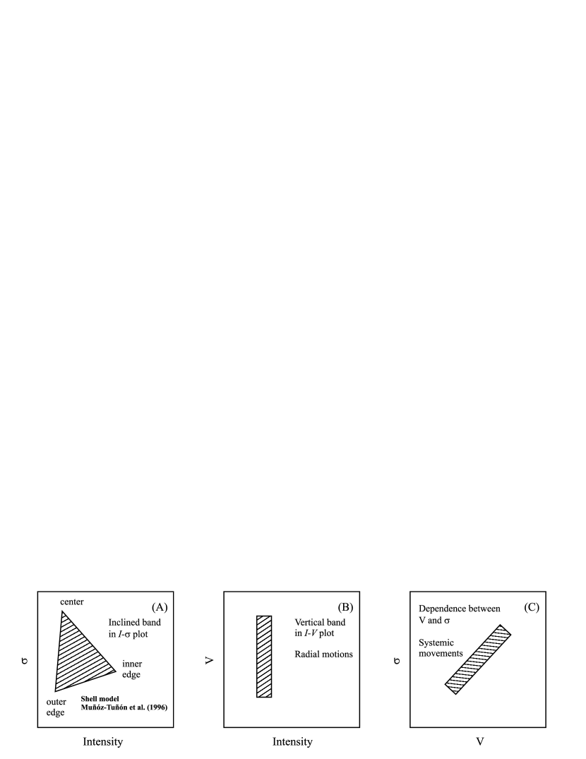
Figure 13: Schematic diagrams showing idealized patterns formed by the distribution of points discussed in the text.

References

- Baldwin et al. (1982) Baldwin, J. A., Spinrad, H., & Terlevich, R. 1982, MNRAS, 198, 535
- Beck et al. (2002) Beck, S.C., Turner, J.L., Langland-Shula, L.E., Meier, D.S., Crosthwaite, L.P., Gorjian, V. 2002, AJ, 124, 2516
- Bosch et al. (2002) Bosch, G., Terlevich, E., & Terlevich, R. 2002, MNRAS, 329, 481
- Boulesteix (1999) Boulesteix J. ADHOC User’s Manual http://www-obs.cnrs-mrs.fr/adhoc/adhoc.html
- Brinks & Klein (1988) Brinks, E., & Klein, U. 1988, MNRAS, 231, 63
- Castellanos et al. (2002) Castellanos, M., Díaz, A. I. & Terlevich, E. 2002, MNRAS, 329, 315
- Chu & Kennicutt (1994) Chu, Y.-H., & Kennicutt, Jr., R. C. 1994, ApJ, 425, 720
- Cumming et al. (2008) Cumming, R. J., Fathi, K., Ostlin, G., Marquart, T., Márquez, I., Masegosa, J., Bergvall, N., Amram, P., 2008, A&A, 479,725
- Dimeo (2002) Dimeo, R. 2005, PAN User Guide, ftp://ftp.ncnr.nist.gov/pub/staff/dimeo/pandoc.pdf
- Denicoló et al. (2002) Denicoló, G., Terlevich, R. & Terlevich, E., 2002, MNRAS, 330, 69
- Dopita & Sutherland (2003) Dopita, M.E. & Sutherland, R.S.,in “Astrophysics of the Diffuse Universe”, 2003, Springer-Verlag Berlin Heidelberg New York
- Dyson (1979) Dyson, J. E. 1979, A&A, 73, 132
- Fuentes-Masip et al. (2000) Fuentes-Masip, O., Muñóz-Tuñón, C., Castañeda, H. O., & Tenorio-Tagle, G. 2000, AJ, 120, 752
- Hibbard & Milhos (1995) Hibbard, J. E., & Mihos, J. C. 1995, AJ, 110, 140
- Kaufer et al. (1999) Kaufer, A., Stahl, O., Tubbesing, S., Norregaard, P., Avila, G., Francois, P., Pasquini,L. & Pizzella, A. 1999, The Messenger 95, 8
- Kehrig et al. (2004) Kehrig, C., Telles, E., & Cuisinier, F. 2004, AJ, 128, 1141
- Kunth & Sargent (1981) Kunth, D., & Sargent, W. L. W. 1981, A&A, 101, L5
- Maíz-Apellániz et al. (1999) Maíz-Apellániz, J., Muñoz-Tuñón, C., Tenorio-Tagle, G., & Mas-Hesse, J. M. 1999 A&A, 343, 64
- Martínez-Delgado et al. (2007) Martínez-Delgado, I., Tenorio-Tagle, G., Muñoz-Tuñón, C., Moiseev, A., Cairós, L. M., 2007, AJ, 133, 2892
- Melnick (1977) Melnick, J. 1977, ApJ, 213, 15
- Melnick et al. (1987) Melnick, J., Moles, M., Terlevich, R., & Garcia-Pelayo, J.-M. 1987, MNRAS, 226, 849
- Melnick et al. (1988) Melnick, J., Terlevich, R., & Moles, M. 1988, MNRAS, 235, 297
- Melnick et al. (1999) Melnick, J., Tenorio-Tagle, G., & Terlevich, R. 1999, MNRAS, 302, 677
- Miesch & Scalo (1995) Miesch,M.S. & Scalo, J.M. 1995, ApJ, 450, L27
- Münch (1958) Münch, G. 1958, Cosmical Gas Dynamics, Proceedings from IAU Symposium no. 8. Edited by Johannes Martinus Burgers and Richard Nelson Thomas. International Astronomical Union. Symposium no. 8, p. 1035
- Muñoz-Tuñón et al. (1995) Muñoz-Tuñón, C., Gavryusev, V., & Castañeda, H. O. 1995, AJ, 110, 1630
- Muñoz-Tuñón et al. (1996) Muñoz-Tuñón, C., Tenorio-Tagle, G., Castañeda, H. O., & Terlevich, R. 1996, AJ, 112, 1636
- Östlin et al. (2004) Östlin, G., Cumming, R. J., Amram, P., Bergvall, N., Kunth, D., Márquez, I., Masegosa, J., Zackrisson, E., 2004, A&A, 419, L43
- Pelupessy et al. (2004) Pelupessy, F.I., van der Werf, P.P & Icke, V., 2004, A&A, 422, 55
- Rozas et al. (2006) Rozas, M., Richer, M. G., López, J.A., Relaño, M., & Beckman, J. E. 2006, A&A, 455, 539
- Roy et al. (1991) Roy, J.-R., Boulesteix, J., Joncas, G., & Grundseth, B. 1991, ApJ, 367, 141
- Sargent & Searle (1970) Sargent, W. L. W. & Searle, L. 1970, ApJ, 162, 155
- Searle & Sargent (1972) Searle, L., & Sargent, W. L. 1972, ApJ, 173, 25
- Skillman & Balick (1984) Skillman, E. D., & Balick, B. 1984, ApJ, 280, 580
- Smith & Weedman (1970a) Smith, M. G., & Weedman, D. W. 1970a, ApJ, 161, 33
- Smith & Weedman (1970b) Smith, M. G., & Weedman, D. W. 1970b, ApJ, 160, 65
- Smith & Weedman (1972) Smith, M. G., & Weedman, D. W. 1972, ApJ, 172, 307
- Tacconi & Young (1987) Tacconi & Young 1987, ApJ, 322, 681
- Telles et al. (2001) Telles, E., Muñoz-Tuñón, C., & Tenorio-Tagle, G. 2001, ApJ, 548, 671
- Telles & Terlevich (1995) Telles, E. & Terlevich, R., 1995, MNRAS, 275, 1
- Telles & Terlevich (1997) Telles, E. & Terlevich, R., 1997, MNRAS, 286, 183
- Telles, Melnick & Terlevich (1997) Telles, E., Melnick, J. & Terlevich R. 1997, MNRAS, 288, 78
- Telles & Maddox (2000) Telles, E. & Maddox, S., 2000, MNRAS, 311, 307
- Tenorio-Tagle (1979) Tenorio-Tagle, G. 1979, A&A, 71, 59
- Tenorio-Tagle et al. (1993) Tenorio-Tagle, G., Muñoz-Tuñón, C., & Cox, D. P. 1993, ApJ, 418, 767
- Tenorio-Tagle et al. (2006) Tenorio-Tagle, G., Muñoz-Tuñón, C., Pŕez, E., Silich, S. Telles, E. 2006, ApJ, 643, 186
- Terlevich et al. (1991) Terlevich, R., Melnick, J., Masegosa, J., & Moles, M., Copetti, M. V. F. 1991, A&AS, 91, 285
- Terlevich & Melnick (1981) Terlevich, R., & Melnick, J. 1981, MNRAS, 195, 839
- Townsley et al. (2006) Townsley, L. K., Broos, P.S., Feigelson, E.D., Garmire, G.P. & Getman, K.V., 2006, AJ, 131, 2140
- Ulvestad et al. (2007) Ulvestad, J.S., Johnson, K.E. & Neff, S.G., 2007, AJ, 133, 1868
- Vacca & Conti (1992) Vacca, W. D., & Conti, P.S 1992, ApJ, 401, 543
- van Zee et al. (1998) van Zee, L., Skillman, E. D., & Salzer, J. J. 1998, AJ, 116, 1186
- Vanzi et al. (1996) Vanzi, L., Rieke, G. H., Martin, C. L., Shields, J. C. 1996, ApJ, 466, 150
- Vanzi et al. (2008) Vanzi, L., Cresci, G., Telles,E. & Melnick, J., 2008, A&A, 486, 393
- Walsh & Roy (1993) Walsh, J. R., & Roy, J. R. 1993, MNRAS, 262, 27
- Wang (1999) Wang, Q. D. 1999, ApJ, 510, L139
- Westmoquette et al. (2007a) Westmoquette, M.S., Exter, K.M, Smith, L.J. & Gallagher III, J.S., MNRAS, 381, 894
- Westmoquette et al. (2007b) Westmoquette, M.S., Smith, L.J., Gallagher III, J.S. & Exter, K.M MNRAS, 381, 913
- Yang et al. (1996) Yang, H., Chu, Y.-H., Skillman, E. D., & Terlevich, R. 1996, AJ, 112, 146
- Yorke et al. (1984) Yorke, H. W., Tenorio-Tagle, G., & Bodenheimer, P. 1984, A&A, 138, 325