Quantum correlated light pulses from sequential superradiance of a condensate

Abstract

We discover an inherent mechanism for entanglement swap associated with sequential superradiance from an atomic Bose-Einstein condensate. Based on careful examinations with both analytical and numerical approaches, we conclude that as a result of the swap mechanism, Einstein-Podolsky-Rosen (EPR)-type quantum correlations can be detected among the scattered light pulses.

I Introduction

Superradiance (SR) commonly refers to cooperative emission from an ensemble of excited atoms with initial coherence or from an ensemble of radiators with an initial macroscopic dipole moment. As coherence enhanced radiation, SR was introduced by Dicke dicke in 1954, and first observed experimentally in 1973 skribanowitz . It occurs in many systems gross , from thermal gases of excited atoms vrehen and molecules skribanowitz , quantum dots and quantum wires chen1 ; chen2 ; mitra , to atomic Bose-Einstein condensates (BEC) ketterle , Rydberg gases yelin , and molecular nanomagnets yukalov . Recently, serious efforts have been directed toward the study of quantum entanglement between condensed atoms and SR light pulses meystre2000 and entanglement between atoms through SR chen2 . Several promising applications, including prospect for quantum teleportation in entangled quantum dots via SR, are proposed chen2 .

In the pioneering experiment of SR from an elongated condensate, a continuous wave (cw) pump laser intersects along the short transverse direction ketterle . The scattered radiation is dominated by axial or the so-called end-fire modes dicke . The atoms experience recoils as a result of the momentum conservation, exhibiting a fan-like pattern, which reflects the condensate side–mode distribution. More recently, the Kapitza-Dirac regime of SR was observed schneble in a pulsed pump scheme, with momentum side–modes displaying the characteristic X-shaped patterns. In this regime, it is predicted that SR pulses must contain quantum entangled counter-propagating photons from the end-fire modes meystre2003 . It was proposed that quantum entanglement arises from correlations of backward and forward scattered atoms and from the interplay between optical and atomic fields meystre2003 . In this study we show that even for a cw pumped condensate with scattered atoms forming a forward fan-like pattern, quantum entanglement of the end-fire modes still exists due to an entanglement swap mechanism which we clearly identify during sequential SR process. In quantum information language, entanglement swap is a technique to entangle particles that never before interacted zukowski ; bennett ; bose ; pan .

Sequential SR involves successive scattering of the pump laser from the initial momentum distribution of a condensate ketterle . Previous studies on SR from an atomic gas have observed multiple pulses or ringing effects, especially among dense atomic samples. Ringing is often explained in terms of the pulse propagation effect bonifacio75 , where the finite size and shape of the medium plays significant roles arecchi ; rehler . Adopting semi-classical theories, detailed modeling of SR from atomic condensates have been very successful, essentially capable of explaining both spatial and temporal evolutions of atomic and optical fields zobay ; robb ; benedek ; vasilev . The semi-classical treatments, however, can account neither for the influence on sequential scattering associated with ring from side–mode patterns nor for quantum correlations between end-fire modes.

In this paper, we investigate Einstein-Podolsky-Rosen (EPR)-type epr ; pu quantum correlations between end-fire modes. Such correlations can be detected with well known methods developed for continuous variable entanglement in down-converted two-photon systems howell ; dangelo , employing equivalent momentum and position quadrature variables as observable.

The paper is organized as follows. In sec. II, we introduce the relevant concepts and describe the model system we consider for investigating sequential SR. We identify the various approximations and derive the full second quantized effective Hamiltonian. In sec. III, we review the criteria for continuous variable entanglement, with which we confirm the existence of quantum correlation between SR photons from the end-fire modes. In sec. IV, we analytically solve the effective Hamiltonian under parametric and steady state approximations. We clearly identify the swap mechanism, and intuitively explain the steps involved for the model Hamiltonian to generate EPR pairs out of non-interacting photons. This represents the key result for this article. In sec. V, we describe the method of our numerical calculations under a proper decorrelation approximation. The results are presented in sec. VI, where we first examine the temporal dynamics of the entanglement in connection with the accompanying field and atomic populations. This helps to illustrate the swap of atom-photon entanglement to the photon-photon entanglement. We then study carefully this swap effect, introduce the effect of decoherence, and consider the effect of SR initialization from a two-mode squeezed vacuum and the dependence on the increase/decrease of number of atoms. Sec. VII contains our conclusion.

II Sequential Superradiance and the Effective Hamiltonian

In this section, we briefly describe the unique properties of SR, e.g., the directional and sequential nature of the emitted pulses. We will introduce the concept of sequential SR, in terms of what occurs in an elongated cigar-shaped atomic condensate. We derive the second quantized effective Hamiltonian, where the optical fields are treated quantum mechanically, in order to take into account the interaction of all side–modes with a common photonic fields.

II.1 Sequential SR

We consider an elongated condensate, of length $L$ and width $W$, that is axially symmetric with respect to the long direction of the $z$-axis. It is optically excited with a strong pump laser of frequency $\omega_{0}$, detuned from the atomic resonance frequency $\omega_{A}$ by $\Delta=\omega_{A}-\omega_{0}$. The laser beam is directed along the $y$-axis, perpendicular to the long axis of the condensate, and linearly polarized in the $x$-axis.

When the pump laser is sufficiently strong, the occupation of atoms in the excited state becomes macroscopic, beyond the threshold for collective emission. The excited atoms, interacting through the common electromagnetic field, start to make collective spontaneous emission dicke . During this dynamic process, the uncorrelated state of our model system first evolves linearly into a correlated state in the early stages with the initiation of a superradiant pulse from vacuum noise. Subsequently this is followed by a nonlinear regime where the superradiant pulse is fully developed and its interaction with atoms becomes completely nonlinear. The decay of the pulse then occurs in a final linear dynamic stage. At the peak of SR, the collective radiation time of the system $T_{R}=\left(8\pi/n\lambda^{2}L\right)T\sim 10^{-3}T\sim 10^{-10}$ s, becomes much smaller than the normal spontaneous emission time $T\sim 60$ ns for typical systems, where $n$ is the density of atoms in the excited state, $\lambda$ is the resonant transition wavelength.

For an elongated radiating sample, as the condensate along the $z$-axis being discussed here, superradiant emission occurs dominantly along the $\pm\hat{z}$ directions, i.e., emitted photons leaving the cigar shaped sample mainly from both ends. The corresponding spatial modes are called end-fire modes. They are perpendicular to the propagation direction of the pump laser beam. Due to momentum conservation for individual scattering events, the emission of end-fire photon is accompanied by collective recoils of condensate atoms. The momentum of recoiled atoms is significantly larger in magnitude than the residue momentum spread of the trapped condensate, thus gives rise to distinctly different islands of clouds upon on free expansion. These are the so-called condensate side–modes. When the side–modes are occupied significantly, they serve as new sources for higher order SR, or sequential SR. They, too, emit end-fire mode photons and contribute to the next order side–modes. The resulting pattern for atomic distribution after expansion as depicted in Fig. 1, corresponds to what was observed for a certain choice of pump power and duration in the first BEC SR experiment ketterle . The directions of the emitted end–fire mode photons and the corresponding recoiled side–mode condensate bosons are indicated with the same line type.

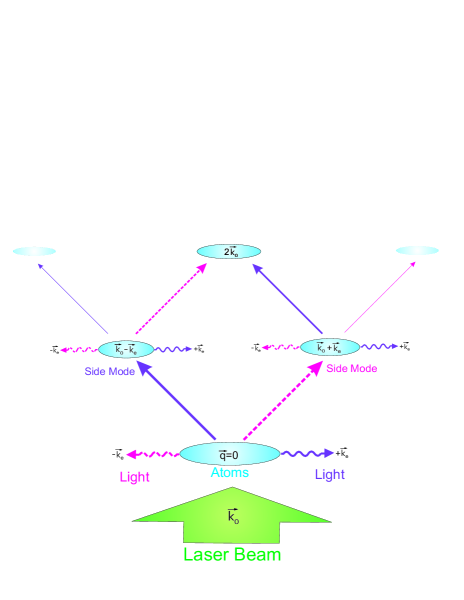
Figure 1: (Color online) A fan-like atomic side–mode pattern up to second order sequential superradiant scattering.

II.2 Effective Hamiltonian

The effective second quantized Hamiltonian, governing the dynamics of sequential SR system, is derived as follows. Due to the large energy scale difference between the center of mass (CM) dynamics for the atoms ($\sim$MHz) and the internal electronic degrees of freedom ($\sim$PHz), we can treat separately their respective motions. As in Ref. meystrePRA , the Hamiltonian of an atomic condensate with two level atoms interacting with a near-resonant laser pump, takes the following form

$$\hat{H} = \int d^{3}\mathbf{r}\hat{\psi}_{g}^{\dagger}(\mathbf{r})\left(-\frac{\hbar^{2}}{2m}\nabla^{2}+V_{\rm tg}(\mathbf{r})\right)\hat{\psi}_{g}(\mathbf{r})$$ (1)

$$+\int d^{3}\mathbf{r}\hat{\psi}_{e}^{\dagger}(\mathbf{r})\left(-\frac{\hbar^{2}}{2m}\nabla^{2}+V_{\rm te}(\mathbf{r})+\hbar\omega_{a}\right)\hat{\psi}_{e}(\mathbf{r})$$

$$+\int d^{3}\mathbf{k}\hbar\omega_{k}\hat{a}_{\mathbf{k}}^{\dagger}\hat{a}_{\mathbf{k}}$$

$$+\int d^{3}\mathbf{r}d^{3}\mathbf{k}\left[\hbar g^{*}(\mathbf{k})e^{-i\mathbf{k}\cdot\mathbf{r}}\hat{\psi}_{g}^{\dagger}(\mathbf{r})\hat{a}_{\mathbf{k}}^{\dagger}\hat{\psi}_{e}(\mathbf{r})\>+{\rm H.c.}\right],\hskip 12.0pt$$

under the dipole and rotating wave approximations. We have further neglected the static atom-atom interactions. The first two terms are the atomic Hamiltonians for the CM motion in their respective trapping potentials $(V_{\rm tg}(\mathbf{r})$, $V_{\rm te}(\mathbf{r}))$ of the internal states. The atomic fields, described by annihilation (creation) operator $\hat{\psi}_{g,e}(\mathbf{r})$ ($\hat{\psi}^{\dagger}_{g,e}(\mathbf{r})$), obey the usual bosonic algebra. $E_{g}=0$ and $E_{e}=\hbar\Delta=\hbar(\omega_{A}-\omega_{0})$ are the electronic excitation energies of the atom in the rotating frame defined by the pump laser field. The third term comes from the free electromagnetic field, while its interaction with the atoms is described with the last term ($\hat{H}_{af}$), which includes both the laser photons and the scattered photons. The operator $\hat{a}_{\mathbf{k}}$ ($\hat{a}^{\dagger}_{\mathbf{k}}$) annihilates (creates) a photon with wavevector $\mathbf{k}$, polarization $\hat{\epsilon}_{\mathbf{k}}$, and frequency $\omega_{\mathbf{k}}=ck-\omega_{0}$ (again in the rotating frame with frequency $\omega_{0}$). $g(\mathbf{k})=\left[c|\mathbf{k}|d^{2}/2\hbar\epsilon_{0}(2\pi)^{3}\right]^{1/2}|\hat{\mathbf{k}}\times\hat{\mathbf{x}}|$ is the dipole coupling coefficient, with $\vec{d}=\langle e|\vec{r}|g\rangle$ the matrix element for the atomic dipole transition.

In typical SR experiments ketterle , the detuning $\Delta\sim 10^{9}\,$Hz is much larger than both the CM motion energy scale $\sim 10^{6}\,$Hz or the Rabi frequency $\Omega_{0}\sim 10^{8}\,$Hz, the excited state operator can be eliminated adiabatically via replacing $\hat{\psi}_{e}(\mathbf{r})\approx-(1/\Delta)\left(\int d\mathbf{k}g(\mathbf{k})e^{i\mathbf{k}\cdot\mathbf{r}}\hat{a}_{\mathbf{k}}\right)\hat{\psi}_{g}(\mathbf{r})$ in the equations of motion, yielding an effective Hamiltonian

$$\hat{H} = \int d^{3}\mathbf{r}\hat{\psi}_{g}^{\dagger}(\mathbf{r})\left(-\frac{\hbar^{2}}{2m}\nabla^{2}+V_{\rm tg}(\mathbf{r})\right)\hat{\psi}_{g}(\mathbf{r})$$ (2)

$$+ \int d^{3}\mathbf{k}\hbar\omega_{k}\hat{a}_{\mathbf{k}}^{\dagger}\hat{a}_{\mathbf{k}}$$

$$- \frac{\hbar}{\Delta}\int d^{3}\mathbf{r}d^{3}\mathbf{k}d^{3}\mathbf{k}^{\prime}\tilde{g}(\mathbf{k},\mathbf{k}^{\prime},\mathbf{r})\hat{\psi}^{\dagger}_{g}(\mathbf{r})\hat{a}^{\dagger}_{\mathbf{k}}\hat{a}_{\mathbf{k}^{\prime}}\hat{\psi}_{g}(\mathbf{r}),$$

with $\tilde{g}(\mathbf{k},\mathbf{k}^{\prime},\mathbf{r})=g^{*}(\mathbf{k})g(\mathbf{k}^{\prime})\exp{({-i(\mathbf{k}-\mathbf{k}^{\prime})\cdot\mathbf{r}})}$, proportional to the effective coupling between the absorbed and subsequently emitted photons.

The atomic field operators can be expanded in terms of the quasi-particle excitations of BEC $\hat{\psi}_{g}(\mathbf{r})=\sum_{\mathbf{q}}\langle\mathbf{q}|\mathbf{r}\rangle\hat{c}_{\mathbf{q}}$, as described in Ref. meystre , with $\hat{c}_{\mathbf{q}}$ ($\hat{c}^{\dagger}_{\mathbf{q}}$) annihilating (creating) a scattered boson in the momentum side–mode $\mathbf{q}$ in the form $\langle\mathbf{r}|\mathbf{q}\rangle=\phi_{0}(\mathbf{r})e^{i\mathbf{q}\cdot\mathbf{r}}$. The initial condensate mode is described by the spatial wave function $\phi_{0}(\mathbf{r})$. The quasi modes for excitations approximately form an orthonormal basis because $\langle\mathbf{q}|\mathbf{q}^{\prime}\rangle=\delta_{\mathbf{q},\mathbf{q}^{\prime}}$. In the second quantized form within the side–mode representation Eq. (2) becomes

$$\hat{H} =\sum_{\mathbf{q}}\hbar\omega_{q}\hat{c}_{\mathbf{q}}^{\dagger}\hat{c}_{\mathbf{q}}+\int d^{3}\mathbf{k}\hbar\omega_{k}\hat{a}_{\mathbf{k}}^{\dagger}\hat{a}_{\mathbf{k}}$$ (3)

$$-\frac{\hbar}{\Delta}\sum_{\mathbf{q},\mathbf{q}^{\prime}}\int d^{3}\mathbf{k}d^{3}\mathbf{k}^{\prime}g^{*}(\mathbf{k})g(\mathbf{k}^{\prime})\rho_{\mathbf{q},\mathbf{q}^{\prime}}(\mathbf{k},\mathbf{k}^{\prime})\times$$

$$\times\hat{c}_{\mathbf{q}}^{\dagger}\hat{a}_{\mathbf{k}}^{\dagger}\hat{a}_{\mathbf{k}^{\prime}}\hat{c}_{\mathbf{q}^{\prime}},$$

where $\rho_{\mathbf{q},\mathbf{q}^{\prime}}(\mathbf{k},\mathbf{k}^{\prime})=\int d\mathbf{r}|\phi_{0}(\mathbf{r})|^{2}e^{i[(\mathbf{k}+\mathbf{q})-(\mathbf{k}^{\prime}+\mathbf{q}^{\prime})]\cdot\mathbf{r}}$ is the structure form factor of the condensate density, which is responsible for the highly directional emission of the end-fire mode photons. $\omega_{\mathbf{q}}=\hbar|\mathbf{q}|^{2}/2m$ is the side–mode energy at the recoil momentum of $\mathbf{q}$. The first two terms in Eq. (3) are diagonal in their respective Fock spaces and can be omitted by performing further rotating frame transformations $\hat{c}_{\mathbf{q}}\rightarrow\hat{c}_{\mathbf{q}}e^{-i\omega_{\mathbf{q}}t}$ and $\hat{a}_{\mathbf{k}}\rightarrow\hat{a}_{\mathbf{k}}e^{-i\omega_{\mathbf{k}}t}$. Thus, the effective Hamiltonian takes the form

$$\hat{H}=-\frac{\hbar}{\Delta}\sum_{\mathbf{q},\mathbf{q}^{\prime}}\int d^{3}\mathbf{k}d^{3}\mathbf{k}^{\prime}g^{*}(\mathbf{k})g(\mathbf{k}^{\prime})\rho_{\mathbf{q},\mathbf{q}^{\prime}}(\mathbf{k},\mathbf{k}^{\prime})\times$$

$$\times\hat{c}_{\mathbf{q}}^{\dagger}\hat{a}_{\mathbf{k}}^{\dagger}\hat{a}_{\mathbf{k}^{\prime}}\hat{c}_{\mathbf{q}^{\prime}}e^{i\left(\omega_{\mathbf{k}}+\omega_{q}-\omega_{\mathbf{k}^{\prime}}-\omega_{q^{\prime}}\right)t}.$$ (4)

In a sufficiently elongated condensate, large off-axis Rayleigh scattering is suppressed with respect to the end-fire modes mustecap . The angular distribution of the scattered light is sharply peaked at the axial directions ($\mathbf{k}_{e}=\pm k_{e}\hat{z}$), if the Fresnel number is larger than one ${\cal F}=W^{2}/L\lambda_{0}\gtrsim 1$ at the pump wavelength $\lambda_{0}$ for a condensate of length $L$ and width $W$ meystre . This makes it possible to consider only the axial end-fire modes. To investigate sequential SR, we further take into account the first order side–modes at $\mathbf{q}=\mathbf{k}_{0}\pm\mathbf{k}_{e}$ and the second order side–mode at $\mathbf{q}\approx 2\mathbf{k}_{0}$. The rest of the side–modes are assumed to remain unpopulated zobay . The Hamiltonian (4) that originally contains the contributions from all the side–modes and the end-fire modes as well as the laser field then reduces to the following simple model

$$\hat{H} = -\hbar\frac{g^{2}}{\Delta}\left(\hat{c}_{+}^{\dagger}\hat{a}_{-}^{\dagger}\hat{a}_{0}\hat{c}_{0}+\hat{c}_{-}^{\dagger}\hat{a}_{+}^{\dagger}\hat{a}_{0}\hat{c}_{0}\right.$$ (5)

$$\hskip 30.0pt\left.+\hat{c}_{2}^{\dagger}\hat{a}_{-}^{\dagger}\hat{a}_{0}\hat{c}_{-}+\hat{c}_{2}^{\dagger}\hat{a}_{+}^{\dagger}\hat{a}_{0}\hat{c}_{+}\right)+{\mathrm{H}.c.},$$

with $g\equiv g(\mathbf{k_{e}})$. We have adopted a shorthand notation where $\hat{a}_{\pm}\equiv\hat{a}_{\pm\mathbf{k}_{e}}$, $\hat{a}_{0}\equiv\hat{a}_{\mathbf{k}_{0}}$, $\hat{c}_{\pm}\equiv\hat{c}_{(\mathbf{k}_{0}\pm\mathbf{k}_{e})}$, and $\hat{c}_{2}\equiv\hat{c}_{2\mathbf{k}_{0}}$. This is the model Hamiltonian involving the interplay of the four atomic side–modes with three photonic modes. Before we further discuss and reveal the built-in entanglement swap mechanism for EPR-type quantum correlations in this model Hamiltonian, in the next section we shall briefly review continuous variable entanglement and extend its criteria to our case.

III Criteria for Continuous Variable Entanglement

The existence of continuous variable entanglement is determined by a sufficient condition on the inseparability of continuous variable states as given in Ref. duan2000 . If the density matrix of a quantum system is inseparable within two well defined modes duan2000 ; ping , or the two modes are entangled, the total variance of EPR-like operators, $\hat{u}=|c|\hat{x}_{1}+\hat{x}_{2}/c$ and $\hat{v}=|c|\hat{p}_{1}-\hat{p}_{2}/c$, satisfies the inequality

$$\langle\Delta\hat{u}^{2}\rangle+\langle\Delta\hat{v}^{2}\rangle<\left(c^{2}+1/c^{2}\right),$$ (6)

for a real number $c$, where $\hat{x}_{1,2}=(\hat{a}_{1,2}+\hat{a}_{1,2}^{\dagger})/\sqrt{2}$ and $\hat{p}_{1,2}=(\hat{a}_{1,2}-\hat{a}_{1,2}^{\dagger})/i\sqrt{2}$ are analogous to position and momentum operators as in the case of a simple harmonic oscillator. The indices corresponds to mode numbers.

Defining the inseparability parameter

$$\lambda=\langle\Delta\hat{u}^{2}\rangle+\langle\Delta\hat{v}^{2}\rangle-\left(c^{2}+1/c^{2}\right),$$ (7)

the presence of continuous variable entanglement is then characterized by the sufficient condition $\lambda<0$. For the two modes to be entangled, it suffices to find only one value of $c$ that leads to $\lambda<0$, and hence $c$ can be taken at which $\lambda$ is minimum.

The parameter $\lambda$ we adopt here clearly corresponds to an entanglement witness, but not an entanglement measure. Because the states for more negative $\lambda$ do not necessarily correspond to more entangled states.

The total variance of the EPR operators are bounded below by the Heisenberg uncertainty relation $\langle\Delta\hat{u}^{2}\rangle+\langle\Delta\hat{v}^{2}\rangle\geq\left|c^{2}-1/c^{2}\right|$. Thus, $\lambda$ has a lower bound $\lambda_{\text{low}}=\left|c^{2}-1/c^{2}\right|-\left(c^{2}+1/c^{2}\right)$.

After minimization with respect to $c$, a more explicit expression of $\lambda$ can be given as

$$\lambda= 2\left(c^{2}\langle\hat{a}^{\dagger}_{1}\hat{a}_{1}\rangle+\langle\hat{a}^{\dagger}_{2}\hat{a}_{2}\rangle/{c^{2}}+\text{sign}(c)\langle\hat{a}_{1}\hat{a}_{2}+\hat{a}^{\dagger}_{1}\hat{a}^{\dagger}_{2}\rangle\right)$$ (8)

$$-\langle\hat{u}\rangle^{2}-\langle\hat{v}\rangle^{2},$$

where $c^{2}=\left[(\langle\hat{a}^{\dagger}_{-}\hat{a}_{-}\rangle-|\langle\hat{a}_{-}\rangle|^{2})/(\langle\hat{a}^{\dagger}_{+}\hat{a}_{+}\rangle-|\langle\hat{a}_{+}\rangle|^{2})\right]^{1/2}$ with $\text{sign}(c)=-\text{sign}\left[\text{Re}\left\{\langle\hat{a}_{+}\hat{a}_{-}\rangle\right\}-\alpha_{+}\alpha_{-}+\beta_{+}\beta_{-}\right]$, $\alpha_{\pm}=\text{Re}\left\{\langle\hat{a}_{\pm}\rangle\right\}$ and $\beta_{\pm}=\text{Im}\left\{\langle\hat{a}_{\pm}\rangle\right\}$.

In the system we study here, the bosonic mode operators will be either end-fire mode pairs $a_{1,2}=a_{\pm}$ or end-fire modes and first side–modes, $a_{1}=a_{\pm},a_{2}=c_{\mp}$. Unlike other model investigations ping of EPR-like correlations based upon $\lambda$, we need to keep track of the $\langle\hat{u}\rangle^{2}$ and $\langle\hat{v}\rangle^{2}$ terms, because $\langle\hat{x}_{1,2}\rangle$ and $\langle\hat{p}_{1,2}\rangle$ do not necessarily vanish for our model during time evolution. Furthermore, since the time evolution of the two end-fire modes are symmetric in our case, we find $c^{2}=1$ and $\lambda_{\text{low}}=-2$.

In the remainder of this paper, we examine the time evolution of the continuous variable entanglement witness $\lambda(t)$ both for the opposite end-fire modes and for the end-fire modes with side–modes. This study is expected to provide insight into the temporal development and the swap of quantum correlations between different sub-systems/modes. The following section is aimed at establishing an intuitive understanding of how EPR-like correlations between opposite end-fire modes are built up.

IV An entanglement Swap Mechanism

In sec. VI we will exhibit the numerical results for the time evolution of the entanglement parameter $\lambda(t)$, governed by the Hamiltonian (5). We will observe that, there exists regions in time where $\lambda$ becomes negative, i.e., conclusive evidence for the presence of entanglement during dynamical evolution. In this section, we hope to provide an intuitive understanding to support the result revealed through the numerical approach. We will show that it is due to the presence of an inherent swap mechanism which leads to the generation of the EPR photon pair. We shall examine the dynamical behavior of the system in two different time regimes, the early times when the first side–modes just start to grow and the later times when the second order side–mode contributes to the dynamics.

IV.1 Early Times

In the initial stage, occupation of the second order side–mode ($|c_{2}\rangle$) can be neglected. During this initiation period of the short-time dynamics, the number of atoms in the zero-momentum state can be assumed undepleted $\hat{c}_{0}\approx\sqrt{N}e^{i\phi_{1}}$ with a constant $N$ standing for the number of condensed atoms, like in the treatment of degenerate parametric processes. Since the pump is very strong, and the number of pump photons are much larger than the number of condensate atoms $M\gg N$, it can also be treated within the parametric pump approximation $\hat{a}_{0}\approx\sqrt{M}e^{i\theta_{0}}$ as undepleted. Thus, the initial behavior of the system is governed by the Hamiltonian

$$\hat{H}_{1}=-\hbar\chi_{1}\left[e^{i\theta_{1}}\left(\hat{a}_{+}^{\dagger}\hat{c}_{-}^{\dagger}+\hat{a}_{-}^{\dagger}\hat{c}_{+}^{\dagger}\right)+{\rm H.c.}\right],$$ (9)

with $\chi_{1}=\sqrt{NM}|g|^{2}/\Delta$ and $\theta_{1}=\theta_{0}+\phi_{1}$ is the initial phases difference. This form of $\hat{H}_{1}$ is exactly the same as that of two uncoupled optical parametric amplifiers (OPAs). It allows for the growth of the first-order side–modes meystre as well as the entanglement of side–mode atoms with the end-fire mode photons paris . The solution to $\hat{H}_{1}$ in the Heisenberg picture is given by the following time dependencies of operators mandel

$$\hat{a}_{\pm}(t)=\text{cosh}(\chi_{1}t)\hat{a}_{\pm}+ie^{i\theta}\text{sinh}(\chi_{1}t)\hat{c}_{\mp}^{\dagger},$$ (10)

$$\hat{c}_{\pm}(t)=\text{cosh}(\chi_{1}t)\hat{c}_{\pm}+ie^{i\theta}\text{sinh}(\chi_{1}t)\hat{a}_{\mp}^{\dagger},$$ (11)

where the operators without time arguments are at the initial time.

The side–modes and the end-fire modes are initially unoccupied $|a_{+},a_{-},c_{+},c_{-}\rangle=|0,0,0,0\rangle$, or taken to be in their respective vacuum states. The time dependencies for the populations of the side–modes and end-fire modes come out as $\langle\hat{I}_{\pm}\rangle=\langle\hat{n}_{\pm}\rangle=\text{sinh}^{2}(\chi_{1}t)$, analogous to the classical results mandel . Evaluating correlations between the two end-fire modes (e), we find

$$\lambda\equiv\lambda_{\text{ee}}=4\text{sinh}^{2}(\chi_{1}t),$$ (12)

which is always positive $\lambda_{\text{ee}}>0$. On the other hand, the correlation between the end-fire mode (e) and side–mode (s), scattered in the opposite directions, takes the following form

$$\lambda_{\text{se}}=2\left[2\text{sinh}^{2}(\chi_{1}t)-|\text{sin}(\theta_{1})|\text{sinh}(2\chi_{1}t)\right],$$ (13)

which starts with $\lambda_{\text{se}}(t)=0$ and evolves down to $\lambda_{\text{se}}(t_{0}\gtrsim 2)\simeq-2$, the lowest possible value of $\lambda_{\text{low}}=-2$ imposed by the Heisenberg uncertainty, at $|\sin(\theta_{1})|\simeq 1$.

In Figs. 3(a) and 3(b), this is further supported by more elaborate results from numerical calculations of $\lambda$ and $\lambda_{\text{se}}$. Same conclusions can be seen for the analytical results (12) over the range $t=0$-$t=0.3$ms in Fig. 3(a) and (13) over the range $t=0$-$0.2$ms in Fig. 3(b).

IV.2 Later Times

At later times, the first-order side–modes become effectively populated, giving rise to noticeable second sequence of SR from the edges of these side–mode condensates. In this case, the occupancy for the $|c_{0}\rangle$ mode is not an important issue, but the $|c_{2}\rangle$ mode becomes populated due to the second order SR.

We construct an approximate model by assuming that the occupation of $|c_{2}\rangle$ is not changing too much, or effective treating it as in in the steady state with $\hat{c}_{2}\approx\sqrt{N_{2}}e^{-i\phi_{2}}$. $N_{2}$ is the number of atoms in the $|c_{2}\rangle$ state. The later stage dynamics of the system, where the $\text{2}^{\text{nd}}$ order SR is effective, is then governed by the model Hamiltonian

$$\hat{H}_{2}=-\hbar\chi_{2}\left[e^{i\theta_{2}}\left(\hat{a}_{-}^{\dagger}\hat{c}_{-}+\hat{a}_{+}^{\dagger}\hat{c}_{+}\right)+{\rm H.c.}\right],$$ (14)

with $\chi_{2}=\sqrt{N_{2}M}|g|^{2}/\Delta$ and $\theta_{2}=\bar{\theta}_{0}+\phi_{2}$. As before we again neglect the depletion of the pump $\hat{a}_{0}\approx\sqrt{M}e^{i\bar{\theta}_{0}}$.

This model $\hat{H}_{2}$ is also exactly solvable. The time dependencies of the annihilation operators in the Heisenberg picture are

$$\hat{a}_{\pm}(t) = \text{cos}(\chi_{2}\Delta t)\hat{a}_{\pm}+ie^{i\phi_{2}}\text{sin}(\chi_{2}\Delta t)\hat{c}_{\pm},$$ (15)

$$\hat{c}_{\pm}(t) = \text{cos}(\chi_{2}\Delta t)\hat{c}_{\pm}+ie^{-i\phi_{2}}\text{sin}(\chi_{2}\Delta t)\hat{a}_{\pm},$$ (16)

where $t>t_{0}$, the operators without time arguments are at $t=t_{0}$, and $\Delta t=t-t_{0}$. We can approximately connect these two models together into smooth temporal dynamics if we use the solutions of $\hat{H}_{1}$ as the initial state for dynamics due to $\hat{H}_{2}$ so that $\hat{a}_{\pm}(t_{0})$ and $\hat{c}_{\pm}(t_{0})$ are calculated at $t=t_{0}$ from the equations (10) and (11), respectively. We define $t_{0}$ as the time at which all the $|c_{0}\rangle$ atoms are scattered into the side–modes, and thus it is determined from $\text{sinh}^{2}(\chi_{1}t_{0})=N/2$.

In this later dynamical stage, the entanglement witness parameter in between the end-fire modes (e) is evaluated to be ($\lambda\equiv\lambda_{\text{ee}}$)

$$\lambda(t) = 4\text{sinh}^{2}(\chi_{1}t_{0})$$ (17)

$$- |\text{cos}(\bar{\theta})\text{sin}(2\chi_{2}\Delta t)|\text{sinh}(2\chi_{1}t_{0}),$$

where $\bar{\theta}=\theta_{1}+\theta_{2}$. When $|\cos(\bar{\theta})|\simeq 1$, $\lambda$ evolves from $2N$ down to the minimum possible negative value of $\lambda_{\text{low}}=-2$, at $\Delta t=\pi/4\chi_{2}$. An analogous calculation for entanglement between the end-fire mode (e) and side–mode (s) gives

$$\lambda_{\text{se}}(t) = 4\text{sinh}^{2}(\chi_{1}t_{0})$$ (18)

$$- 2|\text{sin}(\theta_{2})\text{cos}(2\chi_{2}\Delta t)|\text{sinh}(2\chi_{1}t_{0}),$$

which starts at $\lambda_{\text{se}}(t_{0})=-2$ and increases to values of order $\sim N$, for proper choices of $\theta_{2}$. Many of these features revealed from simple analytic models find their parallels in numerical solutions as displayed in Fig. 3.

The results from the two model Hamiltonians are found to depend on the initial phase difference between $\theta_{1}$ and $\theta_{2}$, but not the individual phases. Such a phase dependence of the results is analogous to the cases of parametric down conversion and the two-mode squeezing mandel . The phases introduced in the second stage reflects the accumulating temporal phase difference of the operators through the time evolution. In the numerical calculation it is sufficient to assign initial phases for the pump laser and the condensate or just their difference.

Without any detailed analysis, simply consider the behaviors of Eqs. (13) and (17) instead, one can already appreciate the built-in entanglement swap mechanism within the superradiant BEC in action. The entanglement created between the side–mode and end-fire mode Eq. (13) in the initial stage, is swapped to entanglement between the two end-fire modes Eq. (17), due to the $\text{2}^{\text{nd}}$ order SR. The model Hamiltonian $\hat{H}_{1}$ couples the $|a_{\pm}\rangle\leftrightarrow|c_{\mp}\rangle$ modes, but leaves $|a_{+}\rangle\leftrightarrow|a_{-}\rangle$ modes decoupled at the initial times. The model Hamiltonian $\hat{H}_{2}$, at later times, couples the $|a_{\pm}\rangle\leftrightarrow|c_{\pm}\rangle$ states. Two noninteracting modes $|a_{+}\rangle\leftrightarrow|a_{-}\rangle$ are coupled through their common interaction with the same side–mode, and become entangled due to the swap mechanism.

V Numerical Calculation of the Entanglement Parameter

We study the dynamics of the entanglement parameter $\lambda(t)$ and the accompanying populations for the fields ($I_{0}(t)$,$I_{\pm}(t)$) and the atomic states ($n_{0}$,$n_{\pm}(t)$,$n_{2}$). Their complete temporal evolution is governed by the Hamiltonian Eq. (5). Our calculation will be numerically obtained, aided by a decorrelation approximation that neglects higher order correlations. The numerical results will be illustrated and discussed in the next section.

The entanglement parameter $\lambda$, given in Eq. (8), is determined by the expectation values of both $\hat{a}_{\pm}$ operators and their products. Their equations of motion in operator forms can be derived from the full Hamiltonian Eq. (5). The dynamics of two operator products is found to depend on four operator products; and four operator products depend on six operator products, and so on so forth. Such a hierarchy of operator equations is impossible to manage in general.We therefore resort to a decorrelation approximation that truncates it to a closed form. The usual treatment of this kind andreev for the SR system closes the chain early by a simple decorrelation of atomic and optical operators, which is clearly inappropriate when entanglement swap is to be studied.

We adopt a decorrelation rule that factorizes condensate and the second order side–mode operators in operator products. Since quantum correlations between the condensate and other modes are expected to be weak due to the almost classical, coherent-state-like nature for the condensate and its diminishing population when the second order side–mode is significantly populated at later stages of dynamics. Operators for the pump photons will also be factorized, again relying on the almost classical, coherent state nature of the pump field.

Our approach makes it possible to keep quantum correlations between the end-fire modes and the intermediate side–modes. The hierarchy of equations is closed under $\langle xyz\rangle\approx\langle xy\rangle\langle z\rangle$, with $x,y\in\{1,c_{\pm},c_{\pm}^{\dagger},a_{\pm},a_{\pm}^{\dagger}\}$ and $z\in\{c_{0},c_{0}^{\dagger},c_{2},c_{2}^{\dagger}\}$. The resulting equations, governing the dynamics of the expectations, are given in the Appendix. These equations are solved numerically.

For the initial conditions, both the end-fire modes and side–modes are taken to be their vacuum Fock states while the laser and the condensate are in coherent states. We consider a system with typical parameters of a condensate with number of atoms $N=8\times 10^{6}$ and a pump with $M=2\times 10^{8}$ photons. Additionally, phenomenological decoherence rates are introduced by assuming the same damping rates mustecap for the atomic and photonic modes. The decay rates are obtained from the effective decay of the experimentally measured contrast for the atomic density distribution pattern ketterle . In addition, we also explored an interesting scheme where the coupled equations (19-36) were solved, in the presence of phenomenological damping, for an initial two-mode squeezed vacuum (for the end-fire modes) with a squeezing parameter $\xi=r\exp{(i\theta_{r})}$.

VI Results and Discussion

In sec. IV we discussed the origins of the entanglement swap in sequential SR. In this section, in order to provide for a more detailed and quantitative understanding, we present results obtained from numerical calculations. We will discuss the time evolution of the entanglement parameter $\lambda(t)$, between the two end-fire modes, within the parameter regime of the experiment ketterle . At first, we will disregard decoherence and examine the nature of fully coherent sequential dynamics. We will show that $\lambda$ attains negative values, confirming the presence of entanglement due to the swap mechanism as we intuitively discussed in the previous section. We then introduce effective damping rates specific to the experimental situation. Finally, we will examine the effect of initializing the quantum dynamics of our model system from in a two-mode (end-fire modes) squeezed vacuum, in the presence of decoherence and dissipations. We will end with investigations of the dependence of correlations on the number of condensate atoms.

VI.1 Dynamics of Entanglement

In Fig. 2, we plot the temporal evolution of optical field intensities and atomic side–mode populations. The plot is found to be totally symmetric with respect to $t=t_{c}=0.35$ ms. The peak in the intensity after $t_{c}$ is the analog of the Chiao ringing chiao . In the experiments such a complete ringing cannot be observed due to the presence of decoherence, which will be taken into account in our subsequent calculations.

In Fig. 3, we plot the temporal evolution of entanglement parameters $\lambda_{\text{ee}}$ (photon-photon) and $\lambda_{\text{se}}$ (atom-photon) over the population dynamics, depicted in Fig. 2. The lower panel of Fig. 3 demonstrates the swap dynamics. The initial atom-photon entanglement ($\lambda_{\text{se}}$) is seen to evolve continuously into entanglement between the two end-fire modes ($\lambda$). Both the parameters $\lambda_{\text{se}}$ and $\lambda$ is found to be able to reach down to the lowest possible value, $\lambda_{\text{low}}=-2$, set by the Heisenberg uncertainty principle (as in sec. III). The complete numerical results match well with the analytic solutions, discussed previously in Sec. IV, for the model Hamiltonians (9) at early times and (14) at later times.

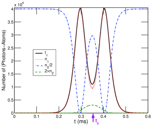
Figure 2: (Color online) The temporal evolutions for atomic side–mode populations and optical field intensities. $I_{\pm}$, $n_{\pm}$, $n_{0}$, and $n_{2}$ denote occupancy numbers of bosonic modes $|a_{\pm}\rangle$, $|c_{\pm}\rangle$, $|c_{0}\rangle$, and $|c_{2}\rangle$, respectively. $n_{\pm}(t)$ and $I_{\pm}(t)$ overlap except for a short time interval near $t=t_{c}=0.35$ms. Notice that $n_{0}$ and $n_{2}$ are scaled for visual clarity.

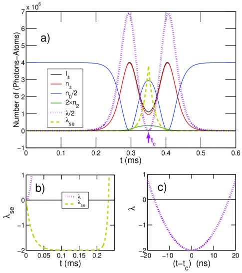
Figure 3: (Color online) (a) The temporal evolutions of atom-photon ($|a_{\pm}\rangle\leftrightarrow|c_{\mp}\rangle$) and photon-photon ($|a_{+}\rangle\leftrightarrow|a_{-}\rangle$) mode correlations as evidenced by the entanglement parameters $\lambda_{\text{se}}$ and $\lambda\equiv\lambda_{\text{ee}}$, respectively. Accompanying population dynamics (Fig. 2) is also plotted in the background. (b) an expanded view of the early time dynamics for $\lambda_{\text{se}}$ and $\lambda$; (c) an expanded view of $\lambda$ around $t_{c}=0.35$ ms.

In the time interval of $t=0$-$0.30$ ms, we find the system is dominated by the $1^{\text{st}}$ sequence of SR. The atomic condensate, initially in the zero-momentum state $|c_{0}\rangle$, is pumped into the $1^{\text{st}}$ order side–modes $|c_{\pm}\rangle$. This is the reason for the overlap of $n_{\pm}(t)$ with $I_{\pm}(t)$ during this interval. Due to the interaction between the side–modes and the end-fire modes, scattered into opposite directions, $\lambda_{\text{se}}$ becomes negative in this region.

When the $|c_{\pm}\rangle$ side–modes become maximally occupied at about $t=0.30\,$ms, the $1^{\text{st}}$ sequence of SR is completed. At this time, these side–modes are sufficiently populated to give rise to the $2^{\text{nd}}$ sequence of SR. In the interval $t=0.30$-$0.35\,$ms atoms in the side–modes $|c_{\pm}\rangle$ are pumped into the $2^{\text{nd}}$ order side–mode $|c_{2}\rangle$. The majority of the populations, however, oscillates back to the $|c_{0}\rangle$ mode because of the more dominant Rabi oscillation between the $|c_{0}\rangle$ and $|c_{\pm}\rangle$ modes. Two other reasons also contribute to the repopulation of the condensate mode: first, the neglect of the propagational induced departure of the end-fire mode photons from the atomic medium; and second, the neglect of the other two $2^{\text{nd}}$ order side–modes $|c_{2\mathbf{k_{0}}\pm 2\mathbf{k_{e}}}\rangle$ for atoms to get into. Two end-fire modes get indirectly coupled by the entanglement swapping and between $t=0.30$-$0.35$ ms $\lambda(t)$ gradually becomes negative.

Entanglement of the end-fire modes arises at $t=t_{c}=0.35$ ms, when the $|c_{2}\rangle$ mode is maximally occupied as shown in Fig. 3. The minimum value of $\lambda$, which occurs at $t=t_{c}$, is found to coincide with the maximum value of $n_{2}(t)$.

When $t>t_{c}$, however, due to our limited mode approximation of not including even higher side–modes, we cannot study any effects which could potential give rise to higher order correlations, such as the onset of the $3^{\text{rd}}$ sequence of SR. The oscillatory Chiao type ringing revivals in the present result after $t>t_{c}$ mainly arise from the exclusion of decoherence, dephasing, dissipations, and the higher order side–modes in the model system. In the present work, we limited ourselves to a particular side–mode pattern as actually observed in available experiments ketterle . Despite its simplicity, we find our model can reasonably explain effects of decoherence and dephasing on the entanglement dynamics, which is further illustrated in the next subsection.

VI.2 Vacuum squeezing and Decoherence

The introduction of experimentally reported decoherence rate of $\gamma/2\pi=1.3\times 10^{4}$ Hz phenologically into the dynamical equations for the coupled system is found to not change the nature of the entanglement and swap dynamics significantly, which is supported by the numerical results shown in Fig. 4. We find that $\lambda$ can still become negative in certain time window, although it now stops short of reaching the theoretical lower bound of $-2$.

In the lower panel in Fig. 4 the temporal window for the negative values of $\lambda$, or the presence of entanglement is found to become narrower and the minimum value of $\lambda$, $\lambda_{\text{min}}$, is now somewhat larger for stronger decoherence, as may be expected. According to sec. III, a less negative value of $\lambda$ does not necessarily imply less entanglement, because $\lambda$ is simply an entanglement witness parameter but not an entanglement measure. On the other hand, it is still beneficial to aim for lower values of $\lambda$, because the numerical results we obtain associate lower values with longer entanglement durations, and furthermore more tolerant to decoherence, which means photon-photon entanglement can withstand the higher decoherence rates.

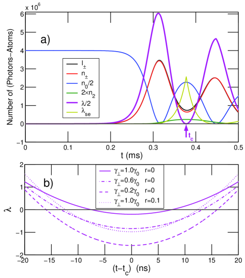
Figure 4: (Color online) (a) The temporal evolution of atomic and field mode populations, and of entanglement parameters. A decoherence rate of $\gamma_{0}/2\pi=1.3\times 10^{4}$Hz is introduced without any initial squeezing. (b) An expanded view of the dependence of $\lambda$ on decoherence rate $\gamma$ and squeezing parameter $r$ around $t_{c}=0.38$ ms.

For this aim, we choose to consider end-fire modes which are initially in two-mode squeezed vacuum states. The lower panel in Fig. 4 shows that an initially two-mode squeezed vacuum, for the end-fire modes, can indeed compensate to a certain degree for decoherence. This shows that, initially induced two-mode squeezing (or entanglement) in between the end-fire modes enhances their subsequent entanglement after the entanglement swap.

This observation can be interpreted as follows based on the numerical results. Any initial correlation between the end-fire modes is lost in the early dynamical stage where the end-fire modes are entangled with the first side–modes. The presence of initial correlation, however, causes the resultant atom-photon entanglement to be more resistant to decoherence. As a result, photon-photon correlations established by swapping from the atom-photon correlations in the subsequent dynamical stage also become more resistant to decoherence.

Finally, we examine the influence on $\lambda$ from the number of atoms in a condensate. We find that, as illustrated in Fig. 5, $\lambda_{\text{min}}$ becomes more negative for larger condensates. In the small condensate limit, $\lambda_{\text{min}}$ is found to decrease linearly with $N$ when the Fock vacuum is considered as initial conditions for other modes. The lower limit of $-2$ is never attained. When a small amount of initial squeezing is introduced, however, $\lambda$ can be brought down to theoretical minimum of $-2$. It approaches $-2$ in the large condensate limit with or without any help from initial squeezing in the two end-fire modes.

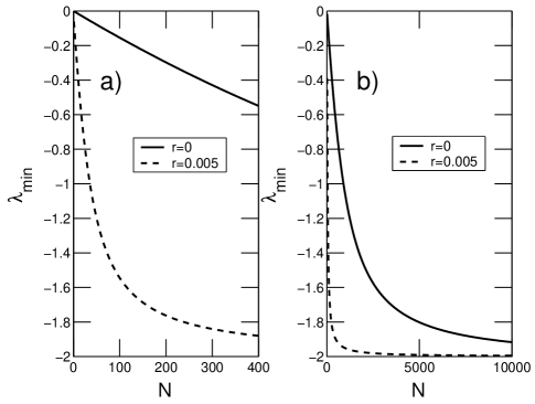
Figure 5: The dependence of $\lambda_{\rm min}$ on $N$ in different scales. Solid lines are for an initial coherent vacuum ($r=0$) and dashed lines are for a squeezed vacuum ($r=0.005$ and $\theta=\pi)$.

In addition to the amplitude of squeezing parameter, its phase could also influence $\lambda_{\rm min}$. In Fig. 6, we plot the minimum value of the entanglement parameter as a function of the phase and amplitude of the squeezing parameter $\xi=re^{i\theta_{r}}$. We performed this study for a small condensate with $N=100$ atoms and ignored the phenological decoherence. We find that the most efficient enhancement occurs along the line $\theta_{r}=\pi$. For larger condensates we find that the center of Fig. 6, where $\lambda>0$, spreads out to the $\theta_{r}=0$ and $\theta_{r}=\pi$ edges, as $N$ is increased. Entanglement is enhanced mainly along $\theta_{r}=0$ and $\theta_{r}=\pi$ lines.

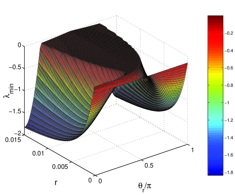
Figure 6: (Color online) The dependence of $\lambda_{\rm min}$ on $r$ and $\theta_{r}$ for $N=100$. $\lambda_{\rm min}$ shows a mirror symmetry for $\theta_{r}>\pi$.

VII Conclusions

We investigate photon-photon entanglement between the counter-propagating end-fire modes, of a sequentially superradiant atomic Bose-Einstein condensate. We calculate the temporal evolution of the continuous variable entanglement witness parameter for suitable realistic experimental parameters in the cw-pump laser regime ketterle , and find that EPR like correlations can be generated between the oppositely directed end-fire modes, despite the fact that they do not directly interact.

The generation of entanglement is shown to be due to a built-in entanglement swap mechanism we uncover in the sequential SR system. It is shown that end-fire mode photons become entangled immediately after the second sequence of the superradiance. In the second sequence, one of the end-fire modes interacts with the side–mode, with which the other end-fire mode has already interacted before in the first sequence. This mechanism allows for swapping the entanglement established between the end-fire modes and the side–modes in the first sequence, to the entanglement of the end-fire modes per se.

Increasing the number of atoms in the condensate, or initializing superradiance with a two-mode squeezed vacuum (for the end-fire modes), are found to be beneficial to the efficient construction of entanglement between end-fire modes, via the increasing of entanglement durations and making the entanglement more tolerant to decoherence.

The initial phase difference of the incoming pump laser and the condensate, the phase and the amplitude of the squeezing parameter for the end-fire mode vacuum, the number of atoms in a condensate and its geometric shape, all play certain roles in order to achieve the optimum ERP-like correlations in between the end-fire modes and these parameters are discussed in detail in the present manuscript for the cases of both small and large condensates.

Appendix A

We calculate temporal evolution of entanglement parameter $\lambda(t)$, given in (8), starting from the Heisenberg operator equations, obtained from (5). We evaluate the expectations for both single operators and two operator products. We arrive at a closed set from the expectations via performing decorrelation approximation, in parallel with the development and understanding of the swap mechanism (Sec. IV).

The resulting closed set of equations for expectation values are given through Eqs. (19-36), where time is scaled by frequency $\alpha=g^{2}/2\Delta$ with $g\simeq 2\times 10^{3}$ Hz, while operators are not scaled. $\alpha$ is related to $\gamma$ of Ref. mustecap , as $\gamma=\sqrt{M}\alpha=10.7$ Hz. Phenological decay rates can be introduced in Eqs. (19-36) by scaling $\gamma_{\perp}=1.3\times 10^{4}$Hz with $\alpha$. However, since the decay rates are introduced, in mustecap , for three-operator products, we use $\gamma_{\perp}/3$ for single operators and $2\gamma_{\perp}/3$ for two operator products. We have also checked the parallelism of our density dynamics with mustecap , which are in good agreement with the experiment ketterle .

$$\frac{d\langle a_{\pm}\rangle}{dt} = i\langle a_{0}\rangle\Big{(}\langle c_{\mp}^{\dagger}\rangle\langle c_{0}\rangle+\langle c_{2}^{\dagger}\rangle\langle c_{\pm}\rangle\Big{)},$$ (19)

$$\frac{d\langle a_{0}\rangle}{dt} = i\Big{(}\langle a_{-}c_{+}\rangle\langle c_{0}^{\dagger}\rangle+\langle a_{-}c_{-}^{\dagger}\rangle\langle c_{2}\rangle$$ (20)

$$+ \langle a_{+}c_{-}\rangle\langle c_{0}^{\dagger}\rangle+\langle a_{+}c_{+}^{\dagger}\rangle\langle c_{2}\rangle\Big{)},$$

$$\frac{d\langle c_{\pm}\rangle}{dt} = i\Big{(}\langle a_{0}\rangle\langle a_{\mp}^{\dagger}\rangle\langle c_{0}\rangle+\langle a_{0}\rangle^{*}\langle a_{\pm}\rangle\langle c_{2}\rangle\Big{)},$$ (21)

$$\frac{\langle c_{0}\rangle}{dt} = i\langle a_{0}\rangle^{*}\Big{(}\langle a_{-}c_{+}\rangle+\langle a_{+}c_{-}\rangle\Big{)},$$ (22)

$$\frac{\langle c_{2}\rangle}{dt} = i\langle a_{0}\rangle\Big{(}\langle a_{-}^{\dagger}c_{-}\rangle+\langle a_{+}^{\dagger}c_{+}\rangle\Big{)},$$ (23)

$$\frac{d\langle a_{+}a_{-}\rangle}{dt} = i\langle a_{0}\rangle\Big{(}\langle a_{-}c_{-}^{\dagger}\rangle\langle c_{0}\rangle+\langle a_{-}c_{+}\rangle\langle c_{2}^{\dagger}\rangle$$ (24)

$$+ \langle a_{+}c_{+}^{\dagger}\rangle\langle c_{0}\rangle+\langle a_{+}c_{-}\rangle\langle c_{2}^{\dagger}\rangle\Big{)},$$

$$\frac{d\langle a_{+}a_{-}^{\dagger}\rangle}{dt} = i\Big{(}\langle a_{0}\rangle\langle a_{-}^{\dagger}c_{-}^{\dagger}\rangle\langle c_{0}\rangle+\langle a_{0}\rangle\langle a_{-}^{\dagger}c_{+}\rangle\langle c_{2}^{\dagger}\rangle$$ (25)

$$- \langle a_{0}\rangle^{*}\langle a_{+}c_{+}\rangle\langle c_{0}^{\dagger}\rangle+\langle a_{0}\rangle^{*}\langle a_{+}c_{-}^{\dagger}\rangle\langle c_{2}\rangle\Big{)},$$

$$\frac{d\langle a_{\pm}^{2}\rangle}{dt} = 2i\langle a_{0}\rangle\Big{(}\langle a_{\pm}c_{\mp}^{\dagger}\rangle\langle c_{0}\rangle+\langle a_{\pm}c_{\pm}\rangle\langle c_{2}^{\dagger}\rangle\Big{)},$$ (26)

$$\frac{d\langle c_{+}c_{-}\rangle}{dt} = i\Big{(}\langle a_{0}\rangle\langle a_{-}^{\dagger}c_{-}\rangle\langle c_{0}\rangle+\langle a_{0}\rangle^{*}\langle a_{+}c_{-}\rangle\langle c_{2}\rangle$$ (27)

$$+ \langle a_{0}\rangle\langle a_{+}^{\dagger}c_{+}\rangle\langle c_{0}\rangle+\langle a_{0}\rangle^{*}\langle a_{-}c_{+}\rangle\langle c_{2}\rangle\Big{)},$$

$$\frac{d\langle c_{+}c_{-}^{\dagger}\rangle}{dt} = i\Big{(}\langle a_{0}\rangle\langle a_{-}^{\dagger}c_{-}^{\dagger}\rangle\langle c_{0}\rangle+\langle a_{0}\rangle^{*}\langle a_{+}c_{-}^{\dagger}\rangle\langle c_{2}\rangle$$ (28)

$$- \langle a_{0}\rangle^{*}\langle a_{+}c_{+}\rangle\langle c_{0}^{\dagger}\rangle-\langle a_{0}\rangle\langle a_{-}^{\dagger}c_{+}\rangle\langle c_{2}^{\dagger}\rangle\Big{)},$$

$$\frac{\langle c_{\pm}^{2}\rangle}{dt} = 2i\Big{(}\langle a_{0}\rangle\langle a_{\mp}^{\dagger}c_{\pm}\rangle\langle c_{0}\rangle$$ (29)

$$+ \langle a_{0}\rangle^{*}\langle a_{\pm}c_{\pm}\rangle\langle c_{2}\rangle\Big{)},$$

$$\frac{d\langle a_{\pm}c_{\mp}\rangle}{dt} = i\Big{(}\langle a_{0}\rangle\langle c_{\mp}^{\dagger}c_{\mp}\rangle\langle c_{0}\rangle+\langle a_{0}\rangle\langle c_{\pm}c_{\mp}\rangle\langle c_{2}^{\dagger}\rangle$$ (30)

$$+ \langle a_{0}\rangle\langle a_{\pm}a_{\pm}^{\dagger}\rangle\langle c_{0}\rangle+\langle a_{0}\rangle^{*}\langle a_{\pm}a_{\mp}\rangle\langle c_{2}\rangle\Big{)},$$

$$\frac{d\langle a_{\pm}c_{\pm}^{\dagger}\rangle}{dt} = i\Big{(}\langle a_{0}\rangle\langle c_{\pm}^{\dagger}c_{\mp}^{\dagger}\rangle\langle c_{0}\rangle+\langle a_{0}\rangle\langle c_{\pm}c_{\pm}^{\dagger}\rangle\langle c_{2}^{\dagger}\rangle$$ (31)

$$- \langle a_{0}\rangle^{*}\langle a_{\pm}a_{\mp}\rangle\langle c_{0}^{\dagger}\rangle-\langle a_{0}\rangle^{*}\langle a_{\pm}a_{\pm}^{\dagger}\rangle\langle c_{2}^{\dagger}\rangle\Big{)},$$

$$\frac{\langle a_{\pm}c_{\pm}\rangle}{dt} = i\Big{(}\langle a_{0}\rangle\langle c_{\pm}c_{\mp}^{\dagger}\rangle\langle c_{0}\rangle+\langle a_{0}\rangle\langle c_{\pm}^{2}\rangle\langle c_{2}^{\dagger}\rangle$$ (32)

$$+ \langle a_{0}\rangle\langle a_{\pm}a_{\mp}^{\dagger}\rangle\langle c_{0}\rangle+\langle a_{0}\rangle^{*}\langle a_{\pm}^{2}\rangle\langle c_{2}\rangle\Big{)},$$

$$\frac{\langle c_{\pm}^{\dagger}c_{\pm}\rangle}{dt} = i\Big{(}-\langle a_{0}\rangle^{*}\langle a_{\mp}c_{\pm}\rangle\langle c_{0}^{\dagger}\rangle-\langle a_{0}\rangle\langle a_{\pm}^{\dagger}c_{\pm}\rangle\langle c_{2}^{\dagger}\rangle$$ (33)

$$+ \langle a_{0}\rangle\langle a_{\mp}^{\dagger}c_{\pm}^{\dagger}\rangle\langle c_{0}\rangle+\langle a_{0}\rangle^{*}\langle a_{\pm}c_{\pm}^{\dagger}\rangle\langle c_{2}\rangle\Big{)},$$

$$\frac{\langle c_{0}^{\dagger}c_{0}\rangle}{dt} = i\Big{(}-\langle a_{0}\rangle\langle a_{-}^{\dagger}c_{+}^{\dagger}\rangle\langle c_{0}\rangle-\langle a_{0}\rangle\langle a_{+}^{\dagger}c_{-}^{\dagger}\rangle\langle c_{0}\rangle$$ (34)

$$+ \langle a_{0}\rangle^{*}\langle a_{-}c_{+}\rangle\langle c_{0}^{\dagger}\rangle+\langle a_{0}\rangle^{*}\langle a_{+}c_{-}\rangle\langle c_{0}^{\dagger}\rangle\Big{)},$$

$$\frac{\langle c_{2}^{\dagger}c_{2}\rangle}{dt} = i\Big{(}-\langle a_{0}\rangle^{*}\langle a_{-}c_{-}^{\dagger}\rangle\langle c_{2}\rangle-\langle a_{0}\rangle^{*}\langle a_{+}c_{+}^{\dagger}\rangle\langle c_{2}\rangle$$ (35)

$$+ \langle a_{0}\rangle\langle a_{-}^{\dagger}c_{-}\rangle\langle c_{2}^{\dagger}\rangle+\langle a_{0}\rangle\langle a_{+}^{\dagger}c_{+}\rangle\langle c_{2}^{\dagger}\rangle\Big{)},$$

$$\frac{\langle a_{\pm}^{\dagger}a_{\pm}\rangle}{dt} = i\Big{(}-\langle a_{0}\rangle^{*}\langle a_{\pm}c_{\mp}\rangle\langle c_{0}^{\dagger}\rangle-\langle a_{0}\rangle^{*}\langle a_{\pm}c_{\pm}^{\dagger}\rangle\langle c_{2}\rangle$$ (36)

$$+ \langle a_{0}\rangle\langle a_{\pm}^{\dagger}c_{\mp}^{\dagger}\rangle\langle c_{0}\rangle+\langle a_{0}\rangle\langle a_{\pm}^{\dagger}c_{\pm}\rangle\langle c_{2}^{\dagger}\rangle\Big{)}.$$

References

- (1) R. H. Dicke, Phys. Rev. 93, 99 (1954).
- (2) N. Skribanowitz, I. P. Herman, J. C. MacGillivray, and M. S. Feld, Phys. Rev. Lett. 30, 309 (1973).
- (3) M. Gross and S. Haroche, Phys. Rep. 93, 301 (1982).
- (4) Q. H. F. Vrehen, H. M. J. Hikspoors, and H. M. Gibbs, Phys. Rev. Lett. 38, 764 (1977).
- (5) Y. N. Chen, D. S. Chuu, and T. Brandes, Phys. Rev. Lett. 90, 166802 (2003).
- (6) Y. N. Chen, C. M. Li, D. S. Chuu, and T. Brandes, New Jour. Phys. 7, 172 (2005).
- (7) A. Mitra, R. Vyas, and D. Erenso, Phys. Rev. A 76, 052317 (2007).
- (8) S. Inouye, A.P. Chikkatur, D.M. Stamper-Kurn, J. Stenger, D.E. Pritchard, and W. Ketterle, Science 285, 571 (1999).
- (9) T. Wang, S. F. Yelin, R. Côté, E. E. Eyler, S. M. Farooqi, P. L. Gould, M. Koštrun, D. Tong, and D. Vrinceanu, Phys. Rev. A 75, 033802 (2007).
- (10) V. I. Yukalov, Laser Phys. 12, 1089 (2002); V. I. Yukalov, and E. P. Yukalova, Laser Phys. Lett. 2, 302 (2005); V. I. Yukalov, Phys. Rev. B 71, 84432 (2005); V. I. Yukalov, Laser Phys. Lett. 2, 356 (2005); V. I. Yukalov, V. K. Henner, and P. V. Kharebov, Phys. Rev. B 77, 134427 (2008); V. I. Yukalov, V. K. Henner, P. V. Kharebov, and E. P. Yukalova, Laser Phys. Lett. 5,887 (2008).
- (11) M.G. Moore and P. Meystre, Phys. Rev. Lett. 85, 5026 (2000).
- (12) D. Schneble et al., Science 300, 475 (2003).
- (13) H. Pu, W. Zhang, and P. Meystre, Phys. Rev. Lett. 91, 150407 (2003).
- (14) M. Żukowski, A. Zeilinger, M. A. Horne, and A. K. Ekert, Phys. Rev. Lett. 71, 4287 (1993).
- (15) C. H. Bennett, G. Brassard, C. Crépeau, R. Jozsa, A. Peres, and W. K. Wootters, Phys. Rev. Lett. 70, 1895 (1993).
- (16) S. Bose, V. Vedral, and P. L. Knight, Phys. Rev. A 57, 822 (1998).
- (17) J.-W. Pan, D. Bouwmeester, H. Weinfurter, and A. Zeilinger, Phys. Rev. Lett. 80, 3891 (1998).
- (18) R. Bonifacio and L. A. Lugiato, Phys. Rev. A 11, 1507 (1975); ibid. 12, 587 (1975).
- (19) F. T. Arecchi and E. Courtens, Phys. Rev. A 2, 1730 (1970).
- (20) N. E. Rehler and J. H. Eberly, Phys. Rev. A 3, 1735 (1971).
- (21) O. Zobay and G. M. Nikolopoulos, Phys. Rev. A 73, 013620 (2006).
- (22) G. M. R. Robb, N. Piovella, and R. Bonifacio, J. Opt. B: Quantum Semiclassical Opt. 7, 93 (2005).
- (23) C. Benedek and M. G. Benedikt, J. Opt. B: Quantum Semiclassical Opt. 6, S111 (2004).
- (24) N. A. Vasil’ev, O. B. Efimov, E. D. Trifonov, and N. I. Shamrov, Laser Phys. 14, 1268 (2004).
- (25) A. Einstein, B. Podolsky, and N. Rosen, Phys. Rev. 47, 777 (1935).
- (26) H. Pu and P. Meystre, Phys. Rev. Lett. 85, 3987 (2000).
- (27) J. C. Howell, R. S. Bennink, S. J. Bentley, and R. W. Boyd, Phys. Rev. Lett. 92, 210403 (2004).
- (28) M. D’Angelo, Y.-H. Kim, S. P. Kulik, and Y. Shih, Phys. Rev. Lett. 92, 233601 (2004).
- (29) M.G. Moore, O. Zobay, and P. Meystre, Phys. Rev. A 60, 1491 (1999).
- (30) M. G. Moore and P. Meystre, Phys. Rev. Lett. 83, 5202 (1999).
- (31) O. E. Mustecaplioglu and L. You, Phys. Rev. A 62, 063615 (2000).
- (32) L.M. Duan, G. Giedke, J.I. Cirac, and P. Zoller, Phys. Rev. Lett. 84, 2722 (2000).
- (33) Y. Ping, B. Zhang, Z. Cheng, and Y. Zhang, Phys. Lett. A 362, 128 (2007).
- (34) M. G. A. Paris, M. Cola, N. Piovella, and R. Bonifacio, Optics Commun. 227, 349 (2003).
- (35) L. Mandel and E. Wolf, Optical Coherence and Quantum Optics (Cambridge University Press, Cambridge, 1995).
- (36) A. V. Andreev, V. I. Emel’yanov, and Y. A. Il’inskiǐ, Cooperative Effects in Optics: Superradiance and Phase Transitions (Bristol: Institute of Physics, 1993).
- (37) D.C. Burnham, and R.Y. Chiao. Phys. Rev. 188, 667 (1969)