Oscillations of magnetization and conductivity in anisotropic Fulde-Ferrell-Larkin-Ovchinnikov superconductors

Abstract

We derive the fluctuational magnetization and the paraconductivity of Fulde-Ferrell-Larkin-Ovchinnikov (FFLO) superconductors in their normal state. The FFLO superconducting fluctuations induce oscillations of the magnetization between diamagnetism and unusual paramagnetism which originates from the competition between paramagnetic and orbital effects. We also predict a strong anisotropy of the paraconductivity when the FFLO transition is approached in contrast with the case of a uniform BCS state. Finally building a Ginzburg-Levanyuk argument, we demonstrate that these fluctuation effects can be safely treated within the Gaussian approximation since the critical fluctuations are proeminent only within an experimentally inaccessible temperature interval.

I Introduction.

Forty years ago, Fulde and Ferrell fulde_ferrell(1964) , and Larkin and Ovchinnikov larkin_ovchinnikov(1964) predicted that the paramagnetism of the electron gas might induce a novel superconducting state wherein the order parameter is modulated in real-space. In their original proposal, these authors considered a singlet $s$-wave superconductor perturbed by the Zeeman effect (paramagnetic effect), and neglected completely the orbital coupling and the disorder. For most type-II superconductors, the superconductivity is destroyed by the orbital pair-breaking effect which leads to a more familiar inhomogeneous superconducting state: the Abrikosov vortex lattice. In order to observe the Fulde-Ferrell-Larkin-Ovchinnikov (FFLO) state, the paramagnetic effect must break Cooper pairs more efficiently than the orbital one. Such a situation may be realized in tridimensional (3D) superconductors with large internal exchange fields, like the rare-earth magnetic superconductor ErRh₄B₄, see bulaevskii85 for a review. Another possibility corresponds to a quasi two-dimensional (2D) layered superconductor wherein the weakness of the interplane hopping suppresses the orbital effect for in-plane magnetic field. Being the ratio of the critical fields, $H_{c}^{orb}(T=0)$ in the pure orbital limit, and $H_{p}(T=0)$ in the pure paramagnetic limit, the Maki parameter $\alpha_{m}=\sqrt{2}H_{c}^{orb}(T=0)/H_{p}(T=0)$ quantifies the relative strength of those pair breaking mechanisms. Besides demanding a large Maki parameter ($\alpha_{m}>1.8$), the occurance of the FFLO state also requires very clean samples since it is far less robust against disorder than the usual vortex lattice, see casalbuoni.nardulli.2004 and shimahara_matsuda for recent reviews.

Recently, there have been mounting evidence that the heavy fermion superconductor CeCoIn₅ under magnetic field might fullfil those stringents conditions radovan03 ; bianchi02 ; bianchi03 , although the magnetism of this system is still under debate. A superconducting phase have been reported at large magnetic field and low temperature which is distinct from the uniform superconducting phase realized at lower fields. The characteristics of this phase depends upon the orientation of the field relatively to the basal plane of the tetragonal CeCoIn₅ lattice shimahara_matsuda . In the field-induced organic superconductoruji.2006 $\lambda$-(BETS)₂FeCl₄, and in the layered organic superconductorlortz.2007 $\kappa$-(BEDT-TTF)₂Cu(NCS)₂ the FFLO state have been reported when a strong magnetic field (20 T for latter one) is applied along the superconducting planes.

However in practice, the identification of the FFLO state is hindered by the interplay between orbital and paramagnetic effects. The first available experimental clue is the shape of the transition line $H_{c}(T)$ separating the normal state from the inhomogeneous superconducting state. A lot of theoretical works have been devoted to the description of this $H_{c}(T)$ line. For moderate Maki parameters, $\alpha_{m}<9$, the structure of the FFLO modulation involves a zero Landau level (index $n=0$) function (Gaussian with no additional modulation) gruenberg66 . For higher Maki parameter, $\alpha_{m}>9$, the Cooper pair wave function of a 3D superconductor consists in a cascade of more exotic solutions, the so-called multi-quanta states, which are described by a higher (index $n>0$) Landau level buzdin963D . Such values of Maki parameters are rather high for 3D compounds (for instance CeCoIn₅ has $\alpha_{m}=4.6-5$) but they can be achieved in layered quasi-2D superconductors (or superconducting thin films) under in-plane magnetic fields buzdin962D . All these studies were performed so far in the framework of isotropic models, namely for the idealistic case of a spherical Fermi surface in the normal state. Moreover it has been shown that an elliptic Fermi surface leads to the same phenomenology at cost of introducing an angle-dependent Maki parameter buzdinelliptic .

In real compounds, the crystal lattice (or the pairing symmetry) induces a non trivial anisotropy which matters a lot for the modulated state yang_sondhi.1998 ; vorontsov_sauls_graf.2005 since it essentially lifts the degeneracy between various orientations of the FFLO modulation. Recently, the interplay of paramagnetic and orbital effects was reconsidered in the presence of such a non trivial anisotropy, namely for a Fermi surface which slightly differs from the spherical or elliptical shape denisov09 . Using a perturbative approach, it was found that even a small anisotropy stabilizes the exotic multi-quanta states which can therefore exist at lower Maki parameter (any $\alpha_{m}>1.8$) than predicted by the idealized isotropic models. According to this prediction such states are likely to occur in any real anisotropic Pauli limited superconductor. More specifically in the tetragonal symmetry, 3 scenarios are possible for the FFLO state: a) Maximal FFLO modulation along the field with zero Landau level state, b) Highest Landau level modulation in the plane perpendicular to the field and no FFLO modulation, and c) Both Landau level and FFLO modulations. This three scenarios correspond to the tetragonal symmetry and was derived within a single Landau level approximation, which is valid at large field. It may thus be relevant to explain the observation of two high-field and low temperature phases of CeCoIn₅, which exhibit contrasted behaviors under distinct magnetic field orientations (inside or perpendicular to the CeIn₃ planes). Nevertheless the shape of the $H_{c}(T)$ transition line is far from sufficient to establish a clear correspondence between one phase and a particular class of solutions among the three a)-c) possibilities. It is thus necessary to gain complementary informations to determine which scenario among a)-c) is actually realized. As natural precussors of the transition, the fluctuations in the normal state provide informations about the superconducting state itself. We shall show here that fluctuations enable to detect the presence of a FFLO state in both 2D and 3D superconductors, and allow to discriminate between the various a)-c) scenarios in the tetragonal 3D case. We concentrate on the region near the tricritical point $(T^{\ast},H^{\ast})$ which is the meeting point of the three transition lines separating respectively the normal state, the uniform and the modulated superconducting states saintjames ; casalbuoni.nardulli.2004 .

In this paper, we evaluate the fluctuation induced magnetization near the FFLO transition in both 2D and 3D anisotropic superconductors using the modified Ginzburg-Landau (MGL) functional buzdin_kachkachi(1997) ; yang_agterberg.2001 ; houzet2006 . Previously we calculated the fluctuational specific heat and conductance near the pure FFLO transition in the absence of orbital effect konschelle.press . Our motivation was to establish a relation between the topology of the lowest energy fluctuation modes and the divergencies of the physical properties at the FFLO transition. In the isotropic model, those divergencies are very different than the standard BCS ones since the topologies of the degenerate FFLO and BCS modes differ fundamentally. Unfortunalely, in the anisotropic models, this degeneracy is lifted and the topologies of FFLO and BCS modes become quite similar, thereby leading to less contrasted behaviors.

In the two-dimensional case, we also show that the ratio between the paraconductivities along ($\sigma_{xx}$) and perpendicular ($\sigma_{yy}$) to an in-plane applied magnetic field $\mathbf{H}=H\mathbf{e}_{x}$ is drastically enhanced near the FFLO transition, in comparison to the one near the uniform BCS transition. Moreover we demonstate that the high-field fluctuational magnetization of thin films may oscillate between positive (paramagnetism) and negative (diamagnetism) values. These oscillations originate from the competition between orbital and paramagnetic effects which tend to promote respectively Landau level modulation and FFLO modulation. Being precursors of the Meisner or Abrikosov lattice state, the superconducting fluctuations are usually diamagnetic. Therefore the paramagnetism predicted here is a hallmark of the unconventional FFLO state. At lower field, the magnetization is suppressed near the FFLO transition in comparison to the BCS case. These features should also pertain in the case of layered 2D compounds like $\lambda$-(BETS)₂FeCl₄ or $\kappa$-(BEDT-TTF)₂Cu(NCS)₂.

In 3D superconductors under high magnetic field, these oscillations are blurred out when scenario a) is realized whereas they pertain when scenario b) takes place, thereby providing an experimental test to distinghish among the various possible structures of the order parameter described in Ref.denisov09 . Experimentally, the superconducting fluctuations in CeCoIn₅ have been investigated far above $T_{c\text{ }}$and under low fields bel04 ; onose07 . Here we suggest similar measurements near $T_{c\text{ }}$under strong magnetic field and near the FFLO critical temperature.

The paper is organized as follows. In Sec II, we present the MGL formalism which includes higher order derivative of the order parameter than the standard Ginzburg-Landau functional. Such an extension is necessary to handle the nonuniform FFLO state. In Sec III, we analyse the case of thin superconducting films under in-plane magnetic field and predict a strong dependence of the conductance upon the mutual orientation of the current flow and magnetic field. We also derive the fluctuation magnetization induced by a tilted magnetic field pointing out of the film plane. In Sec IV, we discuss the 3D anisotropic compounds with emphasis on the fluctuation magnetization. In appendix, we provide a detailled derivation of the Ginzburg-Levanyuk criterion for the FFLO transition in order to justify the Gaussian approximation used in the whole paper.

II Formalism

Here we introduce the modified Ginzburg-Landau (MGL) free-energy functional and detail how the fluctuation induced properties can be obtained from the spectrum of the fluctuations. This approach is valid near the tricritical point. The location of the tricritical point in the temperature ($T$)-magnetic field ($H$) phase diagram depends on microscopic details of the model like the concentration and the type of impurities, the crystal and the order parameter symmetries. Nevertheless the formula of this section are valid generically around the tricritical point, independently of its precise location. Note that for a clean $s$-wave superconductor the tricritical point is located at $T^{\ast}=0.56T_{c0},\mu_{B}H^{\ast}=1.07k_{B}T_{c0}$, $T_{c0}$ being the critical temperature in the absence of Zeeman effect and $\mu_{B}$ the Bohr magneton saintjames ; casalbuoni.nardulli.2004 .

II.1 Modified Ginzburg-Landau functional

At the vicinity of the tricritical point $(T^{\ast},H^{\ast})$, the FFLO transition can be described by a Ginzburg-Landau like approach since the order parameter $\Psi(\mathbf{r})$ and its spacial gradients are small buzdin_kachkachi(1997) . The corresponding free-energy functional, called hereafter the modified Ginzburg-Landau (MGL) functional, differs from the usual Ginzburg-Landau functional by the presence of higher order derivatives of the order parameter $\Psi(\mathbf{r})$. This is related to the fact that the FFLO phase corresponds to a non-uniform groundstate. This MGL functional may be directly derived from the microscopic BCS theory for clean isotropic $s$-wave superconductors with Zeeman interaction buzdin_kachkachi(1997) , and allows extention to conventional and unconventional singlet superconductors in the presence of paramagnetic, orbital and impurity effects yang_agterberg.2001 ; houzet2006 . The quadratic terms ($\left|\Psi(\mathbf{r})\right|^{2}$, $\left|\mathbf{\nabla}\Psi(\mathbf{r})\right|^{2}$, etc…) of the MGL describe the free dynamics of the order parameter while higher-order terms ($\left|\Psi(\mathbf{r})\right|^{4}$, $\left|\Psi(\mathbf{r})\right|^{6}$ etc…) account for the interactions. In this paper, we analyse the fluctuations within the Gaussian approximation whereby only the quadratic terms are retained b.landau.V_e . In the appendix, we shall justify this approximation by demonstrating that the interaction terms are small in the experimentally relevant range of parameter $T_{c0}/E_{F}\ll 1$, $E_{F}$ being the Fermi energy.

Within the Gaussian approximation, the MGL functional writes

$$H_{G}\left[\Psi\right]=\int d\boldsymbol{r}\left(\alpha\left|\Psi\right|^{2}-g_{i}\left|D_{i}\Psi\right|^{2}+\gamma_{ij}\left|D_{i}D_{j}\Psi\right|^{2}\right),$$ (1)

where the summation over the index $i=x,y,z$ is implied, and $\alpha=a\left(T-\tilde{T}_{c}\right)$, $\tilde{T}_{c}\left(H\right)$ being the critical temperature for the uniform superconducting second order phase transition. The components $A_{i}$ of the vector potential enter the MGL through the covariant derivatives $D_{i}=\partial_{i}+2ieA_{i}/\hslash$, while the coefficients $\alpha,g_{i}\mathbf{\ }$and $\gamma_{ij}$ are functions of the temperature and field. The detailled microscopic expressions of these coefficients as functions of $T$ and $H$ can be found in buzdin_kachkachi(1997) ; yang_agterberg.2001 ; houzet2006 for various crystal lattices and in presence of paramagnetic, orbital and impurity effects. As a salient and common feature of these functionals buzdin_kachkachi(1997) ; yang_agterberg.2001 ; houzet2006 , coefficients $g_{i}$ change sign at the tricritical point, thereby inducing an inhomogeneous superconducting phase when $g_{i}$ $>0$, namely at low temperature and high field ($H/T>H^{\ast}/T^{\ast}$). Then the FFLO critical temperature $T_{c}\left(H\right)$ is larger than $\tilde{T}_{c}\left(H\right)$ implying a transition between the normal state and a nonuniform superconducting state. Note that the idealized isotropic form of this functional corresponds to $g_{i}=g$ and $\gamma_{ij}=\gamma$.

II.2 Fluctuation free energy in the absence of orbital effect

In the absence of magnetic field, the order parameter can be expanded in plane waves as $\Psi(\mathbf{r})=\sum_{\mathbf{k}}\Psi_{\mathbf{k}}e^{i\mathbf{k.r}}$. In this Fourier representation, the free-energy Eq. (1) can be rewritten as $H_{G}\left[\Psi\right]=\sum_{\mathbf{k}}\varepsilon_{\mathbf{k}}\left|\Psi_{\mathbf{k}}\right|^{2}$ where

$$\varepsilon_{\mathbf{k}}=\alpha-g_{i}k_{i}^{2}+\gamma_{ij}k_{i}^{2}k_{j}^{2}$$ (2)

describes the spectrum of the decoupled fluctuation modes $\Psi_{\mathbf{k}}$. The partition function $Z=Tr(e^{-H_{G}/k_{B}T})$ is obtained by tracing over all the possible values of these modes $\Psi_{\mathbf{k}}$ which reduces to an infinite product of Gaussian integrals:

$$Z={\textstyle\prod\limits_{\mathbf{k}}}\frac{\pi k_{B}T}{\varepsilon_{\mathbf{k}}}.$$ (3)

The corresponding thermodynamical free energy (per unit volume) $F=-k_{B}T\ln Z$ is given byskocpol

$$F=k_{B}T\int\frac{d\mathbf{k}^{d}}{(2\pi)^{d}}\ln\frac{\varepsilon_{\mathbf{k}}}{\pi k_{B}T}.$$ (4)

In the isotropic case ($g_{i}=g$ and $\gamma_{ij}=\gamma$), the spectrum $\varepsilon_{\mathbf{k}}=\alpha-g\mathbf{k}^{2}+\gamma\mathbf{k}^{4}$ can be exactly rewritten as

$$\varepsilon_{\mathbf{k}}=\tau+\gamma\left(\mathbf{k}^{2}-q_{0}^{2}\right)^{2}$$ (5)

where $q_{0}^{2}=g/2\gamma$ and $\tau=\alpha-g^{2}/4\gamma$. The FFLO transition arises at the critical temperature $T_{c}\left(H\right)$ defined by $\tau=0$, namely at:

$$T_{c}\left(H\right)=\tilde{T}_{c}\left(H\right)+\frac{g^{2}}{4\gamma a},$$ (6)

which is higher than the critical temperature for the transition towards a uniform superconductor $\tilde{T}_{c}\left(H\right)$. In the normal state $T>T_{c}\left(H\right)$, Eq. (5) makes apparent that the lowest energy fluctuation modes are degenerate and located around the sphere $\mathbf{k}^{2}=q_{0}^{2}$ in reciprocal space.

II.3 Fluctuation free energy with orbital effect

Here we consider Eq. (1) in the isotropic case ($g_{i}=g$ and $\gamma_{ij}=\gamma$) in presence of the orbital effect associated with a magnetic field $\mathbf{H}=H\mathbf{e}_{z}$. Within the gauge $A_{x}=0$ and $A_{y}=xH$, the order parameter is conveniently represented in terms of Landau wavefunctions. This follows from the fact that the mean-field equation $\delta H/\delta\Psi^{\ast}=0$ reads

$$(\alpha+g\mathbf{D}^{2}+\gamma\mathbf{D}^{4})\Psi(x,y,z)=E\Psi(x,y,z).$$ (7)

Owing to the translational invariance along $y$ and $z$, the momenta $k_{y}$ and $k_{z}$ are good quantum numbers. In the absence of the fourth-order derivative ($\gamma=0$), the solutions of Eq. (7) are well known Landau3 , being the standard Landau wavefunctions $\Psi(\mathbf{r})=\Phi_{n,k_{y},k_{z}}=f(x)e^{ik_{y}y+ik_{z}z}$. The equation for $f(x)$

$$g\frac{d^{2}f}{dx^{2}}-g\left(k_{y}+\frac{2e}{\hbar}Hx\right)^{2}f+(\alpha-gk_{z}^{2})f=Ef(x)$$ (8)

is similar to the harmonic oscillator equation with ”inverse mass” $-g$ and the frequency $\omega_{c}=-4eHg/\hbar^{2}$. Therefore the Landau levels for ($\gamma=0$) are given by Landau3

$$E_{n}(k_{z})=\alpha-gk_{z}^{2}+\hslash\omega_{c}(n+\frac{1}{2})$$ (9)

where $n=0,1,2,..$ while $k_{z}$ is a continuous wavevector.

We now solve Eq. (7) in the presence of the fourth-order derivative ($\gamma\neq 0$) which is a hallmark of the MGL functional and FFLO state. We first show that the Landau wavefunctions $\Phi_{n,k_{y},k_{z}}(\mathbf{r})$ (eigenstates of $\alpha+g\mathbf{D}^{2}$) are still eigenstates of the differential operator $\alpha+g\mathbf{D}^{2}+\gamma\mathbf{D}^{4}$. Indeed introducing the quantized wavevector $Q_{n}$ ( $n=0,1,2,...$) defined by

$$Q_{n}^{2}\equiv\frac{\hslash\omega_{c}}{-g}(n+\frac{1}{2})=\dfrac{4eH}{\hslash}\left(n+\dfrac{1}{2}\right)\text{,}$$ (10)

one obtains immediately that

$$g\mathbf{D}^{2}\Phi_{n,k_{y},k_{z}} =-g\left(k_{z}^{2}+Q_{n}^{2}\right)\Phi_{n,k_{y},k_{z}},$$ (11)

$$\gamma\mathbf{D}^{4}\Phi_{n,k_{y},k_{z}} =\gamma(k_{z}^{2}+Q_{n}^{2})^{2}\Phi_{n,k_{y},k_{z}},$$ (12)

and thereforefootnoteLandau

$$(\alpha+g\mathbf{D}^{2}+\gamma\mathbf{D}^{4})\Phi_{n,k_{y},k_{z}}=E_{n}(k_{z})\Phi_{n,k_{y},k_{z}},$$ (13)

with the fluctuation spectrum

$$E_{n}(k_{z})=\tau+\gamma(Q_{n}^{2}+k_{z}^{2}-q_{0}^{2})^{2}.$$ (14)

Note that $E_{n}(k_{z})$ is still degenerate, being independent of $k_{y}$. Finally the free energy functional reduces to the sum

$$H_{G}\left[\Psi\right]=\sum_{n,k_{y},k_{z}}E_{n}(k_{z})\left|\Phi_{n,k_{y},k_{z}}\right|^{2}$$ (15)

over decoupled modes $\Phi_{n,k_{y},k_{z}}$. The partition function $Z=Tr(e^{-H_{G}/k_{B}T})$ is obtained by tracing over all the possible values of these modes $\Phi_{n,k_{y},k_{z}}$ and finally reduces to an infinite product of Gaussian integrals:

$$Z={\textstyle\prod\limits_{n,k_{y},k_{z}}}\frac{\pi k_{B}T}{E_{n}(k_{z})}.$$ (16)

The corresponding thermodynamical free energy (per unit volume) $F=-k_{B}T\ln Z$ is given by

$$F=\frac{H}{\Phi_{0}}k_{B}T\overset{\infty}{\sum_{n=0}}\int\frac{dk_{z}}{2\pi}\ln\frac{E_{n}(k_{z})}{\pi k_{B}T},$$ (17)

where the prefactor $H/\Phi_{0}$ accounts for the degeneracy of each Landau level at given $n$ and $k_{z}$ Landau3 . Here $\Phi_{0}=h/2e$ is the superconducting flux quantum. In the two-dimensional case the quantum number $k_{z}$ is irrelevant and the average free energy per unit surface is given by

$$F=\frac{H}{\Phi_{0}}k_{B}T\overset{\infty}{\sum_{n=0}}\ln\frac{E_{n}(k_{z}=0)}{\pi k_{B}T}.$$ (18)

The magnetization along the $z$-axis is simply given by $M=-\partial F/\partial H$.

II.4 Transport

Besides thermodynamics, the fluctuations also affect the transport properties. A standard procedure consists in using the time-dependent Ginzburg-Landau equation to obtain the current-current correlator at different times tinkham ; skocpol . Then a general formula for the paraconductivity tensor

$$\sigma_{ij}=\frac{\pi e^{2}ak_{B}T}{4\hslash}\int\frac{d\mathbf{k}^{d}}{(2\pi)^{d}}\frac{v_{\mathbf{k}i}v_{\mathbf{k}j}}{\varepsilon_{\mathbf{k}}^{3}}$$ (19)

can be obtained within the Kubo formalism b.larkin_varlamov . It should be noticed that the momentum dependence of the velocity component $v_{\mathbf{k}i}=\partial\varepsilon_{\mathbf{k}}/\partial k_{i}$ along the $i-$axis is very different from its usual form owing to the presence of the $\gamma_{ij}k_{i}^{2}k_{j}^{2}$ terms in the dispersion relation Eq.(2). In particular, $v_{\mathbf{k}i}$ are no longer linear combinaisons of the momentum components $k_{i}$. The formula Eq.(19) provides the so-called classical Aslamasov-Larkin contribution to the paraconductivity. It is well known that the quantum Maki-Thomson contribution can be important especially in the two-dimensional case b.larkin_varlamov . In this paper, we study the FFLO transition at the vicinity of the tricritical point $(T^{\ast},H^{\ast})$ where the strong pair-breaking mechanism suppresses the Maki-Thomson contribution.

III Superconducting thin films

Here we consider thin superconducting films where the FFLO state is realized due to the paramagnetic effect of an in-plane magnetic field $\mathbf{H}=H_{\parallel}\mathbf{e}_{x}$. We assume that the lattice has the square symmetry and thus equivalent properties in the $x$ and $y$ directions in the absence of field. In Sec III.A, we first neglect the orbital effect associated with $\mathbf{H}=H_{\parallel}\mathbf{e}_{x}$ and calculate the paraconductivity $\sigma_{xx}=\sigma_{yy}$. Then we treat perturbatively the orbital effect associated with $\mathbf{H}=H_{\parallel}\mathbf{e}_{x}$, and find that the paraconductivity $\sigma_{xx}$ measured along the applied magnetic field differs from the one ($\sigma_{yy}$) measured perpendicular to the field (Sec. III.B). Finally, we also discuss the effect of a perpendicular magnetic field $\mathbf{H}=H\mathbf{e}_{z}$ which induces magnetization oscillations between diamagnetism and paramagnetism (Sec. III.C). This behavior is in sharp contrast with the usual fluctuation induced diamagnetism predicted and observed close to the BCS transitionskocpol ; b.larkin_varlamov .

III.1 Pure paramagnetic limit

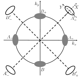
Figure 1: Minima of the fluctuation spectrum $\varepsilon_{\mathbf{k}}$ for the two-dimensional model with square symmetry. The filled (open) ellipses indicate the locations of the lowest energy fluctuations for $\eta>1$ ($\eta<1$). Note that in the isotropic model ($\eta=1$), there is an infinity of degenerate minima located on the circle (solid line).

In the pure paramagnetic limit, the in-plane magnetic field $\mathbf{H}=H_{\parallel}\mathbf{e}_{x}$ only acts on the spins. Hence one can set $A_{i}=0$ in the MGL functional Eq.(1) and use the spectrum Eq.(2) to describe the superconducting fluctuations in the normal state. By increasing $H_{\parallel}$ and lowering the temperature, one may tune the thin film near the tricritical point where $g=0$. The parameter $g$ may change sign, thereby indicating an instability towards the inhomogeneous FFLO state when $g$ is positive.

Furthermore the square symmetry implies $g_{x}=g_{y}=g$, $\gamma_{xx}=\gamma_{yy}=\gamma$ and $\gamma_{xy}=\gamma_{yx}=\eta\gamma$ in Eq.(2). Isotropy is only restored when $\eta=1$ which corresponds to a circular Fermi surface konschelle.press . Then the low energy modes are located around the whole circle defined by $\mathbf{k}^{2}=q_{0}^{2}=g/2\gamma$ in reciprocal space, according to Eq.(5). In the general case ($\eta\neq 1$), the quartic terms $\gamma_{ij}k_{i}^{2}k_{j}^{2}$ introduce a non trivial anisotropy, and the lowest energy are realized around isolated points of the reciprocal state (Fig.1).

The paraconductivity $\sigma_{xx}=\sigma_{yy}$ near the FFLO transition ($g>0$) is obtained from Eq.(19) where the integral extends over the whole reciprocal space. Nevertheless due to the denominator $\varepsilon_{\mathbf{k}}^{3}$ in Eq.(19), the main contribution comes from the lowest energy fluctuation modes.

We shall first identify these isolated minima $\mathbf{k}_{\min}$ of the energy by solving $\partial\varepsilon_{\mathbf{k}}/\partial k_{x}(\mathbf{k}_{\min})=\partial\varepsilon_{\mathbf{k}}/\partial k_{y}(\mathbf{k}_{\min})=0$. The location of these minima differs in the cases $\eta>1$ and $\eta<1$ respectively (Fig.1). In the case $\eta>1$, the spectrum $\varepsilon_{\mathbf{k}}$ has four minima located along the $x$ and $y$ axis, namely at points $A_{\pm}\left(\pm q_{0},0\right)$ and $B_{\pm}\left(0,\pm q_{0}\right)$ of the reciprocal space (Fig.1). Near the minima $A_{\pm}$ located along the $x$ axis, we find that the spectrum can be approximated by

$$\varepsilon_{\mathbf{k}}^{(A_{\pm})}\approx\tau+2g\left(k_{x}\mp q_{0}\right)^{2}+g\left(\eta-1\right)k_{y}^{2}$$ (20)

with $\tau=\alpha-g^{2}/4\gamma=a\left(T-T_{c}\right)$. The expression for the FFLO critical temperature $T_{c}$ coincides with Eq.(6) as long as $\eta>1$.

Similarly, the spectrum around the minima $B_{\pm}\left(0,\pm q_{0}\right)$ located along the $y$ axis is given by

$$\varepsilon_{\mathbf{k}}^{(B_{\pm})}\approx\tau+g\left(\eta-1\right)k_{x}^{2}+2g\left(k_{y}\mp q_{0}\right)^{2}.$$ (21)

The next step consists in evaluating the generalized velocities around each minima. For instance around $A_{+}$, we obtain

$$v_{\mathbf{k}x} =\frac{\partial\varepsilon_{\mathbf{k}}^{(A_{+})}}{\partial k_{x}}=4g\left(k_{x}-q_{0}\right),$$ (22)

$$v_{\mathbf{k}y} =\frac{\partial\varepsilon_{\mathbf{k}}^{(A_{+})}}{\partial k_{y}}=2g\left(\eta-1\right)k_{y}.$$ (23)

Finally, we evaluate the integral Eq.(19) around the minimum $A_{+}$.

Reproducing this steps for the other minima $A_{-},B_{+}$ and $B_{-}$ and summing the contributions from the four minima, one obtains the paraconductivity

$$\sigma_{xx}=\sigma_{yy}=\frac{e^{2}ak_{B}}{4\sqrt{2}\hslash}\frac{1+\eta}{\sqrt{\eta-1}}\left(\frac{T_{c}}{T-T_{c}}\right)\text{.}$$ (24)

which diverges at the FFLO transition.

The second case $\eta<1$ can be treated along the same line of reasoning, albeit the four degenerate minima $\mathbf{k}_{\min}^{\prime}=(k_{\min x}^{\prime},k_{\min y}^{\prime})$ are now located on the diagonals with $(k_{\min x}^{\prime})^{2}=(k_{\min y}^{\prime})^{2}=q_{0}^{2}/2$ (Fig.1). The spectrum can be expanded as

$$\varepsilon_{\mathbf{k}}\approx\tau-{\textstyle\sum\limits_{i,j=x,y}}\lambda_{ij}\left(k_{i}-k_{\min i}^{\prime}\right)\left(k_{j}-k_{\min j}^{\prime}\right),$$ (25)

around any of those four minima denoted $A_{+}^{\prime},A_{-}^{\prime},B_{+}^{\prime}$ and $B_{-}^{\prime}$ (Fig.1), with $\tau=\alpha-g^{2}/2\gamma\left(1+\eta\right)=a\left(T-T_{c}\right)$. For instance, we find

$$\lambda_{xx}=\lambda_{yy}=\frac{2g}{1+\eta}\text{ \ and \ }\lambda_{xy}=\lambda_{yx}=\frac{2g\eta}{1+\eta}$$ (26)

around $A_{+}^{\prime}(q_{0}/\sqrt{2},q_{0}/\sqrt{2})$. Diagonalization of the tensor $\lambda_{ij}$ leads to the eigenvalues $\lambda_{X}=2g$ and $\lambda_{Y}=2g\left(1-\eta\right)/\left(1+\eta\right)$ along the principal axis $X$ and $Y$.

Finally summation over the four minima (Fig.1) yields:

$$\sigma_{xx}=\sigma_{yy}=\frac{e^{2}ak_{B}}{2\hslash}\frac{g^{2}\eta^{2}}{\left(1+\eta\right)^{3}}\sqrt{\frac{1+\eta}{1-\eta}}\left(\frac{T_{c}}{T-T_{c}}\right).$$ (27)

Note that in this regime $\eta<1$, the expression for the FFLO critical temperature $T_{c}$ differs slightly from Eq.(6).

The above expressions Eqs.$\left(\ref{EQ_square_example_out_of_diagonals}\text{,}\ref{EQ_square_example_on_diagonals}\right)$ both diverge for $\eta\rightarrow 1$, which indicates stronger Gaussian fluctuations in the isotropic model konschelle.press .

III.2 Orbital effect associated with an in-plane magnetic field

We now take into account the orbital effect associated with the in-plane magnetic field ($\mathbf{H}=H_{\parallel}\mathbf{e}_{x}$), and show that it breaks the square symmetry, inducing distinct paraconductivities along $x$ and $y$ directions.

In the case of thin films with a strong confinement in the $z$ direction, this orbital effect is small. Then it is still possible to describe the fluctuations by the spectrum Eq.(2) with $H_{\parallel}$-dependent coefficients buzdin_matsuda_shibauchi.2007 , namely by

$$\varepsilon_{\mathbf{k}}=\alpha-g\left(k^{2}+\dfrac{\left(H_{\parallel}d\right)^{2}}{12\Phi_{0}^{2}}\right)+\gamma\left(k^{4}+\dfrac{\left(H_{\parallel}d\right)^{4}}{80\Phi_{0}^{4}}\right)+\\ +2\gamma\left(\eta-1\right)k_{x}^{2}k_{y}^{2}+\dfrac{\left(H_{\parallel}d\right)^{2}}{6\Phi_{0}^{2}}\left(\gamma\eta k_{x}^{2}+3\gamma k_{y}^{2}\right),$$ (28)

where $k^{2}=k_{x}^{2}+k_{y}^{2}$, $d$ is the width of the film along the $z$-axis, and $\Phi_{0}=h/2e$ is the superconducting quantum of flux. Owing to the smallness of the dimensionless parameter $(H_{\parallel}\xi d/q_{0}\Phi_{0})^{2}$, it is still possible to use Eq.(19) in order to evaluate the paraconductivity tensor following the same procedure than in the previous section III.1. Here $\xi$ is the superconducting coherence length.

Due to the field ($H_{\parallel}$) dependence of the coefficients in Eq.(28), the minima of $\varepsilon_{\mathbf{k}}$ are displaced (in comparison to the case $H_{\parallel}\xi d/q_{0}\Phi_{0}=0$ shown in Fig. 1) according to ($\eta>1$):

$$A_{\pm} \rightarrow A_{\pm}\left(\pm\sqrt{\frac{g}{2\gamma}-\frac{\eta\left(H_{\parallel}d\right)^{2}}{12\Phi_{0}^{2}}},0\right),$$ (29)

$$B_{\pm} \rightarrow B_{\pm}\left(0,\pm\sqrt{\frac{g}{2\gamma}-\frac{\left(H_{\parallel}d\right)^{2}}{4\Phi_{0}^{2}}}\right).$$ (30)

Moreover the square symmetry is broken since the critical temperature associated with modulation $A_{\pm}$ differs from the one for $B_{\pm}$. It happens that the FFLO modulation occurs along the field (points $A_{\pm}$) for $\eta<3$. In contrast for $\eta>3$ the modulation occurs along the $y$-axis (points $B_{\pm}$) which is perpendicular to the applied field buzdin_matsuda_shibauchi.2007 .

We concentrate on the case for $1<\eta<3$ wherein the order parameter is modulated along the field $\mathbf{H}=H_{\parallel}\mathbf{e}_{x}$. The paraconductivity comes from the contributions around the points $A_{+}$ and $A_{-}$. Then the paraconductivity $\sigma_{xx}$ measured along the field differs from the one $\sigma_{yy}$ measured in the perpendicular direction. As a main result of this section, the ratio $\sigma_{xx}/\sigma_{yy}$ contains a contribution which diverges at the FFLO transition ($g>0$)

$$\left(\frac{\sigma_{xx}}{\sigma_{yy}}\right)=1+\frac{\gamma}{6g}\left(\frac{H_{\parallel}d}{\Phi_{0}}\right)^{2}\left[\frac{\eta-3}{\eta-1}+\frac{g^{2}}{2\gamma\tau}\frac{(\eta-3)^{2}}{\eta+1}\right].$$ (31)

This term produces a strong enhancement of  $\sigma_{xx}/\sigma_{yy}$ when the transition is approached, namely when $\tau=a\left(T-T_{c}\right)\rightarrow 0^{+}$. This is in sharp contrast with the transition towards a uniform BCS state. There the ratio of the paraconductivities

$$\left(\frac{\sigma_{xx}}{\sigma_{yy}}\right)_{BCS}=1-\frac{\gamma\left(\eta-3\right)}{6g}\left(\frac{H_{\parallel}d}{\Phi_{0}}\right)^{2}$$ (32)

does not contain any divergent term at the BCS transition ($g<0$). Such an enhancement of $\sigma_{xx}/\sigma_{yy}$ may serve as an experimental signature of the FFLO state. This property is reminiscent of the recent finding that critical current oscillates as a function of magnetic orientation in anisotropic 2D films buzdin_matsuda_shibauchi.2007 .

III.3 Orbital effect in a perpendicular magnetic field

Finally, we discuss the effect of a perpendicular component $H_{\perp}\boldsymbol{e}_{z}$ when the field $\mathbf{H}=H_{\parallel}\boldsymbol{e}_{x}+H_{\perp}\boldsymbol{e}_{z}$ is tilted out of the film plane. The perpendicular component $H_{\perp}\boldsymbol{e}_{z}$ quantizes the in-plane motion of the fluctuating Cooper pairs, and induces a finite magnetization. This effect is larger than  the orbital motion associated with the in-plane part of the field. We therefore neglect the later (which is correct for $H_{\parallel}\xi d\ll\Phi_{0}$) and use the MGL functional Eq.(1) within the gauge $A_{x}=0$ and $A_{y}=xH_{\perp}$, like in section II.C.

In the anisotropic case, the eigenmodes of this functional are not known exactly for finite $H_{\perp}$ precluding an analytical evaluation of the magnetization. Nevertheless the isotropic model already exhibits oscillations of the fluctuation magnetization. Recently the fluctuational magnetization (persistent current) of small rings made of a FFLO superconductor was obtained within the framework of the isotropic model introduced in Sec. II.C. In the following, we derive a simple formula for the magnetization in the simpler planar geometry of superconducting films zyuzin09 .

The fluctuation spectrum is given by Eq.(14) and the free energy per unit surface by Eq. (18) with $H=H_{\perp}$. The particular form Eq.(14) of the spectrum enables both degeneracies between the Landau levels ($E_{n}=E_{n+1}$) and commensurability effects between the wavevectors $Q_{n}$ and $q_{0}$.

Single mode (high fields) approximation: For large perpendicular field, namely $H_{\perp}/\Phi_{0}\gg$ $\sqrt{\tau/\gamma}$, the Landau levels are well separated from each others and the main contribution to the free energy Eq.$\left(\ref{F2D}\right)$ comes either from the single level with minimal energy $E_{n}$, or from two levels when a degeneracy ($E_{n}=E_{n+1}$) occurs.

Let us first consider the non-degenerate case. Then the free energy is simply given by the single level contribution

$$F_{n}=\frac{H_{\perp}}{\Phi_{0}}k_{B}T\ln\frac{E_{n}(k_{z}=0)}{\pi k_{B}T}$$ (33)

and the corresponding orbital magnetization (per unit surface)

$$M_{n}=-\frac{(8n+4)k_{B}T}{\Phi_{0}^{2}}\left(\frac{\gamma(Q_{n}^{2}-q_{0}^{2})}{\tau+\gamma(Q_{n}^{2}-q_{0}^{2})^{2}}\right)H_{\perp}$$ (34)

is highly nonlinear since the prefactor of $H_{\perp}$ depends strongly on the field and on temperature. Importantly the magnetization may change sign due to the presence of the factor $Q_{n}^{2}-q_{0}^{2}$ in the numerator. In order to make more transparent the formula Eq.$\left(\ref{Eq_Msingle}\right)$, one may introduce the field-dependent temperature $T_{cn}(H)$ where the denominator vanishes:

$$a(T-T_{cn})=\tau+\gamma(Q_{n}^{2}-q_{0}^{2})^{2}$$ (35)

This relation defines the second-order transition line $T_{c}^{(n)}(H)$ between the normal and the modulated superconducting state described by the $n$-th Landau level. We also define the points like A,C,E (Fig.2) along this transition line where the numerator vanishes since $Q_{n}^{2}=q_{0}^{2}$. Those points are also located on the second-order transition line $T_{cP}(H)$ between the normal and the FFLO superconducting state calculated in the pure paramagnetic limit. In the normal state, the orbital magnetization can be therefore reexpressed as

$$M_{n}=-\frac{(8n+4)k_{B}T}{\Phi_{0}^{2}}\frac{\gamma}{a}\left(\frac{Q_{n}^{2}-q_{0}^{2}}{T-T_{cn}}\right)H_{\perp}$$ (36)

This 2D magnetization is diamagnetic when $Q_{n}^{2}>q_{0}^{2}$ and paramagnetic when $Q_{n}^{2}<q_{0}^{2}$ (Fig.2). In contrast, the fluctuation magnetization is always diamagnetic in the BCS case. However $M_{n}$ follows a similar power law $(T-T_{c}^{(n)})^{-1}$ and is on the same order of magnitude than the BCS magnetization b.larkin_varlamov . Consequently we expect that the oscillations between diamagnetism and paramagnetism should be measurable in thin films of FFLO superconductors. This single mode approximation breaks down when the $n$-th and ($n+1$)-th Landau levels are degenerate, namely when $E_{n}=E_{n+1}$. Then the two levels must be included together in the free energy, whereas the other Landau levels are still far in energy and can be neglected safely. The resulting magnetization $M_{n}+M_{n+1}$ is slightly diamagnetic at degeneracy.

Continuum (low fields) approximation: The single mode approximation breaks down in the weak field limit ($H_{\perp}/\Phi_{0}\ll$ $\sqrt{\tau/\gamma}$) where the Landau level separation becomes so small that all the levels have to be taken into account. This situation corresponds to a magnetic field which is slightly tilted out of the film plane. In the case of a uniform BCS superconductor, the standard result for the magnetization is schmid.1969 :

$$M=\frac{\pi}{3}\frac{k_{B}T}{\Phi_{0}^{2}}\frac{g}{a(T-\tilde{T}_{c})}H_{\perp}$$ (37)

which is diamagnetic ($g<0$) and diverges at the BCS critical temperature $\tilde{T}_{c}\left(H\right)$ for the second order phase transition. This diamagnetic response is suppressed when the tricritical point is approached, i.e. when $g\rightarrow 0^{-}$ (Fig.2)konschelle.press . On the FFLO side (region $g>0$ in Fig.2) and for a given magnetic field, the system becomes a FFLO superconductor before the divergency develops because $T_{c}>\tilde{T}_{c}$.

Conclusion: At high fields $H_{\perp}$, the magnetization near the FFLO transition line oscillates between sizeable diamagnetism and paramagnetism as the transitions between successive Landau levels are realized. In the low field limit, these transitions become very close and the oscillations average themselves leading to a cancellation of the linear response and a suppression of the divergency. This situation is in strong contrast with the standard BCS case where the magnetization is always diamagnetic. We suggest to perform magnetization measurements in thin films near an expected FFLO transition. The suppression of the fluctuational magnetization at low perpendicular field and the restoration of sizeable oscillations between para- and diamagnetism at higher perpendicular field should be a strong indication for the FFLO state in quasi-two dimensional compounds.

IV Anisotropic 3D superconductors

It is commonly believed that the FFLO state in CeCoIn₅ corresponds to a modulation along the applied magnetic field. Nevertheless it was argued recently that this situation is unlikely to happen for arbitrary field orientations when the tetragonal anisotropy of CeCoIn₅ is properly taken into account. Apparently if the order parameter modulation is along the field for $\mathbf{H\perp c}$ (resp. $\mathbf{H\parallel c}$), then the modulation is likely to be perpendicular to the field for $\mathbf{H\parallel c}$ (resp. $\mathbf{H\perp c}$) denisov09 . Here we investigate the FFLO fluctuations in anisotropic 3D compounds, building upon the various mean-field scenarios reported in Refdenisov09 . We evaluate the fluctuational magnetization $M$ along the magnetic field $\mathbf{H}=H\mathbf{e}_{z}$. In particular, we demonstrate below that the magnetization oscillates between sizeable diamagnetism and paramagnetism when the modulation is perpendicular to the field (Landau level like). Those oscillations are the 3D counterparts of the ones predicted in the previous section for superconducting films. In contrast the magnetization is shown to be strongly suppressed when the modulation occurs along the field (FFLO like modulation). In the 3D case, magnetization measurements therefore provide an experimental tool to discriminate between the two possible order parameter structures uncovered in Refdenisov09 .

IV.1 Mean field

We start by a short reviewing of the mean-field properties of the functional

$$H =\alpha\left|\Psi\right|^{2}-\sum_{i=x,y,z}g\left|D_{i}\Psi\right|^{2}+\gamma\left|\sum_{i=x,y,z}D_{i}^{2}\right|^{2}$$

$$+\varepsilon_{z}\left|D_{z}^{2}\Psi\right|^{2}+\varepsilon_{x}(\left|D_{x}D_{y}\Psi\right|^{2}+\left|D_{y}D_{x}\Psi\right|^{2})$$

$$+\varepsilon(\left|D_{x}D_{z}\Psi\right|^{2}+\left|D_{z}D_{x}\Psi\right|^{2})$$

$$+\varepsilon(\left|D_{y}D_{z}\Psi\right|^{2}+\left|D_{z}D_{y}\Psi\right|^{2})$$ (38)

consistent with the tetragonal symmetry of CeCoIn₅. The terms $\varepsilon_{z},$ $\varepsilon_{x}$ and $\varepsilon$ describe nontrivial (namely different from a simple elliptical) anisotropy denisov09 . Note that the cubic symmetry corresponds to $\varepsilon_{x}=\varepsilon$ and $\varepsilon_{z}=0$. It was shown that two kinds of modulated superconducting states (scenarios a) and b) mentioned above in the general introduction) are the most likely to occur when anisotropies are properly taken into account.

The class a) of solutions corresponds to order parameters modulated along the field with characteristic FFLO wave-vector $q_{0}$ and in the $n=0$ Landau level. Following the mean field analysis of Refdenisov09 , we write the fluctuation spectrum as

$$E_{n=0}(k_{z})=\tau+\gamma_{a}\left(\dfrac{2eH}{\hslash}+k_{z}^{2}-q_{0}^{2}\right)^{2}$$ (39)

which indicates an instability towards finite modulation along the $z$ axis (magnetic field). This is similar than Eq.(14) except that the Landau index is fixed $n=0$ and $\gamma_{a}$ is a renormalized parameter (specific to this class a) of solutions) which depends on $\varepsilon_{z},$ $\varepsilon_{x}$ and $\varepsilon$.

In the class b) of solutions, the modulation occurs in the plane perpendicular to the field and is described by a higher ($n>0$) Landau level. Following the mean field analysis of Refdenisov09 , we write the fluctuation spectrum as

$$E_{n}(k_{z})=\tau+\gamma_{b}(Q_{n}^{2}-q_{0}^{2})^{2}+g_{b}k_{z}^{2}.$$ (40)

This spectrum differs from Eq.$\left(\ref{spectrumclassa}\right)$ since the kinetic energy term $g_{b}k_{z}^{2}$ favors $k_{z}=0$. Furthermore a finite Landau index is possible, since the energy is also minimized by choosing $n$ such as $Q_{n}^{2}-q_{0}^{2}\sim 0$. In brief, the lowest energy fluctuations in the normal state ressemble the superconducting groundstate which is modulated perpendicularly to the field. Note that here $\gamma_{b}$ and $g_{b}$ are also renormalized parameters which are specific to the class b) of solutions and depend on $\varepsilon_{z},$ $\varepsilon_{x}$ and $\varepsilon$ in a complicated manner denisov09 .

IV.2 Fluctuation magnetization

Here we evaluate the magnetization induced by the FFLO fluctuations taking into account the intrinsic anisotropy present in 3D compounds. The FFLO transition might happen under low or strong field, depending on the underlaying microscopic mechanism. For instance, in the rare earth magnetic superconductor ErRh₄B₄ a small field is sufficient to polarize the internal moments, and the FFLO transition is thus expected at low applied magnetic field bulaevskii85 . Here we treat the case of the FFLO transition occuring under strong magnetic field which is relevant for the case of the heavy fermion superconductor CeCoIn₅. Using a single Landau level approximation, we demonstrate that the magnetization exhibits qualitatively distinct behaviors depending on the class of solutions.

FFLO-like modulation along the field, characterized by a finite wave-vector $q_{0}$ and Landau index $n=0$ (scenario a) discussed in the introduction). The 3D density of free energy is given by the integral

$$F=k_{B}T\frac{H}{\Phi_{0}}\int\frac{dk_{z}}{2\pi}\ln\frac{E_{n=0}(k_{z})}{\pi k_{B}T}$$ (41)

where the energy $E_{n=0}(k_{z})$ is given by Eq.$\left(\ref{spectrumclassa}\right)$. Hence the most divergent part of the orbital magnetization (per unit volume) $M=-\partial F/\partial H$ is given by

$$M =-\frac{2k_{B}T}{\Phi_{0}^{2}}\times$$

$$\times\left(\int_{-\infty}^{\infty}dk_{z}\frac{\gamma_{a}\left(2eH/\hslash+k_{z}^{2}-q_{0}^{2}\right)}{\tau+\gamma_{a}\left(2eH/\hslash+k_{z}^{2}-q_{0}^{2}\right)^{2}}\right)H,$$ (42)

where $\Phi_{0}=h/(2e)$. Since the numerator of the integrand cancels and changes sign as a function of $k_{z}$, one expects a strong suppression of the fluctuation magnetization compared to the uniform BCS case wherein such a cancellation does not occur. Indeed the magnetization $M$ diverges logarithmically at the FFLO transition which is less divergent than the $\tau^{-1/2}$ law predicted in the standard BCS case. Therefore the presence of a genuine FFLO state should be detected as a suppression of the fluctuation diamagnetism observed near the BCS transition. In comparison with the 2D case, the oscillations between paramagnetism and diamagnetism predicted in the previous section are blurred out by the dispersion over the momentum $k_{z}$ along the field.

Landau level modulation perpendicular to the field (scenario b) discussed in the introduction). The dispersion of the fluctuations Eq.$\left(\ref{spectrumclassb}\right)$ now favors the absence of modulation along the $z$ axis in contrast to the spectrum Eq.(39). Upon increasing the parameter $q_{0}^{2}$, the lowest energy Landau level is successively $n=0$, then $n=1$ etc… Near the BCS transition ($g>0$), the fluctuations induce diamagnetism and a lowering of the critical field $H_{c2}(T)$ below the purely paramagnetic critical field $H_{P}(T)$ at the same temperature (Fig.2). When the $n$-th Landau level is realized and when all the other Landau levels are distant in energy, one can single out the contribution of this main level to the density of free energy

$$F=k_{B}T\frac{H}{\Phi_{0}}\int_{-\infty}^{\infty}\frac{dk_{z}}{2\pi}\ln\frac{\tau+\gamma_{b}(Q_{n}^{2}-q_{0}^{2})^{2}+g_{b}k_{z}^{2}}{\pi k_{B}T}.$$ (43)

Writing the orbital magnetization as

$$M_{n} =-\frac{(4n+2)k_{B}T}{\Phi_{0}^{2}}\times$$

$$\times\left(\int_{-\infty}^{\infty}dk_{z}\frac{\gamma_{b}(Q_{n}^{2}-q_{0}^{2})}{\tau+\gamma_{b}(Q_{n}^{2}-q_{0}^{2})^{2}+g_{b}k_{z}^{2}}\right)H_{\perp},$$ (44)

shows that the 2D oscillations are no longer suppressed by the integration over $k_{z}$ since the numerator is independent of $k_{z}$. Calculating the integral shows that the magnetization diverges as

$$M_{n}=-\frac{(4n+2)k_{B}T}{\Phi_{0}^{2}}\frac{\gamma_{b}}{\left(ag_{b}\right)^{1/2}}\frac{Q_{n}^{2}-q_{0}^{2}}{\left(T-T_{cn}\right)^{1/2}}H_{\perp}$$ (45)

with the same power law than in the BCS transition of 3D superconductors b.larkin_varlamov . Unlike the BCS case, this fluctuation magnetization changes sign being diamagnetic when $Q_{n}^{2}>q_{0}^{2}$ (arcs $BC$, $DE$ in Fig.2) and paramagnetic when $Q_{n}^{2}<q_{0}^{2}$ (arcs $AB$, $CD$).

In brief, the magnetization is sizeable and oscillates between para- and diamagnetism when the superconducting order parameter is modulated perpendicularly to the field, whereas it is strongly suppressed when the order parameter is modulated along the field. Therefore magnetization measurements may serve as a test to discriminate between FFLO and Landau level like modulations in 3D anisotropic superconductors.

Figure 2: Schematic field-temperature $\left(H,T\right)$ phase diagram showing the cascade of Landau levels. The thick dashed curve represents the critical field in the absence of orbital effect. In presence of orbital effect, the critical field is reduced and described by the thin dashed curves which corresponds respectively to the $n=0,$ $n=1$ and $n=2$ Landau levels. The solid line represents schematically the expected transition line between the normal and the superconducting states. The fluctuations are diamagnetic between zero field ($H=0,T_{c}$) and $B$, paramagnetic near the arc $AB$, then again diamagnetic near the arc $BC$, etc…The Landau levels are degenerate at points $B$,$D$, etc… This schematic picture is relevant for both 2D FFLO superconductors and for 3D ones where the Landau level modulation is realized (scenario b) evoked in the introduction).

V Conclusion.

We investigated the conductivity and the orbital magnetization associated with superconducting fluctuations above the FFLO critical temperature or field. Both in 2D and 3D models, we shown that these properties differ considerably than their counterparts at the vicinity of a standard BCS transition towards an homogeneous superconducting state, thereby providing an experimental tool to detect the inhomogeneous state. First, the paraconductivity of thin superconducting films exhibits a strong anisotropy when measured parallel or perpendicular to the FFLO modulation. Second, the orbital magnetization oscillates between diamagnetic and paramagnetic behaviors at high fields, and is strongly suppressed at low fields, whereas the uniform BCS state always induces diamagnetic fluctuations above $T_{c}$. We suggest performing magnetization and conductance measurements along the FFLO transition line in compounds where the FFLO state has been recently reported. In 2D organic superconductors uji.2006 ; lortz.2007 , the magnetization oscillations should be even more pronounced than in the 3D magnetic superconductors (ErRh₄B₄ , see bulaevskii85 ) or in the case of the anisotropic 3D heavy fermion superconductor CeCoIn₅radovan03 ; bianchi02 ; bianchi03 . It was recently shown that CeCoIn₅ has quasi-2D Fermi-surface sheets coexisting with a 3D anisotropic Fermi surface ko . Nevertheless due to strong hybridization, superconductivity in CeCoIn₅ is likely to be described by a single order parameter. The complex structure of the Fermi surface should only modify the expressions of the coefficients in the MGL functional as functions of the microscopic parameters of CeCoIn₅. Moreover, the fact that the Landé factor is anisotropic leads to different Maki parameters depending on the field orientation and may also shift the position of the tricritical point shimahara_matsuda . Nevertheless the magnetization oscillations/suppression predicted here are generic of the presence of FFLO phase, and should pertain independently of the microscopic characteristics of CeCoIn₅.

Finally, in the 3D case, we find that the absence of such oscillations reveals a FFLO state modulated along the field whereas presence of oscillations should be associated with a multiquanta Landau modulation perpendicular to the field.

VI APPENDIX

In this appendix, we address the validity of the Gaussian approximation used in this paper. When the temperature is sufficiently close to the critical one, interactions between the fluctuation modes become so strong that the Gaussian approximation breaks down. In order to quantify the range of temperature where this breakdown occurs, we derive the Ginzburg-Levanyuk criterion for the FFLO transition b.landau.V_e ; levanyuk.1959 ; ginzburg.1960 .

VI.1 Ginzburg-Levanyuk criterion for the FFLO transition

The full isotropic MGL functional $H\left[\Psi\right]=H_{G}\left[\Psi\right]+H_{int}[\Psi]$ contains a quadratic part

$$H_{G}\left[\Psi\right] =N_{d}(0)\int d\boldsymbol{r}\left[\widetilde{\alpha}\left|\Psi\right|^{2}-\widetilde{g}\xi^{2}\left|\partial\Psi\right|^{2}+\xi^{4}\left|\partial^{2}\Psi\right|^{2}\right]$$ (46)

$$=N_{d}(0)\sum_{\mathbf{k}}\left(\widetilde{\tau}+(\mathbf{k}^{2}-q_{0}^{2})^{2}\xi^{4}\right)$$ (47)

which describes the free dynamics of the order parameter $\Psi,$ and non quadratic terms $H_{int}[\Psi]$ which describe interactionsbuzdin_kachkachi(1997) ; yang_agterberg.2001 ; houzet2006 . All the results of this paper are derived within the Gaussian approximation which consists in using $H_{G}\left[\Psi\right]$ as the free energy functional thereby neglecting completely $H_{int}\left[\Psi\right]$. In the spirit of the original levanyuk.1959 ; ginzburg.1960 and textbookb.landau.V_e Ginzburg-Levanyuk criterion, we evaluate the interaction terms

$$H_{int}\left[\Psi\right]=N_{d}(0)\int d\boldsymbol{r}\left[\frac{\widetilde{g}}{T_{c}^{2}}\left|\Psi\right|^{4}+\frac{1}{T_{c}^{4}}\left|\Psi\right|^{6}\right].$$ (48)

in order to compare them with $H_{G}\left[\Psi\right]$.

We have introduced the dimensionless coefficients $\widetilde{\alpha}=(T-\tilde{T}_{c})/\tilde{T}_{c}$, $\widetilde{\tau}=(T-T_{c})/T_{c}$, and $\widetilde{g}$ to make apparent the order of magnitude of ech term in the MGL functional as a function of the the energy scales $T_{c}$ and $E_{F}$. In particular the dimensionless parameter $\widetilde{g}$ is of order one. We have also introduced the $d$-dimensional electronic density of states $N_{d}(0)$ and the superconducting coherence length $\xi=v_{F}/T_{c}$ (we set $\hslash=1$). Here $q_{0}^{2}=\widetilde{g}/2\xi^{2}$ in analogy with the transformation performed in Eq. (5). It is a rather particular property of the MGL functional that the coefficients of the $\left|\Psi\right|^{4}$ and $\left|\partial\Psi\right|^{2}$ vanish at the same point $(H,T)$ of the phase diagram (the tricritical point) buzdin_kachkachi(1997) . For this reason and since we are solely interested in orders of magnitude here, we have denoted the coefficient of the $\left|\Psi\right|^{4}$ term by the same $\widetilde{g}$ used for the $\left|\partial\Psi\right|^{2}$.

For examples of phase transitions, one usually evaluates only the $\left|\Psi\right|^{4}$ terms b.landau.V_e . Here the situation of the FFLO transition is rather specific since on the line $\widetilde{g}=g=0$ of the $(T,H)$ phase diagram the coefficient of the $\left|\Psi\right|^{4}$ term vanishes. Therefore one should evaluate the next interacting term, $\left|\Psi\right|^{6}$, for the regions near this line $\widetilde{g}=0$. Sufficiently far away from this line $\widetilde{g}=0$ (see the quantitative criterion below), one may simply evaluate the $\left|\Psi\right|^{4}$ term.

Using Wick theorem to evaluate $H_{int}\left[\Psi\right]=H_{int}^{(4)}\left[\Psi\right]+H_{int}^{(6)}\left[\Psi\right]$, we find

$$H_{int}^{(4)}\left[\Psi\right]=\frac{2\widetilde{g}N_{d}(0)}{T_{c}^{2}L^{d}}\sum_{\mathbf{k,k}^{\prime}}\left\langle\left|\Psi_{\mathbf{k}}\right|^{2}\right\rangle_{0}\left\langle\left|\Psi_{\mathbf{k}^{\prime}}\right|^{2}\right\rangle_{0}$$ (49)

for the $\left|\Psi\right|^{4}$ term, and

$$H_{int}^{(6)}\left[\Psi\right]=N_{d}(0)\sum_{\mathbf{k}}\left(\frac{2}{T_{c}^{2}L^{d}}\sum_{\mathbf{k}^{\prime}}\left\langle\left|\Psi_{\mathbf{k}^{\prime}}\right|^{2}\right\rangle_{0}\right)^{2}\left\langle\left|\Psi_{\mathbf{k}}\right|^{2}\right\rangle_{0},$$ (50)

for the $\left|\Psi\right|^{6}$ term. Note that in this problem the form of the free field correlator

$$\left\langle\left|\Psi_{\mathbf{k}}\right|^{2}\right\rangle_{0}=\frac{\pi k_{B}T_{c}/N_{d}(0)}{\widetilde{\tau}+\xi^{4}\left(k^{2}-q_{0}^{2}\right)^{2}}.$$ (51)

is rather special due to the proximity of the FFLO transition.

VI.2 Isotropic model

Far from the tricritical point, namely when $\widetilde{g}\geqslant(T_{c}/E_{F})^{2(d-1)/(6-d)}$, the leading correction to the Gaussian behavior originates from the $\left|\Psi\right|^{4}$ interaction term. Morover the fluctuations propagate with a quadratic dispersion, and the correlator Eq.(51) can be approximated as

$$\left\langle\left|\Psi_{\mathbf{k}}\right|^{2}\right\rangle_{0}=\frac{\pi k_{B}T_{c}/N_{d}(0)}{\widetilde{\tau}+4q_{0}^{2}\xi^{4}\left(k-q_{0}\right)^{2}}$$ (52)

when evaluating the sum

$$\frac{\widetilde{g}}{T_{c}^{2}L^{d}}\sum_{\mathbf{k}^{\prime}}\left\langle\left|\Psi_{\mathbf{k}^{\prime}}\right|^{2}\right\rangle_{0}=\frac{\widetilde{g}^{d/2}\widetilde{\tau}^{-1/2}}{T_{c}N_{d}(0)\xi^{d}}.$$ (53)

Using $T_{c}N_{d}(0)\xi^{d}=(E_{F}/T_{c})^{d-1}$, we find that the $\left|\Psi\right|^{4}$ interaction terms are negligible in comparison to the Gaussian ones when the condition (Ginzburg-Levanyuk criterion)

$$\widetilde{\tau}\gg\widetilde{g}^{d/3}\left(\frac{T_{c}}{E_{F}}\right)^{2(d-1)/3}$$ (54)

is fullfilled. The critical region width is larger than in the standard BCS case ($\tau\gg\left(T_{c}/E_{F}\right)^{4}$ for $d=3$ and $\widetilde{\tau}\gg T_{c}/E_{F}$ for $d=2$) but it remains extremelly thin.

Near the tricritical point, when $\widetilde{g}\leqslant(T_{c}/E_{F})^{2(d-1)/(6-d)}$, the $\left|\Psi\right|^{6}$ interaction becomes stronger than the $\left|\Psi\right|^{4}$ one since this latter contribution is suppressed by the extremelly small prefactor $\widetilde{g}$. In particular, along the $\widetilde{g}=g=0$ line in the ($H,T$) diagram, the $\left|\mathbf{\nabla}\Psi\right|^{2}$ and $\left|\Psi\right|^{4}$ terms are totally absent from the functional buzdin_kachkachi(1997) . Therefore one should compute the mean value $\left\langle\left|\Psi_{\mathbf{k}}\right|^{2}\right\rangle_{0}$ with a purely quartic momentum dependence. Since

$$\frac{1}{T_{c}^{2}}\frac{1}{N_{d}(0)L^{d}}\sum_{\mathbf{k}^{\prime}}\left\langle\left|\Psi_{\mathbf{k}^{\prime}}\right|^{2}\right\rangle_{0}=\frac{\widetilde{\tau}^{(d-4)/4}}{T_{c}N_{d}(0)\xi^{d}},$$ (55)

the condition to neglect the $\left|\Psi\right|^{6}$ interaction between the fluctuation modes is thus

$$\widetilde{\tau}\gg\left(\frac{T_{c}}{E_{F}}\right)^{4(d-1)/(6-d)}$$ (56)

The critical fluctuations are present in a larger region of the phase diagram than for BCS superconductivity b.larkin_varlamov . During the completion of this work, we became aware of Ref.zyuzin09 where the Ginzburg-Levanyuk criterion is derived by evaluting exclusively the $\left|\Psi\right|^{4}$ interaction term. We therefore obtain the same Ginzburg-Levanyuk criterion as in Ref.zyuzin09 for the large $\widetilde{g}$ regime whereas our criteria differ when approaching the tricritical point. In spite of this discrepancy, both procedures lead to the same practical conclusion that the critical region remains extremelly thin and inaccessible for experimental observations, because of the smallness of the ratio $T_{c}/E_{F}\sim(10^{-2}-10^{-3})$.

VI.3 Anisotropic model.

We now derive the Ginzburg-Levanyuk criterion in the case of anistropic FFLO superconductors. The large $g$ regime is modified in comparison to the isotropic case, since there the low energy fluctuations are located around few isolated points instead being spread over a large shell of radius $q_{0}$.

Far from the tricritical point, namely when $\widetilde{g}\geqslant(T_{c}/E_{F})^{2(d-1)/(6-d)}$, the leading correction to the Gaussian behavior originates from the $\left|\Psi\right|^{4}$ interaction term. Moreover the fluctuations propagate with a quadratic dispersion, and the correlator Eq.(51) can be approximated as

$$\left\langle\left|\Psi_{\mathbf{k}}\right|^{2}\right\rangle_{0}=\frac{\pi k_{B}T_{c}/N_{d}(0)}{\widetilde{\tau}+\widetilde{g}k^{2}\xi^{2}}.$$ (57)

Evaluating the sum

$$\frac{\widetilde{g}}{T_{c}^{2}L^{d}}\sum_{\mathbf{k}^{\prime}}\left\langle\left|\Psi_{\mathbf{k}^{\prime}}\right|^{2}\right\rangle_{0}=\left(\frac{\tau}{\widetilde{g}}\right)^{{}^{(d-2)/2}}\frac{1}{T_{c}N_{d}(0)\xi^{d}}$$ (58)

and using $T_{c}N_{d}(0)\xi^{d}=(E_{F}/T_{c})^{d-1}$, we find that the $\left|\Psi\right|^{4}$ interaction terms are negligible in comparison to the Gaussian ones when the condition (Ginzburg-Levanyuk criterion)

$$\widetilde{\tau}\gg\widetilde{g}^{(2-d)/(4-d)}\left(\frac{T_{c}}{E_{F}}\right)^{2(d-1)/(4-d)}$$ (59)

is fullfilled. This Ginzburg-Levanyuk criterion is similar (same power of $T_{c}/E_{F}$) than the one encountered in the standard BCS case.

Near the tricritical point, when $\widetilde{g}\leqslant(T_{c}/E_{F})^{2(d-1)/(6-d)}$, the lowest energy fluctuations are located around the origin of the reciprocal space and have a quartic dispersion like in the isotropic model studied above. The Ginzburg-Levanyuk criterion is thus again

$$\widetilde{\tau}\gg\left(\frac{T_{c}}{E_{F}}\right)^{4(d-1)/(6-d)}$$ (60)

near the tricritical point.

VI.4 Conclusion

We have obtained that the size of the critical region in FFLO superconductors is more extended than in the usual uniform superconductor case. Nevertheless, for superconducting compounds, the ratio $T_{c}/E_{F}\sim(10^{-2}-10^{-3})$ is small and the critical region thus remains hardly accessible for experimental observations, thereby supporting the Gaussian analysis performed in this paper. This fact makes very difficult the observation of the phenomena (first-order transition) predicted by renormalization group studies brazovskii.1975 ; dalidovich_yang.2004 .

References

- (1) P. Fulde, and R. A. Ferrell. Phys. Rev. 135, A550 (1964).
- (2) A. Larkin, and Y. Ovchinnikov. Sov. Phys. JETP 20, 762 (1965).
- (3) L.N. Bulaevskii et al., Adv. Phys. 34, 175 (1985).
- (4) R. Casalbuoni, and G. Nardulli. Rev. Mod. Phys. 76, 263 (2004).
- (5) Y. Mastuda, and H. Shimahara J. Phys. Soc. Jap. 76, 051005 (2007).
- (6) H. Radovan et al. Nature 425, 51 (2003).
- (7) A. Bianchi et al. Phys. Rev. Lett. 89, 137002 (2002).
- (8) A. Bianchi et al. Phys. Rev. Lett. 91, 187004 (2003).
- (9) S. Uji et al. Phys. Rev. Lett. 96, 157001 (2006).
- (10) R. Lortz et al. Phys. Rev. Lett. 99, 187002 (2007).
- (11) L.W. Gruenberg and L. Gunther, Phys. Rev. Lett. 16, 996 (1966).
- (12) A.I. Buzdin and J.P. Brison, Phys. Lett. A 218, 359 (1996).
- (13) A.I. Buzdin and J.P. Brison, Europhys. Lett. 35, 707 (1996).
- (14) J.P. Brison et al, Physica C 250, 128 (1995).
- (15) K. Yang, and S. Sondhi. Phys. Rev. B 57, 8566 (1998).
- (16) A. Vorontsov, J. Sauls, and M. Graf. Phys. Rev. B 72, 184501 (2005).
- (17) D. Denisov, A. Buzdin, and H. Shimahara, Phys. Rev. B 79, 064506 (2009).
- (18) D. Saint-James, D. Sarma, and E.J. Thomas, Type II superconductivity (Pergamon Press, New-York, 1969).
- (19) A. I. Buzdin, and H. Kachkachi. Phys. Lett. A 225, 341 (1997).
- (20) D. Agterberg, and K. Yang. J. Phys.: Condens. Matter 13, 9259 (2001).
- (21) M. Houzet and V. P. Mineev, Phys. Rev. B 74, 144522 (2006).
- (22) F. Konschelle, J. Cayssol, and A. I. Buzdin, Europhys. Lett. 79, 67001 (2007).
- (23) R. Bel et al., Phys. Rev. Lett. 92, 217002 (2004).
- (24) Y. Onose, Lu Li, C. Petrovic, N. P. Ong, Europhys. Lett. 79, 17006 (2007).
- (25) L. D. Landau, and E. M. Lifshitz. Course of theoretical physics, Volume 5 : Statistical Physics, 3rd edition (Butterworth-Heinemann, 1980).
- (26) M. Tinkham, Introduction to Superconductivity (Mc-Graw Hill, second edition, 1996).
- (27) W.J. Skocpol, and M. Tinkham, Rep. on Prog. Phys. 38, 1049 (1975).
- (28) A. Larkin, and A. Varlamov. The physics of superconductors, Vol. I : Conventional and high- superconductors, chapter 3, Fluctuation phenomena in superconductors (K.H. Bennemann and J.B. Ketterson, Springer-Verlag, 2003).
- (29) A.I. Buzdin, Y. Matsuda, and T. Shibauchi. Europhys. Lett. 80, 67004 (2007).
- (30) A.A. Zyuzin, A.Yu. Zyuzin, arXiv:0901.1562; A.A. Zyuzin, A.Yu. Zyuzin, JETP Lett. 88, 147 (2008).
- (31) This useful property relies on the isotropy of the model treated in Sec. II. In the anisotropic case (Sec. III) is replaced by a more complicated operator whose eigenmodes differ from the ones of and are not known exactly.
- (32) L. D. Landau, and E. M. Lifshitz. Course of theoretical physics, Volume 3 : Quantum Mechanics, 3rd edition (Butterworth-Heinemann, 2001).
- (33) A. Schmid. Phys. Rev. 180, 527 (1969).
- (34) A. Koitzsch et al., Phys. Rev. B 79, 075104 (2009).
- (35) A. Levanyuk. Sov. Phys. JETP 36, 571 (1959).
- (36) V. L. Ginzburg. Sov. Solid State 2, 61 (1960).
- (37) S. A. Brazovskii. Sov. Phys. JETP 41, 85 (1975).
- (38) D. Dalidovich, and K. Yang. Phys. Rev. Let. 93, 247002 (2004).