Diffusion-controlled phase growth on dislocations

Abstract

We treat the problem of diffusion of solute atoms around screw dislocations. In particular, we express and solve the diffusion equation, in radial symmetry, in an elastic field of a screw dislocation subject to the flux conservation boundary condition at the interface of a new phase. We consider an incoherent second-phase precipitate growing under the action of the stress field of a screw dislocation. The second-phase growth rate as a function of the supersaturation and a strain energy parameter is evaluated in spatial dimensions $d=2$ and $d=3$. Our calculations show that an increase in the amplitude of dislocation force, e.g. the magnitude of the Burgers vector, enhances the second-phase growth in an alloy. Moreover, a relationship linking the supersaturation to the precipitate size in the presence of the elastic field of dislocation is calculated.

I Introduction

Dislocations can alter different stages of the precipitation process in crystalline solids, which consists of nucleation, growth and coarsening Larché (1979); Wagner and Kampmann (1991). Distortion of the lattice in proximity of a dislocation can enhance nucleation in several ways Porter and Easterling (1981); Christian (2002). The main effect is the reduction in the volume strain energy associated with the phase transformation. Nucleation on dislocations can also be helped by solute segregation which raises the local concentration of the solute in the vicinity of a dislocation, caused by migration of solutes toward the dislocation, the Cottrell atmosphere effect. When the Cottrell atmosphere becomes supersaturated, nucleation of a new phase may occur followed by growth of nucleus. Moreover, dislocation can aid the growth of an embryo beyond its critical size by providing a diffusion passage with a lower activation energy.

Precipitation of second-phase along dislocation lines has been observed in a number of alloys Aaronson et al. (1971); Aaron and Aaronson (1971). For example, in Al-Zn-Mg alloys, dislocations not only induce and enhance nucleation and growth of the coherent second-phase MgZn₂ precipitates, but also produce a spatial precipitate size gradient around them Allen and Vander Sande (1978); Deschamps et al. (1999); Deschamps and Brechet (1999). Cahn Cahn (1957) provided the first quantitative model for nucleation of second-phase on dislocations in solids. In Cahn’s model, it is assumed that a cross-section of the nucleus is circular, which is strictly valid for a screw dislocation Larché (1979). Also, it is posited that the nucleus is incoherent with the matrix so that a constant interfacial energy can be allotted to the boundary between the new phase and the matrix. An incoherent particle interface with the matrix has a different atomic configuration than that of the phases. The matrix is an isotropic elastic material and the formation of the precipitate releases the elastic energy initially stored in its volume. Moreover, the matrix energy is assumed to remain constant by precipitation. In this model, besides the usual volume and surface energy terms in the expression for the total free energy of formation of a nucleus of a given size, there is a term representing the strain energy of the dislocation in the region currently occupied by the new phase. Cahn’s model predicts that both a larger Burgers vector and a more negative chemical free energy change between the precipitate and the matrix induce higher nucleation rates, in agreement with experiment Aaronson et al. (1971); Aaron and Aaronson (1971).

Segregation phenomenon around dislocations, i.e. the Cottrell atmosphere effect, has been observed among others in Fe-Al alloys doped with boron atoms Blavette et al. (1999) and in silicon containing arsenic impurities Thompson et al. (2007), in qualitative agreement with Cottrell and Bilby’s predictions Cottrell and Bilby (1949). Cottrell and Bilby considered segregation of impurities to straight-edge dislocations with the Coulomb-like interaction potential of the form $\phi=A\sin\theta/r$, where $A$ contains the elasticity constants and the Burgers vector, and $(r,\theta)$ are the polar coordinates. Cottrell and Bilby ignored the flow due concentration gradients and solved the simplified diffusion equation in the presence of the aforementioned potential field. The model predicts that the total number of impurity atoms removed from solution to the dislocation increases with time $t$ according to $N(t)\sim t^{2/3}$, which is good agreement with the early stages of segregation of impurities to dislocations, e.g. in iron containing carbon and nitrogen Harper (1951). A critical review of the Bilby-Cottrell model, its shortcomings and its improvements are given in Bullough and Newman (1970).

The object of our present study is the diffusion-controlled growth of a new phase, i.e., a post nucleation process in the presence of dislocation field rather than the segregation effect. As in Cahn’s nucleation model Cahn (1957), we consider an incoherent second-phase precipitate growing under the action of a screw dislocation field. This entails that the stress field due to dislocation is pure shear. The equations used for diffusion-controlled growth are radially symmetric. These equations for second-phase in a solid or from a supercooled liquid have been, in the absence of an external field, solved by Frank Frank (1950) and discussed by Carslaw and Jaeger Carslaw and Jaeger (1959). The exact analytical solutions of the equations and their various approximations thereof have been systematized and evaluated by Aaron et al. Aaron et al. (1970), which included the relations for growth of planar precipitates. Applications of these solutions to materials can be found in many publications, e.g. more recent papers on growth of quasi-crystalline phase in Zr-base metallic glasses Köster et al. (1996) and growth of Laves phase in Zircaloy Massih et al. (2003). We should also mention another theoretical approach to the problem of nucleation and growth of an incoherent second-phase particle in the presence of dislocation field Sundar and Hoyt (1992). Sundar and Hoyt Sundar and Hoyt (1992) introduced the dislocation field, as in Cahn Cahn (1957), in the nucleation part of the model, while for the growth part the steady-state solution of the concentration field (Laplace equation) for elliptical particles was utilized.

The organization of this paper as follows. The formulation of the problem, the governing equations and the formal solutions are given in section II. Solutions of specific cases are presented in section III, where the supersaturation as a function of the growth coefficient is evaluated as well as the spatial variation of the concentration field in the presence of dislocation. In section IV, besides a brief discourse on the issue of interaction between point defects and dislocations, we calculate the size-dependence of the concentration at the curved precipitate/matrix for the problem under consideration. We have carried out our calculations in space dimensions $d=2$ and $d=3$. Some mathematical analyses for $d=3$ are relegated to appendix A.

II Formulation and general solutions

We consider the problem of growth of the new phase, with radial symmetry (radius $r$), governed by the diffusion of a single entity, $u\equiv u(r,t)$, which is a function of space and time $(r,t)$. $u$ can be either matter (solvent or solute) or heat (the latent heat of formation of new phase). The diffusion in the presence of an external field obeys the Smoluchowski equation Chandrasekhar (1943) of the form

$$\frac{\partial u}{\partial t} = \nabla\cdot\mathbf{J},$$ (1)

$$\mathbf{J} = D(\nabla u-\beta\mathbf{F}u),$$ (2)

where $D$ is the diffusivity, $\beta=1/k_{B}T$, $k_{B}$ the Boltzmann constant, $T$ the temperature, and $\mathbf{F}$ is an external field of force. The force can be local (e.g., stresses due to dislocation cores in crystalline solids) or caused externally by an applied field (e.g., electric field acting on charged particles). If the acting force is conservative, it can be obtained from a potential $\phi$ through $\mathbf{F}=-\nabla\phi$. The considered geometric condition applies to the case of second-phase particles growing in a solid solution under phase transformation Massih et al. (2003) or droplets growing either from vapour or from a second liquid Frank (1950). A steady state is reached when $\mathbf{J}=\mathrm{const.}=0$, resulting in $u=u_{0}\exp(-\beta\phi)$.

Here, we suppose that the diffusion field is along the core of dislocation line and that a cross-section of the precipitate (nucleus), perpendicular to the dislocation, is circular, i.e., the precipitate surrounds the dislocation. Furthermore, we treat the matrix and solution as linear elastic isotropic media. The elastic potential energy of a stationary dislocation of length $l$ is given by Kittel (1996); Friedel (1967)

$$\phi=A\ln\frac{r}{r_{0}},\qquad\qquad\qquad\textrm{for}\quad r\geq r_{0}$$ (3)

where $A=Gb^{2}l/4\pi$ for screw dislocation, $G$ is the elastic shear modulus of the crystal, $b$ the magnitude of the Burgers vector, $\nu$ Poisson’s ratio, and $r_{0}$ is the usual effective core radius. Also, we assume that the dislocation’s elastic energy is relaxed within the volume occupied by the precipitate and that the precipitate is incoherent with the matrix. Hence the interaction energy between the elastic field of the screw dislocation and the elastic field of the solute is zero. In the case of an edge dislocation and coherent precipitate/matrix interface, this interaction is non-negligible.

We study the effect of the potential field (3) on diffusing atoms in solid solution using the Smoluchowski equation (1). The governing equation in spherical symmetry, in $d$ spatial dimension, with $B\equiv\beta A$, is

$$\frac{1}{D}\frac{\partial u}{\partial t}=\frac{\partial^{2}u}{\partial r^{2}}+(d-1+B)\frac{1}{r}\frac{\partial u}{\partial r}+(d-2)B\frac{u}{r^{2}}.$$ (4)

Making a usual change of variable to the dimensionless reduced radius $s=r/\sqrt{Dt}$, the partial differential equation (4) is reduced to an ordinary differential equation of the form

$$\frac{{\rm d^{2}}u}{{\rm d}s^{2}}+\Big{(}\frac{s}{2}+\frac{d-1+B}{s}\Big{)}\frac{{\rm d}u}{{\rm d}s}+(d-2)B\frac{u}{s^{2}}=0,$$ (5)

with the boundary conditions, $u(\infty)=u_{m}$, and $u(2\lambda)=u_{s}$, where $u_{m}$ is the mean (far-field) solute concentration in the matrix and $u_{s}$ is the concentration in the matrix at the new-phase/matrix interface determined from thermodynamics of new phase, i.e., phase equilibrium and the capillary effect. Moreover, the conservation of flux at the interface radius $R=2\lambda\sqrt{Dt}$ gives

$$K_{d}R^{d-1}|\mathbf{J}|_{r=R}=q\frac{{\rm d}V_{d}}{{\rm d}t},$$ (6)

where $K_{d}=2\pi^{d/2}/\Gamma(d/2)$, $\Gamma(x)$ the usual $\Gamma$-function, $V_{d}=2\pi^{d/2}R^{d}/d\Gamma(d/2)$, and $q$ the amount of the diffusing entity ejected at the boundary of the growing phase per unit volume of the latter (new phase) formed. In $s$-space, equation (6) is written as

$$\Big{(}\frac{{\rm d}u}{{\rm d}s}\Big{)}_{s=2\lambda}=-\Big{(}\frac{Bu_{s}}{2\lambda}+q\lambda\Big{)}.$$ (7)

The boundary condition $u(2\lambda)=u_{s}$ and equation (7) will provide a relationship between $u_{s}$ and $u_{m}$ through $\lambda$.

For $d=2$, equation (5) is very much simplified, and we find

$$u(s)=u_{m}+\frac{(Bu_{m}+2q\lambda^{2})\lambda^{B}e^{\lambda^{2}}\Gamma(-B/2,s^{2}/4)}{2-B\lambda^{B}e^{\lambda^{2}}\Gamma(-B/2,\lambda^{2})},$$ (8)

where we utilized $u(\infty)=u_{m}$ and equation (7). Here $\Gamma(a,z)$ is the incomplete gamma function defined by the integral $\Gamma(a,z)=\int_{z}^{\infty}t^{a-1}e^{-t}dt$ Abramowitz and Stegun (1964). The yet unknown parameter $\lambda$ is found from relation (8) at $u(2\lambda)=u_{s}$ for a set of input parameters $u_{s}$, $u_{m}$ $q$, and $B$, through which the concentration field, equation (8), and the growth of second-phase ($R=2\lambda\sqrt{Dt}$) are determined.

Let us consider the case of $d=3$, that is assume that the potential in equation (3) is meaningful for a spherically symmetric system. In this case, for $B\neq 0$, the point $z=0$ is a regular singularity of equation (5), while $z=\infty$ is an irregular singularity for this equation, see appendix A for further consideration. Nevertheless, for $d=3$, the general solution of equation (5) is expressed in the form

$$u(s)=2C_{1}\,{{}_{1}\!F}_{1}\Big{(}-\frac{1}{2};\frac{1+B}{2};-\frac{s^{2}}{4}\Big{)}s^{-1}+2^{B}C_{2}\,{{}_{1}\!F}_{1}\Big{(}-\frac{B}{2};\frac{3-B}{2};-\frac{s^{2}}{4}\Big{)}s^{-B},$$ (9)

where ${{}_{1}\!F}_{1}(a;b;z)$ is Kummer’s confluent hypergeomtric function, sometimes denoted by $M(a,b,z)$ Abramowitz and Stegun (1964). The integration constants $C_{1}$ and $C_{2}$ in equation (9) can be determined by invoking equation (7) and also the condition $u(\infty)=u_{m}$, cf. appendix A.

III Computations

To study the growth behavior of a second-phase in a solid solution under the action of screw dislocation field, we attempt to compute the growth rate constant as a function of the supersaturation parameter $k$, defined as $k\equiv(u_{s}-u_{m})/q_{u}$ with $q_{u}=u_{p}-u_{s}$, where $u_{p}$ is the composition of the nucleus Aaron et al. (1970). For $d=2$, i.e., a cylindrical second-phase platelet, equation (8) with $u(2\lambda)=u_{s}$ yields

$$k=\Bigg{[}\frac{2\lambda^{2}+Bu_{m}(u_{p}-u_{s})^{-1}}{2-B\lambda^{B}e^{\lambda^{2}}\Gamma\big{(}-B/2,\lambda^{2}\big{)}}\Bigg{]}\lambda^{B}e^{\lambda^{2}}\Gamma\big{(}-B/2,\lambda^{2}\big{)}.$$ (10)

For $B=0$, the relations obtained by Frank Frank (1950) are recovered, namely

$$u(z) = u_{m}+q_{u}\lambda^{2}e^{\lambda^{2}}E_{1}(z^{2}/4),$$ (11)

$$k = \lambda^{2}e^{\lambda^{2}}E_{1}(\lambda^{2}),$$ (12)

where $E_{1}(x)$ is the exponential integral of order one, related to the incomplete gamma function through the identity $E_{n}(x)=x^{n-1}\Gamma(1-n,x)$ Abramowitz and Stegun (1964).

From equation (10), it is seen that a complete separation of the supersaturation parameter $k\equiv(u_{s}-u_{m})(u_{p}-u_{s})^{-1}$ is not possible for $B\neq 0$. However, for $u_{s}<<u_{p}$ (a reasonable proviso) we write

$$k=\Big{(}\lambda^{2}+\frac{B}{2}\,\epsilon\Big{)}\,\lambda^{B}e^{\lambda^{2}}\Gamma\big{(}-B/2,\lambda^{2}\big{)}+\mathcal{O}(\epsilon^{2}),$$ (13)

with $\epsilon\equiv u_{s}/u_{p}$. For $B=1$, equations (8) and (13) yield, respectively

$$u(z) = u_{m}+\frac{2\lambda\,e^{\lambda^{2}}\,(u_{m}+2q_{u}\lambda^{2})\,E_{3/2}(z^{2}/4)}{[2-e^{\lambda^{2}}E_{3/2}(\lambda^{2})]z},$$ (14)

$$k = \Big{(}\lambda^{2}+\frac{\epsilon}{2}\Big{)}\,e^{\lambda^{2}}E_{3/2}(\lambda^{2})+\mathcal{O}(\epsilon^{2}).$$ (15)

Similarly for $B=2$, we have

$$u(z) = u_{m}+\frac{4\lambda^{2}e^{\lambda^{2}}(u_{m}+q_{u}\lambda^{2})E_{2}(z^{2}/4)}{[1-e^{\lambda^{2}}E_{2}(\lambda^{2})]z^{2}},$$ (16)

$$k = (\lambda^{2}+\epsilon)E_{2}(\lambda^{2})+\mathcal{O}(\epsilon^{2}).$$ (17)

We have plotted the growth coefficient $\lambda=R/2\sqrt{Dt}$ as a function of the supersaturation parameter $k$ in figure 1 and the spatial variation of the concentration field in figure 2 for $d=2$ and several values of $B$. The computations are performed to $\mathcal{O}(\epsilon^{2})$ with $\epsilon=0.01$. Figure 1 shows that $\lambda$ is an increasing function of $k$; and also, as $B$ is raised $\lambda$ is elevated. This means that an increase in the amplitude of dislocation force (e.g., the magnitude of the Burgers vector) enhances second-phase growth in an alloy.

Figure 2 displays the reduced concentration versus the reduced radius $z=r/\sqrt{Dt}$ for $\lambda=1$. The reduced concentration is calculated via equation (8). It is seen that for $z\lesssim 1.6$ the concentration is enriched with increase in $B$, whereas for $z\gtrsim 1.6$, it is vice versa. So, for $\lambda=1$, the crossover $z$-value is $z_{c}\approx 1.6$. Also, as $\lambda$ is reduced, $z_{c}$ is decreased.

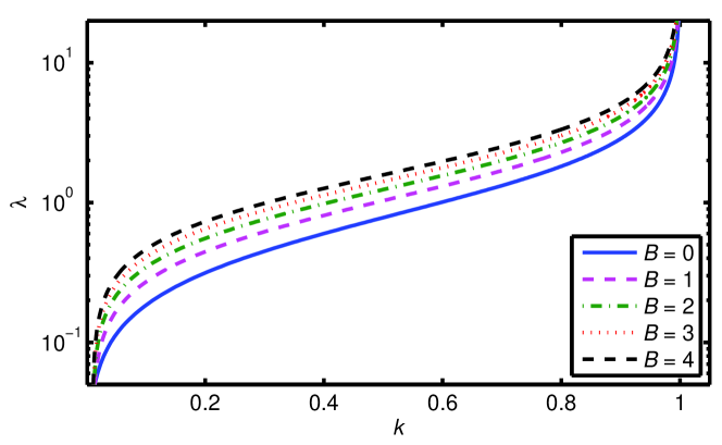
Figure 1: Growth coefficient $\lambda$ as a function of supersaturation $k$ at various levels of dislocation force amplitude $B$ for a circular plate ($d=2$) and $u_{s}=0.01u_{p}$.

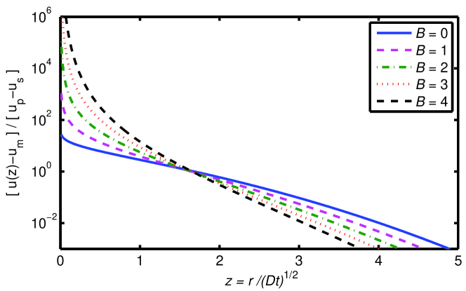
Figure 2: Reduced concentration field as a function of reduced distance from the surface of the circular plate ($d=2$) at various levels of dislocation force amplitude $B$ and at $\lambda=1$.

For $d=3$, i.e., a spherical second-phase particle in the absence of dislocation field ($B=0$), we find

$$u(z) = u_{m}+2q_{u}\lambda^{3}e^{\lambda^{2}}\Big{[}\frac{2e^{-z^{2}/4}}{z}-\sqrt{\pi}\,\mathrm{erfc}(z/2)\Big{]},$$ (18)

$$k = 2\lambda^{2}\Big{[}1-\sqrt{\pi}\,\lambda\,e^{\lambda^{2}}\mathrm{erfc}(\lambda)\Big{]}.$$ (19)

This corresponds to the results obtained by Frank Frank (1950).

For $d=3$ and $B=2$, equation (5) is simplified and an analytical solution can be found, resulting in

$$u(z) = \Bigg{(}\frac{e^{z^{2}/4}(z^{2}+2)\Big{[}\sqrt{\pi}\lambda e^{\lambda^{2}}\Big{(}\mathrm{erf}(\frac{z}{2})-\mathrm{erf}(\lambda)\Big{)}-1\Big{]}+2\lambda e^{\lambda^{2}}z}{\sqrt{\pi}\lambda e^{\lambda^{2}}\mathrm{erfc}(\lambda)-1}\Bigg{)}\frac{e^{-z^{2}/4}}{z^{2}}u_{m}+$$ (20)

$$+\;\Bigg{(}\frac{\lambda^{3}e^{\lambda^{2}}\Big{[}2z-\sqrt{\pi}e^{z^{2}/4}(z^{2}+2)\mathrm{erfc}(\frac{z}{2})\Big{]}}{\sqrt{\pi}\lambda e^{\lambda^{2}}\mathrm{erfc}(\lambda)-1}\Bigg{)}\frac{e^{-z^{2}/4}}{z^{2}}q_{u}.$$

Putting $u(2\lambda)=u_{s}$, we obtain

$$k=\frac{1+2\lambda^{2}\Big{(}1-\sqrt{\pi}\lambda\,e^{\lambda^{2}}\mathrm{erfc}(\lambda)\Big{)}}{2\lambda^{2}\Big{(}\sqrt{\pi}\lambda\,e^{\lambda^{2}}\mathrm{erfc}(\lambda)-1\Big{)}}\;\frac{u_{m}}{q_{u}}+\frac{2\lambda^{2}-(1+2\lambda^{2})\sqrt{\pi}\lambda\,e^{\lambda^{2}}\mathrm{erfc}(\lambda)}{2\Big{(}\sqrt{\pi}\lambda\,e^{\lambda^{2}}\mathrm{erfc}(\lambda)-1\Big{)}}.$$ (21)

For $u_{s}<<u_{p}$, we write

$$k=-2\lambda^{4}+\sqrt{\pi}\lambda^{3}(1+2\lambda^{2})\,e^{\lambda^{2}}\mathrm{erfc}(\lambda)+\Big{(}1-2\lambda^{2}+2\sqrt{\pi}\lambda^{3}\,e^{\lambda^{2}}\mathrm{erfc}(\lambda)\Big{)}\epsilon+\mathcal{O}(\epsilon^{2}).$$ (22)

General analytical expressions of $u(z)$ and $k$, in terms of confluent hypergeometric functions, can also be found for even values of $B$ as detailed in appendix A. Furthermore, asymptotic forms of $u(z)$ for large and small $z$ can be calculated, see appendix A for analysis of $z>>1$. Figure 3 compares $k$ versus $\lambda$ for $d=2$ and $d=3$ in the absence of dislocation field ($B=0$).

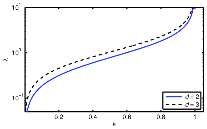
Figure 3: Growth coefficient $\lambda$ as a function of supersaturation parameter $k$ at $B=0$ for a circular plate ($d=2$) versus a sphere ($d=3$).

IV Discussion

The potential energy in equation (3) describes the elastic energy of the dislocation relaxed within the volume occupied by the second-phase precipitate Cahn (1957). It was treated here as an external field affecting the diffusion-limited growth of second-phase precipitate. The interaction energy of impurities in a crystalline with dislocations depends on the specific model or configuration of a solute atom and a matrix which is used. Commonly, it is assumed that the solute acts as an elastic center of dilatation. It is a fictitious sphere of radius $R^{\prime}$ embedded concentrically in a spherical hole of radius $R$ cut in the matrix. If the elastic constants of the solute and matrix are the same, the work done in inserting the atom in the presence of dislocation is $w=p\Delta v$, where $p$ is the hydrostatic pressure and $\Delta v$ is the difference between the volume of the hole in the matrix and the sphere of the fictitious impurity. For a screw dislocation $p=0$, while near an edge dislocation $p=\frac{(1+\nu)bG\sin\theta}{3\pi(1-\nu)r}$ for an impurity with polar coordinates $(r,\theta)$ with respect to the dislocation $0z$, hence $w\propto\Delta v\sin\theta/r$ Cottrell and Bilby (1949). Using a nonlinear elastic theory Nabarro (1987), a screw dislocation may also interact with the spherical impurity with the interaction energy $w\propto\Delta v/r^{2}$. Moreover, accounting for the differences in the elastic constants of a solute and a matrix, the solute will relieve shear strain energy as well as dilatation energy, which will also interact with a screw dislocation with a potential $w\propto\Delta v/r^{2}$ Friedel (1967). Indeed, Friedel Friedel (1967) has formulated that by introducing a dislocation into a solid solution of uniform concentration $c_{0}$, the interaction energy between the dislocation and solute atoms can be written as $w\backsimeq w_{0}(b/\delta)^{n}f(\theta)$, where $\delta$ is the distance between the two defects, $w_{0}$ the binding energy when $\delta=b$, and $f(\theta)$ accounts for the angular dependence of the interaction along the dislocation. Also, $n=1$ for size effects and $n=2$ for effects due to differences in elastic constants. The discussed model for the interaction energy between solute atoms and dislocations has been used to study the precipitation process on dislocations by number of workers in the past Ham (1959); Bullough and Newman (1962) and thoroughly reviewed in Bullough and Newman (1970). These studies concern primarily the overall phase transformation (precipitation of a new phase) rather than the growth of a new phase considered in our note. That is, they used different boundary conditions as compared to the ones used here.

Let us now link the supersaturation parameter $k$ to an experimental situation. For this purpose, the values of $u_{s}$, i.e. the concentration at the interface between the second-phase and matrix should be known. The capillary effect leads to a relationship between $u_{s}$ and the equilibrium composition $u_{eq}$ (solubility line in a phase diagram). To obtain this relationship, we consider an incoherent nucleation of second-phase on a dislocation à la Cahn Cahn (1957). A Burgers loop around the dislocation in the matrix material around the incoherent second-phase (circular plate) will have a closure mismatch equal to $b$. Following Cahn, on forming the incoherent plate of radius $R$, the total free energy change per unit length is

$$\mathcal{G}=-\pi R^{2}\Delta g_{v}+2\pi\gamma R-A^{\prime}\ln(R/r_{0}),$$ (23)

where $\Delta g_{v}$ is the volume free energy of formation, $\gamma$ the interfacial energy and the last term is the dislocation energy, $A^{\prime}=Gb^{2}/4\pi$ for screw dislocations, cf. equation (3). Setting ${\rm d}\mathcal{G}/{\rm d}R=0$, yields

$$R=\frac{\gamma}{2\Delta g_{v}}\Big{(}1\pm\sqrt{1-\alpha}\Big{)},$$ (24)

where $\alpha=2A^{\prime}\Delta g_{v}/\pi\gamma^{2}$. So, if $\alpha>1$, the nucleation is barrierless, i.e., the phase transition kinetics is only governed by growth kinetics, which is the subject of our investigation here. If, however, $\alpha<1$, there is an energy barrier and the local minimum of $\mathcal{G}$ at $R=R_{0}$, which corresponds to the negative sign in equation (24), ensued by a maximum at $R=R^{\ast}$ corresponding to the positive sign in this equation. The local minimum corresponds to a subcritcal metastable particle of the second-phase surrounding the dislocation line, and it is similar to the Cottrell atmosphere of solute atoms in a segregation problem. When $\alpha=0$, corresponding to $B=0$, the two phases are in equilibrium and the maximum in $\mathcal{G}$ is infinite, as for homogeneous nucleation.

For a dilute regular solution, $\Delta g_{v}=(k_{B}T/V_{p})\ln(u_{s}/u_{eq})$, where $V_{p}$ is the atomic volume of the precipitate compound, $u_{s}$ is the concentration of the matrix at a curved particle/matrix interface and $u_{eq}$ that of a flat interface, which is in equilibrium with the solute concentration in the matrix. Equation (24) gives $\Delta g_{v}=\gamma/R-A^{\prime}/2\pi R^{2}$. Hence, for a dilute regular solution, we write

$$u_{s}=u_{eq}\exp{\Big{[}\frac{\zeta}{R}\Big{(}1-\frac{\eta}{R}\Big{)}\Big{]}},$$ (25)

where $\zeta=\beta V_{p}\gamma$, $\beta=1/k_{B}T$ and $\eta=A^{\prime}/2\pi\gamma$. Subsequently, the supersaturation parameter is expressed by

$$k=\frac{u_{eq}\exp[{\frac{\zeta}{R}(1-\frac{\eta}{R})}]-u_{m}}{u_{p}-u_{eq}\exp[\frac{\zeta}{R}(1-\frac{\eta}{R})]}.$$ (26)

Taking the following typical values: $\gamma=0.2$ Jm^-2, $G=40$ GPa, and $b=0.25$ nm, then $A^{\prime}\approx 2.0\times 10^{-10}$ N and $\eta=0.16$ nm. Figure 4 depicts $u_{s}/u_{eq}$, from equation (25), as a function of scaled radius $R/\zeta$ for $V_{p}=1.66\times 10^{-29}$ m³, $\eta=0$ and $\eta=0.16$ nm at $T=600$ K. Equation (25) is analogous to the Gibbs-Thomson-Freundlich relationship Christian (2002) comprising a dislocation defect.

Recalling now the values used for the interaction parameter $B$ in the computations presented in the foregoing section, we note that for $B=2$ and the above numerical values for $G$ and $b$ at $T=1000$ K, we find $l\approx 0.14$ nm, which is close to the calculated value of $\eta$.

In Cahn’s model, the assumption that all the strain energy of the dislocation within the volume occupied by the nucleus can be relaxed to zero demands that the nucleus is incoherent. For a coherent nucleus forming on or in proximity of dislocations, this supposition is not true. Instead, it is necessary to calculate the elastic interaction energy between the nucleus and the matrix, which for an edge dislocation is in the form $Gb^{2}/[4\pi(1-\nu)r]$ for the energy density per unit length Barnett (1971). In the same manner, to extend our calculations for growth of coherent precipitate, we must employ this kind of potential energy, i.e. the potential energy of the form $\phi(r)=-A\ln(r/r_{0})+C\sin\theta/r$, in the governing kinetic equation rather than relation (3).

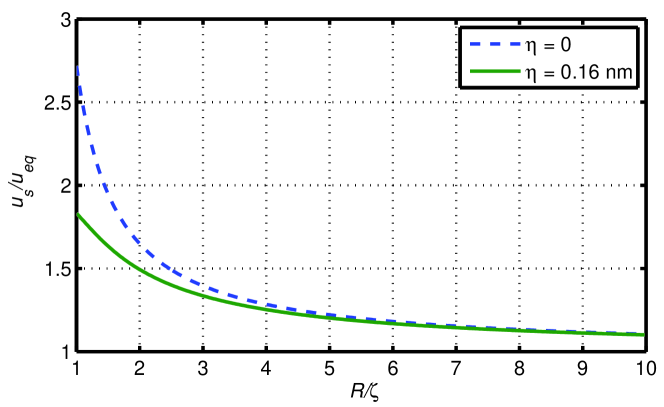
Figure 4: The size dependence of the concentration at the curved precipitate/matrix interface $u_{s}$ relative to that of the flat interface $u_{eq}$ for a set of parameter values given in the text, cf. eq. (25).

Appendix A Evaluation of solutions of equation (5) for $d=3$

For an ordinary second-order differential equation with a regular singularity, the Frobenius method can be used to obtain power series solution. On the other hand, when singularity is irregular, no convergent solution may be found; nevertheless, albeit divergent, the solution can be asymptotic. Let us write equation (5) for $d=3$ in a generic form

$$u^{\prime\prime}+p(z)u^{\prime}+q(z)u=0,$$ (27)

where primes denote differentiation with respect to $z$, $p(z)=z/2+(2+B)/z$ and $q(z)=B/z^{2}$. Since we have imposed the boundary condition $u(\infty)=u_{m}$, it is worthwhile to explore the behavior of the solution as $z\to\infty$. But, first let us put equation (27) in a more convenient form by setting $u(z)=\widetilde{u}(z)\exp[-\frac{1}{2}\int p(z)dz]$, which gives $\widetilde{u}^{\prime\prime}+(q-p^{\prime}/2+p^{4})\widetilde{u}=0$. Here, without loss of generality, we consider

$$u^{\prime\prime}+f(z)u = 0,$$ (28)

$$\text{where}\qquad f(z) = -\frac{z^{2}}{16}-\frac{B+3}{4}-\frac{B(B-2)}{4z^{2}}.$$ (29)

Since $f(z)$ is not $\mathcal{O}(z^{-2})$ as $z\to\infty$, then the point at infinity is an irregular singularity for $u(z)$. We now look for solutions of (28) by considering

$$u(z)\sim\exp\Big{(}\sum_{n=0}^{\infty}\psi_{n}(z)\Big{)},$$ (30)

where $\{\psi_{n}(z)\},n=0,1,\dots$, is an asymptotic sequence as $z\to\infty$. Substituting (30) into equation (28)

$$\psi_{0}^{\prime\prime}+\psi_{1}^{\prime\prime}+\dots+(\psi_{0}^{\prime}+\psi_{1}^{\prime}+\dots)^{2}+f(z)\sim 0,$$ (31)

where we have tacitly assumed that $\psi_{n}(z)$ is (twice) differentiable and the resulting series are still asymptotic.

Equation (31) is used to determine the $\{\psi_{n}(z)\},n=0,1,\dots$ by successively applying the asymptotic limit $z\to\infty$. The results for the first few terms are shown in table 1. Hence, we write for $z\to\infty$:

$$u_{+}(z) \sim A_{1}e^{z^{2}/8}z^{(1+B/2)}\Big{[}1+\frac{B}{z^{2}}+\mathcal{O}(z^{-4})\Big{]},$$ (32)

$$u_{-}(z) \sim A_{2}e^{-z^{2}/8}z^{-(B/2+2)}\Big{[}1-\frac{3(B+2)}{z^{2}}+\mathcal{O}(z^{-4})\Big{]},$$ (33)

where $A_{1}$ and $A_{2}$ are arbitrary constants. Note that the solution (32) is divergent for large $z$, whereas (33) is convergent and thus is physically admissible. Considering $u(\infty)=u_{m}$, we write

$$u_{-}(z)\sim u_{m}+A_{2}e^{-z^{2}/8}z^{-B/2-2}\Big{[}1-\frac{3(B+2)}{z^{2}}+\mathcal{O}(z^{-4})\Big{]},\;\text{as}\;z\to\infty.$$ (34)

Table 1: Solutions to equation (31).

Sequence	Solution 1	Solution 2
$\psi_{0}$	$z^{2}/8$	$-z^{2}/8$
$\psi_{1}$	0	0
$\psi_{2}$	$(\frac{B+2}{2})\ln z$	$-(\frac{B+4}{2})\ln z$
$\psi_{3}$	0	0
$\psi_{4}$	$Bz^{-2}$	$-3(B+2)z^{-2}$

Let us now evaluate the general solution to equation (5) for $d=3$ as expressed by equation (9). We apply the flux conservation relation (6) to obtain $C_{1}$, and then substitute $C_{1}$ in equation (9) to write

$$u(z)=K_{1}(z,B)C_{2}+K_{2}(z,B)q,$$ (35)

where

$$K_{1}(z,B) = \Big{(}\frac{2}{z}\Big{)}^{B}{{}_{1}\!F}_{1}\Big{(}-\frac{B}{2};\frac{3-B}{2};-\frac{z^{2}}{4}\Big{)}+$$ (36)

$$+\frac{B\lambda^{-B}{{}_{1}\!F}_{1}\Big{(}\frac{2-B}{2};\frac{5-B}{2};-\lambda^{2}\Big{)}}{B-3}K_{2}(z,B),$$

$$K_{2}(z,B) = \frac{4(B+1)\lambda^{3}{{}_{1}\!F}_{1}(-\frac{1}{2};\frac{1+B}{2};-\frac{z^{2}}{4})/z}{(B^{2}-1){{}_{1}\!F}_{1}(-\frac{1}{2};\frac{1+B}{2};-\lambda^{2})+2\lambda^{2}{{}_{1}\!F}_{1}(\frac{1}{2};\frac{3+B}{2};-\lambda^{2})},$$ (37)

$$K_{2}(z,0) = 2\lambda^{3}e^{\lambda^{2}}\Big{[}\frac{2e^{-z^{2}/4}}{z}+\sqrt{\pi}\,\mathrm{erf}(z/2)\Big{]}.$$ (38)

Here, ${{}_{1}\!F}_{1}(a;b;z)$ is the confluent hypergeometric function. If $a<0$, and either $b>0$ or $b<a$, this function can be expressed as a polynomial with finite number of terms. If, however, $b=0$ or a negative integer, then ${{}_{1}\!F}_{1}(a;b;z)$ itself is infinite. Thus, relations (37)-(38) become singular for $B=1,3,5,7,\dots$, making the solutions meaningless. Some useful relations for computations are listed in table 2. Additional relations and properties for ${{}_{1}\!F}_{1}(a;b;z)$ can be found in Abramowitz and Stegun (1964).

Next, we utilize the remote boundary condition $u(\infty)=u_{m}$ to determine $C_{2}$, then we formally write

$$u(z)=\frac{K_{1}(z,B)}{K_{1}(\infty,B)}u_{m}+\Big{(}K_{2}(z,B)-\frac{K_{1}(z,B)}{K_{1}(\infty,B)}K_{2}(\infty,B)\Big{)}q.$$ (39)

In computations of $K_{1}(\infty,B)$ prudence must be exercised, i.e., first evaluate this quantity for a given value of $B$, then take the limit $z\to\infty$. Note also that $K_{1}(z,0)=1$ $\forall z$ and $K_{2}(\infty,0)=2\sqrt{\pi}\lambda^{3}e^{\lambda^{2}}$.

Furthermore, we may calculate a relation for the supersaturation parameter, $k=(u_{s}-u_{m})/(u_{p}-u_{s})$, defined in the main text by using the condition $u(2\lambda)=u_{s}$ on equation (35), which gives

$$k=\Bigg{(}\frac{K_{1}(2\lambda,B)}{K_{1}(\infty,B)}-1\Bigg{)}\frac{u_{m}}{q}+K_{2}(2\lambda,B)-\frac{K_{1}(2\lambda,B)}{K_{1}(\infty,B)}K_{2}(\infty,B).$$ (40)

For dilute alloys, $u_{s}<<u_{p}$; so with $\epsilon\equiv u_{s}/u_{p}$, we write

$$k=\Bigg{(}1-\frac{K_{1}(\infty,B)}{K_{1}(2\lambda,B)}\Bigg{)}\epsilon+\frac{K_{2}(2\lambda,B)}{K_{1}(2\lambda,B)}K_{1}(\infty,B)-K_{2}(\infty,B)+\mathcal{O}(\epsilon^{2}).$$ (41)

Table 2: Special cases of ${{}_{1}\!F}_{1}(a;b;z)$.

${{}_{1}\!F}_{1}(-1;\frac{1}{2};-z^{2})=1+2z^{2}$

${{}_{1}\!F}_{1}(-\frac{1}{2};\frac{1}{2};-z^{2})=e^{-z^{2}}+\sqrt{\pi}z\,\mathrm{erf}(z)$

${{}_{1}\!F}_{1}(-\frac{1}{2};\frac{3}{2};-z^{2})=\frac{1}{2}e^{-z^{2}}+\frac{\sqrt{\pi}}{4}(1+2z^{2})\mathrm{erf}(z)z^{-1}$

${{}_{1}\!F}_{1}(\frac{1}{2};\frac{3}{2};-z^{2})=\frac{\sqrt{\pi}}{2}\mathrm{erf}(z)z^{-1}$

${{}_{1}\!F}_{1}(\frac{1}{2};\frac{5}{2};-z^{2})=\frac{3}{8}\Big{(}2ze^{-z^{2}}+\sqrt{\pi}(2z^{2}-1)\mathrm{erf}(z)\Big{)}z^{-3}$

References

- Larché (1979) F. C. Larché, in Dislocations in Solids, edited by F. R. N. Nabarro (North-Holland Publishing Company, Amsterdam, Holland, 1979), vol. 4.
- Wagner and Kampmann (1991) R. Wagner and R. Kampmann, in Phase Transformation in Materials, edited by E. K. R.W. Cahn, P. Haasen (VCH, Weinheim, Germany, 1991), vol. 5 of Materials Science and Technology, chap. 4, volume editor P. Haasen.
- Porter and Easterling (1981) D. Porter and K. Easterling, Phase Transformations in Metals and Alloys (Chapman Hall, London, UK, 1981), chap 5.
- Christian (2002) J. W. Christian, The Theory of Transformations in Metals and Alloys (Pergamon, Amsterdam, 2002), part I.
- Aaronson et al. (1971) H. I. Aaronson, H. Aaron, and L. Kinsman, Metallography 4, 1 (1971).
- Aaron and Aaronson (1971) H. Aaron and H. I. Aaronson, Metallurgical Transactions 2, 23 (1971).
- Allen and Vander Sande (1978) R. M. Allen and J. B. Vander Sande, Metallurgical Transactions A 9A, 1251 (1978).
- Deschamps et al. (1999) A. Deschamps, F. Livet, and Y. Brechet, Acta Materialia 47, 281 (1999).
- Deschamps and Brechet (1999) A. Deschamps and Y. Brechet, Acta Materialia 47, 293 (1999).
- Cahn (1957) J. W. Cahn, Acta Metallurgica 5, 169 (1957).
- Blavette et al. (1999) D. Blavette, E. Cadel, A. Fraczkiewicz, and A. Menand, Science 286, 2317 (1999).
- Thompson et al. (2007) K. Thompson, P. L. Flaitz, P. Ronsheim, D. J. Larson, and T. F. Kelly, Science 317, 1370 (2007).
- Cottrell and Bilby (1949) A. H. Cottrell and B. A. Bilby, Proc. Phys. Soc. A 62, 49 (1949).
- Harper (1951) S. Harper, Physical Review 83, 709 (1951).
- Bullough and Newman (1970) R. Bullough and R. C. Newman, Reports in Progress of Physics 33, 101 (1970).
- Frank (1950) F. C. Frank, Proc. Roy. Soc. London A 201, 586 (1950).
- Carslaw and Jaeger (1959) H. S. Carslaw and J. C. Jaeger, Conduction of Heat in Solids (1959), 2nd ed.
- Aaron et al. (1970) H. B. Aaron, D. Fainstein, and G. R. Kotler, J. Appl. Phys. 41, 4404 (1970).
- Köster et al. (1996) U. Köster, J. Meinhardt, S. Roos, and H. Liebertz, Appl. Phys. Lett. 69, 179 (1996).
- Massih et al. (2003) A. R. Massih, T. Andersson, P. Witt, M. Dahlbäck, and M. Limbäck, J. Nucl. Mater. 322, 138 (2003).
- Sundar and Hoyt (1992) G. Sundar and J. J. Hoyt, Journal of Physics: Condensed Matter 4, 4359 (1992).
- Chandrasekhar (1943) S. Chandrasekhar, Reviews of Modern Physics 15, 1 (1943).
- Kittel (1996) C. Kittel, Introduction to Solid State Physics (John Wiley & Sons, New York, 1996), 7th ed.
- Friedel (1967) J. Friedel, Dislocations (Pergamon Press, Oxford, UK, 1967).
- Abramowitz and Stegun (1964) M. Abramowitz and I. A. Stegun, Handbook of Mathematical Functions (Dover Publications, New York, 1964).
- Nabarro (1987) F. R. N. Nabarro, Theory of Crystal Dislocations (Dover Publications, 1987).
- Ham (1959) F. S. Ham, J. Appl. Phys. 6, 915 (1959).
- Bullough and Newman (1962) R. Bullough and R. C. Newman, Proc. Roy. Soc. A 266, 198 (1962).
- Barnett (1971) D. M. Barnett, Scripta Metallurgica 5, 261 (1971).