On blow-up shock waves for a nonlinear
PDE associated with Euler equations

Abstract.

The following nonlinear PDE:

$$\textstyle{\big{(}\frac{u_{t}}{u}\big{)}_{t}=\frac{u_{x}u_{t}}{u}\quad\mbox{in\,\, $\mathbb{R}\times\mathbb{R}_{+}$},}$$

derived from 2D Euler equations, is shown to admit smooth similarity solutions, which as $t\to T^{-}$ create shocks of the type ${\rm sign}\,x$ and $H(-x)$ and also other blow-up singularities. Some of the blow-up solutions are shown to admit unique extension beyond, for $t>T$. All the similarity reductions lead to singular boundary value problems for 2nd-order ODEs. More complicated solutions with blow-up angular swirl are discussed.

1. Introduction: Euler equations and a related PDE with shock waves

1.1. Euler equations and shocks: beginning of derivation

Consider the 2D Euler equations (the EEs) of inviscid incompressible fluids

(1.1) $${\bf u}_{t}+({\bf u}\cdot\nabla){\bf u}=-\nabla p,\quad{\rm div}\,{\bf u}=0\quad\mbox{in}\quad\mathbb{R}^{2}\times(0,T)\quad({\bf u}=(u_{1},u_{2})^{T}),$$

with bounded initial divergence-free ${\bf u}_{0}$ of infinite kinetic $L^{2}$-energy. Using Leray’s formulation with the projector ${\mathbb{P}}=I-\nabla\Delta^{-1}(\nabla\cdot)$, (1.1) is written in the form [12, p. 30]

(1.2) $$\begin{matrix}{\bf u}_{t}+(D{\bf u})\,{\bf u}={\bf B}({\bf u})\equiv\frac{1}{2\pi}\,\int\limits_{\mathbb{R}^{2}}\frac{{\bf x}-{\bf y}}{|{\bf x}-{\bf y}|^{2}}\,{\rm tr}\,(\nabla{\bf u}({\bf y},t))^{2}\,{\mathrm{d}}{\bf y},\quad\mbox{where}\quad\\ {\rm tr}\,(\nabla{\bf u})^{2}=\sum\limits_{(i,j)}(u_{j})_{x_{i}}(u_{i})_{x_{j}}\quad\mbox{and}\quad D{\bf u}=\left[\begin{matrix}(u_{1})_{x_{1}}\,\,\,(u_{1})_{x_{2}}\vskip 3.0pt plus 1.0pt minus 1.0pt\\ (u_{2})_{x_{1}}\,\,\,(u_{2})_{x_{2}}\end{matrix}\right]\end{matrix}$$

is the $2\times 2$ Jacobian matrix of the solenoidal vector field ${\bf u}$.

It is well-known that, even in dimension 2 (to say nothing about the 3D ones), the standard notion of weak solutions is not sufficient for establishing the unique solvability of the problem in the case of the unbounded initial vorticity, where ${\rm curl}\,{\bf u}_{0}\not\in L^{\infty}$. See Majda–Bertozzi [12, § 8] and recent surveys in Bardos–Titi [1], Constantin [4], and Ohkitani [13] for further details and key references, as well as Pomeau et al [17] for discussion of somehow related open questions on shock waves in hyperbolic systems. It seems obvious that natural reasons for this difficulty are two fold. Firstly, there is no still a proper definition of “entropy solutions” for the EEs admitting sufficiently strong “shock waves”. In other words, general principles of formation of various singularities of shock wave types, as well as $L^{\infty}$-blow-up, are in general unknown. Secondly, on the other hand, even the corresponding system without the nonlocal term

(1.3) $${\bf u}_{t}+(D{\bf u}){\bf u}=0\quad\mbox{in}\quad\mathbb{R}^{2}\times\mathbb{R}_{+}$$

is a rather difficult divergent hyperbolic system $2\times 2$ with two independent spatial variables ${\bf x}=(x_{1},x_{2})$, so it does not automatically fall into the scope of modern entropy theory regardless of its definite recent achievements; see Bressan [2] and Dafermos [5]. Of course, some classes of solutions of systems such as (1.3) can be represented via characteristics (see interesting physically motivated formal discussions in [17]), though, in general, choosing right weak “entropy” solutions is not straightforward and is an open problem.

Our goal is to introduce a new PDE model, which may reflect some features of formation of finite-time singularities in systems such as (1.1) (and partially (1.3)) and, in addition, having vorticity-swirl structure that can be somehow adequate to the EEs. To this end, to discuss possible ways of shock wave formation for the EEs, let us write down (1.1) in the polar coordinates $(r,\varphi)$,

(1.4) $$\left\{\begin{matrix}U_{t}+UU_{r}+\frac{1}{r}\,VU_{\varphi}-\frac{1}{r}\,V^{2}=-P_{r},\quad\vskip 3.0pt plus 1.0pt minus 1.0pt\\ V_{t}+UV_{r}+\frac{1}{r}\,VV_{\varphi}+\frac{1}{r}\,UV=-\frac{1}{r}\,P_{\varphi},\vskip 3.0pt plus 1.0pt minus 1.0pt\\ U_{r}+\frac{1}{r}\,U+\frac{1}{r}\,V_{\varphi}=0.\qquad\qquad\qquad\,\,\,\end{matrix}\right.$$

Though (1.4) is a system of three PDEs, which is equivalent to the nonlocal equation (1.2), we consider a rather hypothetical situation of formation of shocks created by local differential operators only, though, as we have seen, this scenario is expected to be also relevant to the hyperbolic system (1.3).

Let us then more precisely define a manifold of solutions with shocks to be studied:

(i) Formation of bounded shocks (or bounded rarefaction waves) is not essentially affected by the pressure terms, i.e., by the nonlocal members (however, the div-free equation remains important); and

(ii) As in the classic case (1.7) below, two quadratic first-order operators in the first and in the second equations in (1.4) are leading together with two differential terms in the div-free equation (the latter is reasonable for finite shocks):

(1.5) $$\left\{\begin{matrix}U_{t}+UU_{r}+...=0,\,\,\,\vskip 3.0pt plus 1.0pt minus 1.0pt\\ V_{t}+\frac{1}{r}\,VV_{\varphi}+...=0,\vskip 3.0pt plus 1.0pt minus 1.0pt\\ U_{r}+\frac{1}{r}\,V_{\varphi}+...=0.\,\,\,\end{matrix}\right.$$

Thus, we omit other operators that are expected to be bounded on such singularities.

Replacing $V$ by $rV$ for convenience yields

(1.6) $$V\mapsto rV\quad\Longrightarrow\quad\left\{\begin{matrix}U_{t}+UU_{r}+...=0,\,\,\,\vskip 3.0pt plus 1.0pt minus 1.0pt\\ V_{t}+VV_{\varphi}+...=0,\,\,\vskip 3.0pt plus 1.0pt minus 1.0pt\\ U_{r}+V_{\varphi}+...=0.\,\,\,\,\,\end{matrix}\right.$$

The first two equations are indeed the famous 1D Euler equations from gas dynamics,

(1.7) $$u_{t}+uu_{x}=0\quad\mbox{in}\quad\mathbb{R}\times\mathbb{R}_{+},\quad u(x,0)=u_{0}(x)\in L^{1}\cap L^{\infty},$$

whose entropy theory was created by Oleinik [14, 15] and Kruzhkov [11] (equations in $\mathbb{R}^{N}$) in the 1950–60s; see details on the history, main results, and modern developments in the well-known monographs [2, 5, 20]. Typical formation of shocks for (1.7) as $t\to 0^{-}$ (the blow-up time here is $T=0$) is described by the canonical self-similar blow-up solution

(1.8) $$u_{-}(x,t)=\left\{\begin{matrix}1\quad\mbox{for}\quad x<t,\\ \,\,\,\,\frac{x}{t}\quad\mbox{for}\quad|\frac{x}{t}|<1,\\ -1\quad\mbox{for}\quad x>-t.\end{matrix}\right.$$

Therefore, the following steady shock is formed:

(1.9) $$\textstyle{\lim_{t\to 0^{-}}\,u_{-}(x,t)=S_{-}(x)\equiv-{\rm sign}\,x,}$$

with convergence in $L^{1}(\mathbb{R})$ and uniformly on any subset bounded away from the origin. Moreover, we have that, as $t\to 0^{-}$,

(1.10) $$\textstyle{D_{x}u_{-}(x,t)=\frac{1}{t}\to-\infty\,\,\,\mbox{for any}\,\,\,|x|<|t|\quad\mbox{and}\quad D_{x}u_{-}(x,t)\to-2\delta(x).}$$

Indeed, such a standard scenario of shock wave formation is not applicable for the system in (1.6), since the last div-free equation

(1.11) $$U_{r}+V_{\varphi}+...=0$$

prohibits simultaneous blow-up of derivatives $U_{r}$ and $V_{\varphi}$ to $-\infty$. Therefore, the system (1.6) needs another more involved treatment of possible (if any) shock waves. We next introduce such a nonlinear PDE model.

1.2. A simplified PDE model and main results

Thus, we consider first two equations in (1.6) on the “critical manifold” (1.11), i.e.,

(1.12) $$\left\{\begin{matrix}U_{t}+UU_{r}=0,\vskip 3.0pt plus 1.0pt minus 1.0pt\\ V_{t}+VV_{\varphi}=0\,\end{matrix}\right.\Big{|}_{U_{r}+V_{\varphi}=0}\quad\Longrightarrow\quad\framebox{$\left\{\begin{matrix}U_{t}=UV_{\varphi},\vskip 3.0pt plus 1.0pt minus 1.0pt\\ V_{t}=VU_{r},\end{matrix}\right.$}$$

with given bounded smooth initial data $(U_{0},V_{0})(r,\varphi)$. Writing this in the form

(1.13) $$\left\{\begin{matrix}(\ln|U|)_{t}=V_{\varphi},\vskip 3.0pt plus 1.0pt minus 1.0pt\\ (\ln|V|)_{t}=U_{r},\,\end{matrix}\right.$$

we find on integration of the second equation that

(1.14) $$\textstyle{\ln\big{|}\frac{V(t)}{V_{0}}\big{|}=\int_{0}^{t}U_{r}(s)\quad\Longrightarrow\quad V(t)=V_{0}{\mathrm{e}}^{\int_{0}^{t}U_{r}(s)}.}$$

Substituting this $V(t)$ into the first equation for $U$ yields the following nonlocal PDE:

(1.15) $$\textstyle{U_{t}=UV_{0\varphi}{\mathrm{e}}^{\int_{0}^{t}U_{r}(s)}+UV_{0}\,\big{(}{\mathrm{e}}^{\int_{0}^{t}U_{r}(s)}\big{)}\,{\int_{0}^{t}U_{r\varphi}(s)}\equiv J_{1}+J_{2}.}$$

According to (1.15), there exist at least two different mechanisms of shock wave formation corresponding to nonlinear integral operators $J_{1}$ and $J_{2}$, and possibly, other types via their nonlinear interactions. Note that the problem corresponding to $J_{2}$ is assumed to be truly 2D (and hence difficult), while that for $J_{1}$ can be reduced to 1D.

We begin with the simplest scenario corresponding to $J_{1}$, for which we choose initial data $V_{0}$ such that, in a small neighbourhood of a possible shock at $(0,0)$,

(1.16) $$V_{0\varphi}\approx+1\quad\mbox{and}\quad V_{0}\approx 0.$$

This locally yields the equation

(1.17) $$\textstyle{U_{t}=U{\mathrm{e}}^{\int_{0}^{t}U_{r}(s)}\quad\mbox{or}\quad\ln\big{(}\frac{U_{t}}{U}\big{)}={\int_{0}^{t}U_{r}(s)},\quad\mbox{where we assume}\,\,\,\frac{U_{t}}{U}>0.}$$

Differentiating this equation in $t$ and, for convenience, renaming the variables

(1.18) $$r\mapsto x\quad\mbox{and}\quad U(r,t)\mapsto u(x,t)$$

yields the necessary equation for such shock wave and blowing up formation:

(1.19) $$\textstyle{\big{(}\frac{u_{t}}{u}\big{)}_{t}=\frac{u_{x}\,u_{t}}{u}\quad\mbox{or}\quad\framebox{$uu_{tt}-(u_{t})^{2}=uu_{x}u_{t}.$}}$$

Written in the form with the evolution time-variable $x$ and $t$ being the space variable,

(1.20) $$\textstyle{u_{x}=\frac{1}{u_{t}}\big{[}u_{tt}-\frac{(u_{t})^{2}}{u}\big{]},}$$

the equation becomes

(1.21) of parabolic type in the domain of time-monotonicity $$\{u_{t}>0\}$$

and parabolic backward in time otherwise. In what follows, we will need carefully control the parabolicity condition (1.21) in order to guarantee the well-posedness of our shock and blow-up phenomena. In the original independent variables $\{x,t\}$, which assume two initial conditions at $t=0$, (1.19) exhibits different evolution properties. Note that, in terms of $t$ as the time variable, this equation

(1.22) $$\textstyle{u_{tt}=\frac{uu_{x}u_{t}+(u_{t})^{2}}{u}}$$

is in the normal form in the non-singular set $\{u\not=0\}$, so it obeys there the Cauchy–Kovalevskaya Theorem [21, p. 387]. Hence, for analytic initial data $u(x,0)\not=0$ and $u_{t}(x,0)$, there exists a unique local in time analytic solution $u(x,t)$. On the other hand, any existing solution $u(x,t)$, which is analytic in $\{u\not=0\}$, has a unique local analytic continuation at any point, where $u\not=0$.

Let us make an important comment concerning the type of this new PDE. Written as a first-order system for $U=(u,v)^{T}$, with $v=u_{t}$, (1.19) takes the form

(1.23) $$\textstyle{U_{t}=A(U)U_{x}+F(U),\quad\mbox{where}\quad A(U)=\left[\begin{matrix}0\,\,\,0\\ v\,\,\,0\end{matrix}\right]\quad\mbox{and}\quad F(U)=\left[\begin{matrix}v\\ \frac{v^{2}}{u}\end{matrix}\right].}$$

It follows that the characteristic equation for the matrix $A(U)$ has the trivial form

(1.24) $${\rm det}\,(A(U)-\lambda I_{2})=0\quad\Longrightarrow\quad\lambda^{2}=0.$$

Therefore the eigenvalues always coincide, $\lambda_{\pm}=0$, so that

(1.25) $$\mbox{(\ref{HS10}) is not a strictly hyperbolic system},$$

and indeed it is uniformly degenerate. In view of (1.25), application of classic theory of hyperbolic systems (see [2, 5]), which recently got a fundamental progress, is not possible. In any case, it is worth recalling that formation of singularities for (1.23) or (1.19) and possible extensions of blow-up solutions beyond singularities remain the key (and absolutely unavoidable for any difficult nonlinear PDE model) question to be addressed in what follows.

Regardless such nice local regularity and analyticity properties of the PDE (1.19), our main goal is to show that (1.19) admits rather standard “quasi-stationary” self-similar shock waves (Section 2) and other blow-up singularities (Section 3). In Section 4, following the strategy in [9], we develop a local theory of formation of shock waves from continuous data and show that the PDE (1.19) admits a unique similarity continuation after blow-up. In other words, this implies that uniqueness is not lost locally at the singularity blow-up points, and this links (1.19) with the classic model (1.7). However, a proper definition of entropy solutions to create a global existence-uniqueness theory for (1.19) remains a difficult open problem (it is not clear if such one can be developed in principle).

1.3. On blow-up similarity solutions with swirl

Let us for a while return to the full boxed system in (1.12), which is a difficult object, so we truly and desperately need a simplified model. For instance, in general, (1.12) admits complicated singular solutions with blow-up angular swirl. For the NSEs and EEs, such a mechanism was proposed in [7], so we omit details, and prescribe those similarity solutions as follows: for fixed $\alpha\in(0,1)$ and $\sigma\in\mathbb{R}$,

(1.26) $$\begin{matrix}U(r,\varphi,t)=(-t)^{-\alpha}f(y,\mu),\quad V(r,\varphi,t)=(-t)^{-1}g(y,\mu),\vskip 3.0pt plus 1.0pt minus 1.0pt\vskip 3.0pt plus 1.0pt minus 1.0pt\\ y=\frac{r}{(-t)^{\beta}},\quad\beta=1-\alpha,\quad\mu=\varphi+\sigma\ln(-t),\qquad\qquad\quad\end{matrix}$$

where we introduce blow-up rotation in the angular direction being a logarithmic travelling wave. Substituting (1.26) into (1.12) yields the following first-order system:

(1.27) $$\left\{\begin{matrix}\alpha f+\beta f^{\prime}_{y}y-\sigma f^{\prime}_{\mu}=fg^{\prime}_{\mu},\vskip 3.0pt plus 1.0pt minus 1.0pt\\ g+\beta g^{\prime}_{y}y-\sigma g^{\prime}_{\mu}=gf^{\prime}_{y}.\,\,\,\end{matrix}\right.$$

This is a difficult system, which we do not intent to study it here, though indeed some its features will be detected for a reduced simpler PDE model in (1.19).

2. Shock waves by blow-up similarity solutions

2.1. Existence of self-similar shock formation

Similar to (1.8), we look for blow-up similarity solutions of (1.19) of the form

(2.1) $$\textstyle{u_{-}(x,t)=f(y),\quad y=\frac{x}{(-t)},\quad\mbox{where}\quad\big{(}\frac{f^{\prime}y}{y}\big{)}^{\prime}+\frac{f^{\prime}}{f}=\frac{(f^{\prime})^{2}}{f}.}$$

The ODE in (2.1) can be easily reduced to the following one:

(2.2) $$yff^{\prime\prime}=(f^{\prime})^{2}(y+f)-2ff^{\prime},\quad f(\pm\infty)=\pm 1,$$

which is degenerate at $y=0$ and at any zero $f=0$ of solutions. Note that, unlike (1.8), the conditions at infinity have been changed, so that (2.1) is supposed to deliver the opposite shock:

(2.3) $$\textstyle{\lim_{t\to 0^{-}}\,u_{-}(x,t)=S_{+}(x)\equiv{\rm sign}\,x.}$$

In view of the obvious symmetry of (2.2):

(2.4) $$\left\{\begin{matrix}y\mapsto-y,\\ f\mapsto-f\end{matrix}\right.$$

it suffices to solve the following problem:

(2.5) $$yff^{\prime\prime}=(f^{\prime})^{2}(y+f)-2ff^{\prime}\quad\mbox{for}\quad y>0;\quad f(0)=0,\,\,\,f(+\infty)=1.$$

Recall that according to (1.17) we have to check the sign of

(2.6) $$\textstyle{\frac{u_{t}}{u}\equiv(-t)^{-1}\frac{f^{\prime}y}{f}>0}$$

which is true if $f(y)>0$ and $f^{\prime}(y)>0$ for all $y>0$. Here, (2.5) is a pretty standard second-order ODE, so we state the final result:

Theorem 2.1.

The problem $\eqref{20}$ admits a unique $C^{2}([0,\infty))$ strictly monotone solution.

Proof. It consists of a few steps. (i) Scaling invariance. One can see that (2.5) admits a group of scalings: if $f_{1}(y)$ is a solution,

(2.7) $$\textstyle{\mbox{then}\quad f_{a}(y)=af_{1}\big{(}\frac{y}{a}\big{)}\quad\mbox{is a solution for any $a\not=0$}.}$$

(ii) Finite regularity at $y=0$. This can be seen by (still formal) expansion near the origin

(2.8) $$f(y)=y+\varepsilon(y),\quad\mbox{where}\quad\varepsilon(y)=o(y)\quad\mbox{as}\quad y\to 0.$$

Substituting (2.8) into the ODE (2.5) and “linearizing” yields the following Euler’s ODE:

(2.9) $$\textstyle{y^{2}\varepsilon^{\prime\prime}-2y\varepsilon^{\prime}+\varepsilon=0\quad\Longrightarrow\quad\varepsilon(y)=y^{m_{\pm}},\quad\mbox{where}\quad m_{\pm}=\frac{3\pm\sqrt{5}}{2}.}$$

Since we are looking for sufficiently smooth and at least classical solutions of the PDE (1.19), we have to choose the maximal exponent

(2.10) $$\textstyle{m=m_{+}=\frac{3+\sqrt{5}}{2}=2.61803...\in(2,3)\quad(m_{-}=0.38197...<1).}$$

The justification of the expansion (2.8), (2.9) is performed in a standard manner by reducing the ODE to the equivalent integral equations for $y=y(f)$ (this deletes the trivial solution $f\equiv 0$) and applying Banach’s Contraction Principle with a suitable weighted functional setting.

Thus, (2.5) admits a 1D bundle of solutions close to the origin:

(2.11) $$f(y)=y+Ay^{m}+o(y^{m})\quad\mbox{for}\quad y>0,$$

where $A\in\mathbb{R}$ is arbitrary. For $A=0$, we have the exact unbounded solution

(2.12) $$f_{0}(y)=y.$$

It follows from the symmetry (2.4) that the extension of the shock profiles for $y<0$ is:

(2.13) $$f(y)=y+A|y|^{m-1}y+o(|y|^{m})\quad\mbox{for}\quad y<0.$$

The parameter $A<0$ makes it possible to shoot the necessary constant $+1$ at infinity, which is rather standard and we omit details. ∎

Actually, some necessary properties of solutions of (2.5) can be easily checked numerically by using a standard MatLab solvers such as the ode45, and this diminishes the necessity of a deeper mathematical study. In Figure 1, we show the monotone dependence on $A<0$ and $A>0$ of solutions of (2.5) with the expansion (2.11). For $A>0$, the local solutions $f(y)$ blow-up in finite $y_{0}>0$ that is also easily proved. Note that for $A<0$, according to (1.21), the behaviour in $\{y>0\}$ of similarity solutions (2.1) are locally governed by a well-posed parabolic flow with a blow-up formation of a shock wave in finite time.

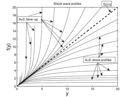
Figure 1. Various solutions of the ODE (2.5) with the expansion (2.11) for different values of $A>0$.

The next Figure 2 demonstrates a general view of similarity shock profiles for both $y>0$ and $y<0$. By the boldface line we denote the unique solution of the problem (2.5), with the following values in the expansion (2.11):

(2.14) $$A_{*}=-0.96...\,.$$

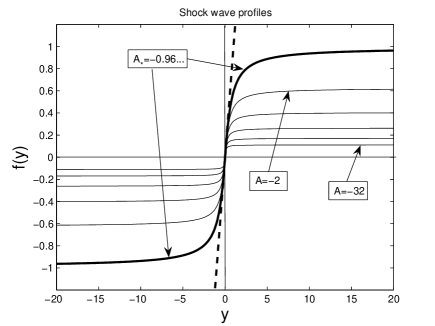
Figure 2. A general view of similarity shock profiles.

In addition, in Figure 3 we present the results of further analysis of shock wave profiles as (generalized) solutions of the ODE (2.5). Namely, we now shoot from $y=-50$ with the following asymptotic expansion of the solutions about the equilibrium $f=1$:

(2.15) $$\textstyle{f(y)=1+\frac{B}{y}+...\quad\mbox{as}\quad y\to-\infty.}$$

We now use the ode45 solver with the fully enhanced relative and absolute tolerances

(2.16) $$\mbox{Tols}=10^{-13}.$$

For $B<0$, we observe that the solutions pass though the singular point $y=0$ and converge to another larger equilibrium,

(2.17) $$f(y)\to f_{+}\quad\mbox{as}\quad y\to+\infty,\quad\mbox{where}\quad f_{+}=f_{+}(B)>1.$$

Note that possible singularities at $y=0$ are integrable since even in the worst case the solution is bounded,

$$\textstyle{f^{\prime\prime}\sim\frac{1}{y}\quad\Longrightarrow\quad f(y)\sim C+y\ln|y|+...\quad\mbox{as}\quad y\to 0,}$$

or the regularity is better, when the right-hand side in (2.5) vanishes at $y=0$ (this case actually occurs to give good solutions).

A different phenomenon is observed for $B>0$, where the shock profiles seem have finite interfaces at some $y=y_{0}<0$. However, next Figure 4 explains that this is wrong: thought (a) with the enlargement $10^{-3}$ continues to convince existence of negative finite interfaces, (b) given in the logarithmic scale confirms that the solutions have exponential decay up to $y=0^{-}$. Some lines in (b) are disjoint for profiles $|f(y)|\sim 10^{-17}$, which suddenly change sign due to numerical errors (recall the guaranteed accuracy (2.16)). Namely, a more careful look at the equation (2.5) shows that it admits solutions with the following typical non-analytic behaviour:

(2.18) $$\textstyle{f(y)\sim{\mathrm{e}}^{-\frac{a}{(-y)}}\to 0\quad\mbox{as}\quad y\to 0^{-},}$$

where $a>0$ is arbitrary due to the scaling symmetry (2.7).

Such solutions admit a natural trivial extension by $f(y)\equiv 0$ for $y\geq 0$, thus forming $C^{\infty}$ shock wave solutions with finite interfaces. Taking such a profile $f(y)$, instead of (1.9), we get in the limit the reflected Heaviside function:

(2.19) $$\lim_{t\to 0^{-}}u_{-}(x,t)=H(-x)=\left\{\begin{matrix}0\quad\mbox{for}\quad x\geq 0,\\ 1\quad\mbox{for}\quad x<0.\end{matrix}\right.$$

It is principal to note that, due to the regularity (2.18) at the interface, the similarity solution (2.1) is a $C^{\infty}$ function for $t<0$. In other words, (2.19) describes formation of a shock wave as $t\to 0^{-}$ from classic $C^{\infty}$ solutions. Such an evolution process of formation of shocks can be taken as a core property for introducing a test on the so-called $\delta$-entropy solutions, i.e., those which are obtained via smooth deformation of shocks appeared. See [6, 8, 10], where such an approach is developed for nonlinear dispersion equations such as

(2.20) $$u_{t}=(uu_{x})_{xx}\quad\mbox{and}\quad u_{t}=-(uu_{x})_{xxxx}.$$

Classic concepts of entropy do not apply to (2.20), so other approaches are needed. On the other hand, a detailed pointwise analysis of formation of gradient blow-up for PDEs such as (2.20) shows that uniqueness is violated there, so a consistent entropy theory is most plausibly non-existent in principle; see [9]. Deeper evolution and entropy-like properties of such finite interface solutions are out of the scope of this paper. Let us mention that the questions on weak compactly supported solutions are in the focus of modern research in the EEs area; see [1, p. 418].

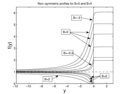
Figure 3. Examples of non-symmetric similarity shock profiles satisfying (2.15) for $B<0$ and $B>0$.

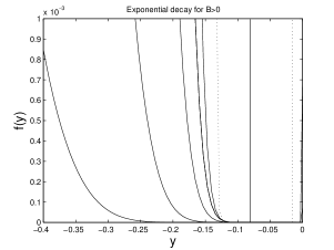
(a) Enlargement $10^{-3}$

(b) Logarithmic scale

Figure 4. Enlarged shock profiles for $B>0$: exponential decay as $y\to 0^{-}$.

2.2. Existence of rarefaction waves

The corresponding rarefaction waves describe collapse of initial singularities. The similarity ones then are defined for all $t>0$:

(2.21) $$\textstyle{u_{+}(x,t)=F(y),\quad y=\frac{x}{t},\quad yFF^{\prime\prime}=(F^{\prime})^{2}(y-F)-2FF^{\prime},\quad F(\pm\infty)=\mp 1.}$$

It follows that, in comparison with the shock profiles $F(y)$ constructed above, the rarefaction ones are given by the reflection:

(2.22) $$-F(y)\quad\mbox{is a solution of the rarefaction ODE (\ref{16R}).}$$

Therefore, the similarity solution in (2.21) is formed by the initial singularity $S_{-}(x)=-{\rm sign}\,x$ and describes its evolution collapse for $t>0$.

Similarly, for data $u(x,0)=-H(-x)$, we obtain similarity solution (2.21) describing its collapse. To get a unique solution, two initial functions should be prescribed. It is easy to see that $u_{t}(x,0)$ is not a distribution. Indeed, we have, according to (2.21) and asymptotics (2.15), (2.18), in the sense of distributions, it is formally valid that

(2.23) $$\textstyle{u_{t}(x,t)=-\frac{1}{t}\,F^{\prime}(y)y\to a_{0}\delta(x)\quad\mbox{as}\quad t\to 0^{+},\quad\mbox{where}\quad a_{0}=-\int F^{\prime}(y)y\,{\mathrm{d}}y>0.}$$

However, in view of the asymptotics (2.15), the integral in (2.23) diverges, so that $u_{t}(x,0)$ is not a bounded positive measure. In the sense of distributions, such a behaviour can be characterized by a logarithmic divergence as follows:

(2.24) $$\textstyle{u_{t}(x,t)=-\frac{1}{t}\,F^{\prime}(y)y\sim B|\ln t|\,\delta(x)\quad\mbox{as}\quad t\to 0^{+},\quad\mbox{so \,$\frac{u_{t}}{|\ln t|}(x,0)$\, is a measure}.}$$

3. Unbounded shocks by similarity blow-up and rarefaction profiles

More complicated shock-type structure occurs if in (2.1) we introduce a parameter $\alpha\in(0,1)$ looking for similarity solutions (cf. (1.26))

(3.1) $$\textstyle{u_{-}(x,t)=(-t)^{-\alpha}f(y),\quad y=\frac{x}{(-t)^{\beta}}\quad\mbox{for}\quad t<0,\quad\mbox{where}\quad\beta=1-\alpha,}$$

and $f(y)$ then solves the following more complicated ODE:

(3.2) $$\beta^{2}y^{2}ff^{\prime\prime}=\beta y(f^{\prime})^{2}(\beta y+f)+\beta(\alpha-2)yff^{\prime}+\alpha f^{2}(f^{\prime}-1)\quad\mbox{in}\quad\mathbb{R}.$$

Using the same symmetry (2.4), we again pose the anti-symmetry condition at the origin

(3.3) $$f(0)=0\quad\Longrightarrow\quad f(-y)\equiv-f(y).$$

In view of (1.17), we have to require that

(3.4) $$\textstyle{\frac{u_{t}}{u}\equiv(-t)^{-\alpha-1}\frac{\alpha f+\beta f^{\prime}y}{f}>0,}$$

which for (3.2) can be also checked by a Maximum Principle approach. One can see that this means that $u_{t}>0$ for $x>0$ implying a monotone in time growth of blow-up solutions (a typical feature of parabolic equations, see (1.21)). By a similar shooting technique, we prove the following analogy of Theorem 2.1, which includes all necessary asymptotics of blow-up profiles:

Theorem 3.1.

The problem $\eqref{17N}$, $\eqref{as1}$ admits a family of solutions $f(y)>0$ for $y>0$ satisfying for any $A<0$:

(3.5) $$\textstyle{f(y)=y+Ay^{m_{+}}+...\quad\mbox{as}\quad y\to 0^{+},\quad m_{\pm}=\frac{2\alpha^{2}-4\alpha+3\pm\sqrt{(2\alpha^{2}-4\alpha+3)^{2}-4(1-\alpha)^{4}}}{2(1-\alpha)^{2}};}$$

(3.6) $$f(y)=C_{0}y^{-\frac{\alpha}{1-\alpha}}+...\to 0^{+}\quad\mbox{as}\quad y\to+\infty,\quad\mbox{where}\quad C_{0}=C_{0}(A)>0.$$

Let us note that the linearization (2.8) now leads to the equation

(3.7) $$\textstyle{(1-\alpha)^{2}y^{2}\varepsilon^{\prime\prime}-(\alpha^{2}-2\alpha+2)y\varepsilon^{\prime}+(1-\alpha)^{2}\varepsilon=0,}$$

whence the same solutions with the exponents $m_{\pm}$ given in (3.5).

It follows that (3.1) is an unbounded blow-up solution that forms as $t\to 0^{-}$ the following singular final time profile (cf. (2.3)):

(3.8) $$u_{-}(x,0^{-})=\left\{\begin{matrix}\,\,\,C_{0}x^{-\frac{\alpha}{1-\alpha}}\,\,\,\,\,\quad\mbox{for}\quad x>0,\\ -C_{0}|x|^{-\frac{\alpha}{1-\alpha}}\quad\mbox{for}\quad x<0\end{matrix}\right.\quad(u_{-}(0^{\pm},0^{-})=\pm\infty).$$

The asymptotics at infinity (3.6) is also a standard one, which is approved as in reaction-diffusion theory; see e.g. [19, Ch. 4] and references therein.

As usual, we complete our analysis by numerics. In Figure 5, we show a typical blow-up profile for $\alpha=\frac{1}{2}$, while Figure 6 explains deformation of such profiles $f(y)$ with $\alpha$.

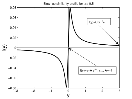
Figure 5. A solutions of (3.2), (3.3) for $\alpha=\frac{1}{2}$ and $A=-1$.

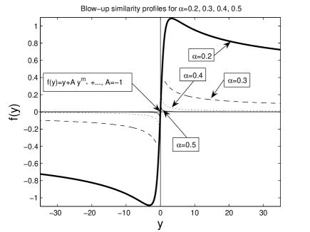
Figure 6. Solutions of (3.2), (3.3) for $\alpha=0.2$, $0.3$, $0.4$, and $0.5$; $A=-1$.

3.1. Rarefaction waves from singular initial data

Similar to (2.21), the global similarity solutions of (1.19),

(3.9) $$\begin{matrix}u_{+}(x,t)=t^{-\alpha}F(y),\quad y=\frac{x}{t^{\beta}}\quad\mbox{for}\quad t>0,\quad\beta=1-\alpha,\qquad\quad\vskip 3.0pt plus 1.0pt minus 1.0pt\vskip 3.0pt plus 1.0pt minus 1.0pt\\ \beta^{2}y^{2}FF^{\prime\prime}=\beta y(F^{\prime})^{2}(\beta y-F)+\beta(\alpha-2)yFF^{\prime}+\alpha F^{2}(-F^{\prime}-1)\quad\mbox{in}\quad\mathbb{R},\qquad\quad\end{matrix}$$

corresponding to the reflection $F\mapsto-F$ in the blow-up ODE (3.2), describe collapse of singular initial data (3.8) posed at $t=0$. We then again arrive at a difficult question on the correct entropy-like choice of proper solutions, which reveal some remnants of those ones for the EEs (1.1) and hyperbolic systems such as (1.3). Hopefully, an evolution entropy test then can be developed in lines of smooth $\delta$-deformations as in [6, 8, 10]. However, there are examples of higher-order PDEs, for which any entropy-like unique extension of a solution after singularity is principally impossible (there are infinitely many extensions that are all equally allowed), [9]. We do not know whether such negative trends can be oriented to the EEs (1.1).

4. Uniqueness of a local continuation after gradient blow-up

We now need to consider the principal question on a generic (self-similar) mechanism of formation of shocks for the model (1.19). To this end, following [9], we will use the same similarity solutions (3.1), but now with

(4.1) $$\textstyle{\alpha<0\quad\Longrightarrow\quad\beta=1-\alpha\equiv 1+|\alpha|>1,\quad\mbox{so that}\quad\frac{|\alpha|}{\beta}\equiv\frac{|\alpha|}{1+|\alpha|}<1.}$$

It can be shown that such solutions (3.1) create continuous “initial data” (cf. (3.8))

(4.2) $$u_{-}(x,0^{-})=\left\{\begin{matrix}\,\,\,C_{0}x^{\frac{|\alpha|}{1+|\alpha|}}\,\,\,\,\,\quad\mbox{for}\quad x>0,\\ -C_{0}|x|^{\frac{|\alpha|}{1+|\alpha|}}\quad\mbox{for}\quad x<0,\end{matrix}\right.$$

where $C_{0}>0$ is some (actually arbitrary by scaling (2.7)) constant. Note that (4.2) is still continuous at $x=0$ but has a first gradient blow-up there.

The question is how to extend the data (4.2) for $t>0$. This is naturally done by using the global similarity solution (3.9). Unlike the previous cases, we here assume that a shock occurs at $y=0$, i.e., we put two conditions there

(4.3) $$F(0)=F_{0}>0\quad\mbox{and}\quad F^{\prime}(0)=F_{1}.$$

By a rather standard local analysis of the ODE (3.9) at $y=0$, it is not difficult to conclude that the Cauchy problem (4.3) has a unique smooth solution in the only case

(4.4) $$\textstyle{F^{\prime}(0)=F_{1}=-1\quad\Longrightarrow\quad F(y)=F_{0}-y+\frac{\beta^{2}y^{2}}{2\alpha F_{0}}+...\,.}$$

For other values of $F^{\prime}(0)\neq-1$, the solution is not smooth and is singular at $y=0$. All such singular bundles can be also derived. Therefore, the behaviour of solution $F(y)$ as $y\to 0^{+}$ is very unstable and, even numerically, its construction is not straightforward.

Before stating the main result, we present in Figure 7 such global similarity profiles $F(y)$ for various values of $\alpha\in[-1,-0.1]$. Since the non-monotonicity of $F(y)$ is not visible here at all, in the next Figure 8, we show typical shape of such profiles in the Cauchy problem posed for $y>\delta=0.1$, with $F(\delta)=1$ and various $F^{\prime}(\delta)<0$. Note that the absolute minimum points at some $y=y_{0}>0$ perfectly corresponds to the Maximum Principle for the ODE (3.9). Indeed, one has:

(4.5) $$F^{\prime}(y_{0})=0,\,\,F(y_{0})>0\quad\Longrightarrow\quad\beta^{2}y_{0}^{2}F(y_{0})F^{\prime\prime}(y_{0})=|\alpha|F^{2}(y_{0})>0.$$

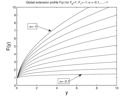
Figure 7. Solutions of the ODE (3.9), (4.4) for $\alpha=-0.1$, $-0.2$,… $-1$.

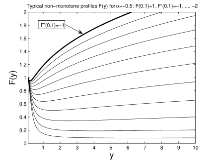
Figure 8. Typical non-monotone solutions of the ODE (3.9), (4.4) for $\alpha=-0.5$.

By checking the asymptotic properties of solutions of (3.9) as $y\to+\infty$, it is not difficult to see that all the profiles with the expansion (4.4), which do not vanish by the Maximum Principle shown in (4.5), exhibit the desired behaviour at infinity:

(4.6) $$F(y)=Cy^{\frac{|\alpha|}{1+|\alpha|}}(1+o(1))\quad\mbox{as}\quad y\to+\infty.$$

Here $C$ is a positive constant but not necessarily the one $C_{0}$ obtained in (4.2) by the blow-up limit. However, the transition $C\mapsto C_{0}$ is uniquely done by the scaling invariance (2.7), so we arrive at:

Proposition 4.1.

For given initial data $\eqref{as4N}$, there exists a unique similarity profile $F(y)$ such that the global similarity solution $\eqref{16NR}$ satisfies

(4.7) $$u_{-}(x,0^{-})=u_{+}(x,0^{+})\quad\mbox{in}\quad\mathbb{R}.$$

We call the corresponding profiles $\{f,F\}$ a similarity global extension pair. Thus, this pair is always unique, so the self-similar blow-up solution $u_{-}(x,t)$ for $t<0$ has a unique extension via the similarity one $u_{+}(x,t)$ for $t>0$.

This justifies a kind of “micro-local” uniqueness theory of shock wave solutions for the PDE (1.19), which sounds rather optimistic. Existence, or even a possibility of construction, of a global “entropy-like” theory for (1.19) (say, in Oleinik–Kruzhkov–Lax–Glimm–Bressan–etc. sense) is quite questionable still. In any case, the above “micro-uniqueness” result is rather inspiring bearing in mind that this could affect some similar extension properties of the EEs.

5. Final conclusions: towards the full model of $(r,\varphi)$-shock and blow-up formation

The integral equation (1.15) assumes another mechanism of shock formation for data:

(5.1) $$V_{0\varphi}\approx 0\quad\mbox{and}\quad V_{0}\approx 1.$$

Then the second term dominates and, on two differentiations, this leads to the PDE:

(5.2) $$U_{r\varphi}=\Big{[}\frac{U_{r\varphi}}{\frac{U}{U_{t}}\big{(}\frac{U_{t}}{U}\big{)}_{t}-U_{r}}\Big{]}_{t}.$$

This equation is supposed to describe more complicated phenomena of shock and more general blow-up formation, where both independent variables $(r,\varphi)$ are essentially and equally involved. Of course, (5.2) is uncomparably more difficult than (1.19), and seems can give a deeper insight into weak and strong singularity formation for the EEs (and also for (1.3)) in the actual 2D $\{r,\varphi\}$-geometry. We do not study this equation here. Nevertheless, it should be mentioned that equations such as (5.2) and others must be carefully investigated and understood before any serious attack of singularity phenomena for Euler equations in 2D and, especially, 3D, which will indeed require other hierarchy of some reduced PDE models to introduce and study.

References

- [1] C. Bardos and E.S. Titi, Euler equations for incompressible ideal fliuds, Russian. Math. Surveys, 62 (2007), 409–451.
- [2] A. Bressan, Hyperbolic Systems of Conservation Laws. The One Dimensional Cauchy Problem, Oxford Univ. Press, Oxford, 2000.
- [3] D. Christodoulou,The Euler equations of compressible fluid flow, Bull. Amer. Math. Soc., 44 (2007), 581–602.
- [4] P. Constantin, On the Euler equations of incompressible fluids, Bull. Amer. Math. Soc., 44 (2007), 603–621.
- [5] C. Dafermos, Hyperbolic Conservation Laws in Continuum Physics, Springer-Verlag, Berlin, 1999.
- [6] V.A. Galaktionov, Nonlinear dispersion equations: smooth deformations, compactons, and extensions to higher orders, Comput. Math. Math. Phys., 48 (2008), 1823–1856 (arXiv:0902.0275).
- [7] V.A. Galaktionov, On blow-up space jets for the Navier–Stokes equations in with convergence to Euler equations, J. Math. Phys., 49 (2008), 113101.
- [8] V.A. Galaktionov, Shock waves and compactons for fifth-order nonlinear dispersion equations, Europ. J. Appl. Math., submitted (arXiv:0902.1632).
- [9] V.A. Galaktionov, Formation of shocks in higher-order nonlinear dispersion PDEs: nonuniqueness and nonexistence of entropy, J. Differ. Equat., submitted (arXiv:0902.1635).
- [10] V.A. Galaktionov and S.I. Pohozaev, Third-order nonlinear dispersion equations: shocks, rarefaction, and blow-up waves, Comput. Math. Math. Phys., 48 (2008), 1784–1810 (arXiv:0902.0253).
- [11] S.N. Kruzhkov, First-order quasilinear equations in several independent variables, Math. USSR Sbornik, 10 (1970), 217–243.
- [12] A.J. Majda and A.L. Bertozzi, Vosticity and Incompressible Flow, Cambridge Univ. Press., Cambridge, 2002.
- [13] K. Ohkitani, A miscellany of basic issues on incompressible fluid equations, Nonlinearity, 21 (2008), T255–T271.
- [14] O.A. Oleinik, Discontinuous solutions of non-linear differential equations, Uspehi Mat. Nauk., 12 (1957), 3–73; Amer. Math. Soc. Transl. (2), 26 (1963), 95–172.
- [15] O.A. Oleinik, Uniqueness and stability of the generalized solution of the Cauchy problem for a quasi-linear equation, Uspehi Mat. Nauk., 14 (1959), 165–170; Amer. Math. Soc. Transl. (2), 33 (1963), 285–290.
- [16] D. Poisson, Mémoire sur la théorie du son, J. Polytech. (14 éme cahier) 7 (1808), 319–392.
- [17] Y. Pomeau, M. Le Berre, P. Guyenne, and S. Grilli, Wave-breaking and generic singularities of nonlinear hyperbolic equations, Nonlinearity, 21 (2008), T61–T79.
- [18] B. Riemann, Über die Fortpfanzung ebener Luftwellen von endlicher Schwingungswete, Abhandlungen der Gesellshaft der Wissenshaften zu Göttingen, Meathematisch-physikalishe Klasse, 8 (1858-59), 43.
- [19] A.A. Samarskii, V.A. Galaktionov, S.P. Kurdyumov, and A.P. Mikhailov, Blow-up in Quasilinear Parabolic Equations, Walter de Gruyter, Belrin/New York, 1995.
- [20] J. Smoller, Shock Waves and Reaction-Diffusion Equations, Springer-Verlag, New York, 1983.
- [21] M.E. Taylor, Partial Differential Equations III. Nonlinear Equations, Springer, New York/Tokyo, 1996.