Finite element methods for a bi-wave equation modeling d-wave superconductors

Abstract

In this paper we develop two conforming finite element methods for a fourth order bi-wave equation arising as a simplified Ginzburg-Landau-type model for $d$-wave superconductors in absence of applied magnetic field. Unlike the biharmonic operator $\Delta^{2}$, the bi-wave operator $\Box^{2}$ is not an elliptic operator, so the energy space for the bi-wave equation is much larger than the energy space for the biharmonic equation. This then makes it possible to construct low order conforming finite elements for the bi-wave equation. However, the existence and construction of such finite elements strongly depends on the mesh. In the paper, we first characterize mesh conditions which allow and not allow construction of low order conforming finite elements for approximating the bi-wave equation. We then construct a cubic and a quartic conforming finite element. It is proved that both elements have the desired approximation properties, and give optimal order error estimates in the energy norm, suboptimal (and optimal in some cases) order error estimates in the $H^{1}$ and $L^{2}$ norm. Finally, numerical experiments are presented to guage the efficiency of the proposed finite element methods and to validate the theoretical error bounds.

1 Introduction

This paper concerns finite approximations of the following boundary value problem:

(1) $$\delta\Box^{2}u-\Delta u =f\qquad \text{in }\Omega,$$

(2) $$u=\partial_{\bar{n}}u =0\qquad \text{on }\partial\Omega,$$

where $0<\delta\ll 1$ is a given (small) number,

$$\Box u :=\partial_{xx}u-\partial_{yy}u,\qquad\qquad\Box^{2}u :=\Box(\Box u),$$

$$\bar{n} :=(n_{1},-n_{2}),\qquad\qquad\partial_{\bar{n}}u :=\nabla u\cdot\overline{n},$$

$\Omega\subset\mathbf{R}^{2}$ is a bounded domain with piecewise smooth boundary $\partial\Omega$, and $n:=(n_{1},n_{2})$ denotes the unit outward normal to $\partial\Omega$. As $\Box$ is the well-known ($2$-D) wave operator, we shall call $\Box^{2}$ the bi-wave operator throughout this paper. It is easy to verify that

$$\Box^{2}u(x,y)=\frac{\partial^{2}u}{\partial x^{2}}-2\frac{\partial^{2}u}{\partial x\partial y}+\frac{\partial^{2}u}{\partial y^{2}}.$$

Hence, equation (1) is a fourth order PDE, which can be viewed as a singular perturbation of the Poisson equation by the bi-wave operator. As a comparison, we recall that the biharmonic operator $\Delta^{2}$ is defined as

$$\Delta^{2}u(x,y):=\Delta(\Delta u(x,y))=\frac{\partial^{2}u}{\partial x^{2}}+2\frac{\partial^{2}u}{\partial x\partial y}+\frac{\partial^{2}u}{\partial y^{2}}.$$

Although there is only a sign difference in the mixed derivative term, the difference between $\Delta^{2}$ and $\Box^{2}$ is fundamental because $\Delta^{2}$ is an elliptic operator while $\Box^{2}$ is a hyperbolic operator.

Superconductors are materials that have no resistance to the flow of electricity when the surrounding temperature is below some critical temperature. At the superconducting state, the electrons are believed to “team up pairwise” despite the fact that the electrons have negative charges and normally repel each other. The Ginzburg-Landau theory [9] has been well accepted as a good mean field theory for low (critical temperature) $T_{c}$ superconductors [11]. However, a theory to explain high $T_{c}$ superconductivity still eludes modern physics. In spite of the lack of satisfactory microscopic theories and models, various generalizations of the Ginzburg-Landau-type models to account for high $T_{c}$ properties such as the anisotropy and the inhomogeneity have been proposed and developed. In low $T_{c}$ superconductors, electrons are thought to pair in a form in which the electrons travel together in spherical orbits, but in opposite directions. Such a form of pairing is often called $s$-wave [11]. However, in high $T_{c}$ superconductors, experiments have produced strong evidence for $d$-wave pairing symmetry in which the electrons travel together in orbits resembling a four-leaf clover (cf. [4, 10, 12, 6] and the references therein). Recently, the $d$-wave pairing has gained substantial support over $s$-wave pairing as the mechanism by which high-temperature superconductivity might be explained. In generalizing the Ginzburg-Landau models to high $T_{c}$ superconductors, the key idea is to introduce multiple order parameters in the Ginzburg-Landau free energy functional. These models, which can also be derived from the phenomenological Gorkov equations [6], have built a reasonable basis upon which detailed studies of the fine vortex structures in some high $T_{c}$ materials have become possible. We refer the reader to [4, 10, 12, 6] and the references therein for a detailed exposition on modeling and analysis of $d$-wave superconductors.

We obtain equation (1) from the Ginzburg-Landau-type $d$-wave model considered in [4] (also see [10, 12]) in absence of applied magnetic field by neglecting the zeroth order nonlinear terms but retaining the leading terms. In the equation, $u$ (notation $\psi_{d}$ is instead used in the cited references) denotes the $d$-wave order parameter. We note that the original order parameter $\psi_{d}$ in the Ginzburg-Landau-type model [10, 4] is a complex-valued scalar function whose magnitude represents the density of superconducting charge carriers, however, to reduce the technicalities and to present the ideas, we assume $u$ is a real-valued scalar function in this paper and remark that the finite element methods developed in this paper can be easily extended to the complex case. We also note that the parameter $\delta$ appears in the full model as $\delta=-\frac{1}{\beta}$, where $\beta$ is proportional to the ratio $\frac{\ln(T_{s0}/T)}{\ln(T_{d0}/T)}$ with $T_{s0}$ and $T_{d0}$ being the critical temperatures of the $s$-wave and $d$-wave components. Clearly, $\beta<0$ (or $\delta>0$) when $T_{s0}<T<T_{d0}$ and $\beta\searrow-\infty$ (or $\delta\searrow 0$) as $T\nearrow T_{d0}$. Hence, $\delta$ is expected to be small for $d$-wave like superconductors.

The primary goal of this paper is to develop conforming finite element methods for the reduced $d$-wave model (1). Since the bi-wave term is the leading term in the full $d$-wave model, see [4, Section 4], any good numerical method for (1) should be applicable to the full $d$-wave model. It is easy to see that the energy space for the bi-wave equation (1) is $V:=\{v\in H^{1}(\Omega);\,\Box v\in L^{2}(\Omega)\}$ (see Section 2). Our main task then is to construct finite element subspaces $V^{h}$ of the energy space $V$ which should be as simple as possible but also rich enough to have good approximation properties. To this end, we note that $H^{2}(\Omega)\subset V\subset H^{1}(\Omega)$, and hence, the desired finite element space $V^{h}$ should satisfy $V^{h}\subset V\subset H^{1}(\Omega)$. This immediately implies that $V^{h}\subset C^{0}(\overline{\Omega})$ (see [3, 2]). On the other hand, since $V$ is a proper subspace of $H^{1}(\Omega)$, the condition $V^{h}\subset C^{0}(\overline{\Omega})$ does not guarantee that $V^{h}\subset V$. Hence, $C^{0}$ (Lagrange) finite element spaces are in general not subspaces of $V$. An intriguing question is what extra conditions are required to make a $C^{0}$ finite element space to be a subspace of $V$. To answer this question, on noting that $H^{2}(\Omega)\subset V$, one may choose $V^{h}$ such that $V^{h}\subset H^{2}(\Omega)$, that is, $V^{h}$ is a $C^{1}$ finite element space such as Argyris finite element space (cf. [3, Chapter 6]). Trivially, $V^{h}\subset H^{2}(\Omega)\subset V$. It turns out (see Section 4) such a choice would work since it can be shown that the finite element solution so defined converges with optimal rate in the energy norm of $V$. However, since $C^{1}$ finite elements require either the use of fifth or higher order polynomials with up to second order derivatives as degrees of freedom [13, 14], or the use of exotic elements [3, Chapter 6], it is expensive and less efficient to solve the bi-wave equation (1) using $C^{1}$ finite elements. This then motivates us to construct low order non-$C^{1}$ finite elements which give genuine subspaces of $V$ and to develop other types of finite element methods such as nonconforming and discontinuous Galerkin methods [7].

The remainder of the paper is organized as follows. Section 2 contains some preliminaries and the functional setting for the bi-wave problem. Well-posedness of the problem and regularity estimates of the weak solution are established. Because $\Box^{2}$ is a hyperbolic operator, the usual regularity shift for fourth order elliptic problems does not hold for the bi-wave problem, instead, a weaker shifting “rule” only holds. Section 3 devotes to construction and analysis of piecewise polynomial subspaces of $V$. First, we give a characterization of such subspaces. It is proved that a subspace of $V$ is “necessarily” a $C^{1}$ finite element space on a general mesh. However, non-$C^{1}$ finite elements are possible on restricted meshes. Second, we construct two such finite elements. The first one is a cubic element and the second is a quartic element. Third, we establish the approximation properties for both proposed finite elements. Because both elements are not affine families, a technique of using affine relatives (cf. [2, 3]) is used to carry out the analysis. Finally, optimal order error estimates in the energy norm of $V$ are proved for the finite element approximations of problem (1)–(2) using the proposed finite elements. Suboptimal (and optimal in some cases) order error estimates in the $L^{2}$-norm are also derived using a duality argument. In Section 4 we present some numerical experiment results to gauge the efficiency of the proposed finite element methods and also to validate our theoretical error bounds.

2 Preliminaries and functional setting

Standard space notation is adopted in this paper. We refer the reader to [2, 3] for their exact definitions. In addition, $(\cdot,\cdot)$ and $\langle\cdot,\cdot\rangle_{\partial\Omega}$ are used to denote the $L^{2}$-inner products on $\Omega$ and on $\partial\Omega$, respectively. $C$ denotes a generic $h$ and $\delta$-independent positive constant. We also introduce the following special space notation:

$$V_{0}:=\{v\in V\cap H^{1}_{0}(\Omega);\ \partial_{\bar{n}}v\big{|}_{\partial\Omega}=0\}, \qquad(v,w)_{V}:=\delta(\Box u,\Box w)+(v,w),$$

$$\|v\|_{V}:=\sqrt{(v,v)_{V}}.$$

It is easy to verify that $(\cdot,\cdot)_{V}$ is an inner product on $V$, hence, $\|\cdot\|_{V}$ is the induced norm, and $V$ endowed with this inner product is a Hilbert space. We remark that all above claims do not hold in general if the harmonic term $\Delta u$ is dropped in (1) because the kernels of the bi-wave operator $\Box^{2}$ and the wave operator $\Box$ may contain non-zero functions satisfying the homogeneous Dirichlet boundary condition [1].

The variational formulation of (1)–(2) can be derived easily by testing (1) against a test function $v\in V_{0}$ and using integration by parts formulas. Specifically, it is defined as seeking $u\in V_{0}$ such that

(3) $$A^{\delta}(u,v)=\langle f,v\rangle,$$

where

$$A^{\delta}(u,v):=(u,v)_{V},$$

and $\langle\cdot,\cdot\rangle$ denotes the pairing between $V$ and its dual, $V^{*}$.

We now show that problem (3) is well-posed.

Theorem 2.1.

For any $f\in V^{*}$, there exists a unique solution to (3). Furthermore, there holds estimate

(4) $$\|u\|_{V}\leq\|f\|_{V^{*}}.$$

Proof.

We note for $v,w\in V_{0}$,

(5) $$A^{\delta}(v,v) \geq\|v\|_{V}^{2},$$

(6) $$|A^{\delta}(v,w)\big{|} \leq\|v\|_{V}\|w\|_{V}.$$

Then, existence and uniqueness follows directly from an application of the Lax-Milgram Theorem (cf. [2, 3]) and using the fact that $V_{0}$ is a Hilbert space with the inner product $(\cdot,\cdot)_{V}$. The estimate (4) follows from (5) and (3) after setting $v=u$ and $w=u$. ∎

We note $H^{2}(\Omega)$ is a proper subspace of $V$, so in general $u\not\in H^{2}(\Omega)$ if $f\in V^{*}$. However, for smoother function $f$ we have the following regularity results.

Theorem 2.2.

Assume that the boundary $\partial\Omega$ of the domain $\Omega$ is sufficiently smooth. Let $s_{1},s_{2}$ be two nonnegative integers. Then there exist constants $C_{s_{1},s_{2}},\hat{C}_{s_{1},s_{2}}>0$ such that the weak solution $u$ of (3) satisfies

(7) $$\|\partial^{s_{1}}_{x}\partial^{s_{2}}_{y}u\|_{V}\leq C_{s_{1},s_{2}}\|\partial^{s_{1}}_{x}\partial^{s_{2}}_{y}f\|_{V^{*}} \qquad\mbox{if }\partial^{s_{1}}_{x}\partial^{s_{2}}_{y}f\in V^{*},$$

$$\sqrt{\delta}\|\Box^{2}\partial^{s_{1}}_{x}\partial^{s_{2}}_{y}u\|_{L^{2}}+\sqrt{\delta}\|\nabla\Box\partial^{s_{1}}_{x}\partial^{s_{2}}_{y}u\|_{L^{2}}$$

(8) $$+\|\Delta\partial^{s_{1}}_{x}\partial^{s_{2}}_{y}u\|_{L^{2}}\leq \hat{C}_{s_{1},s_{2}}\|\partial^{s_{1}}_{x}\partial^{s_{2}}_{y}f\|_{L^{2}} \qquad\mbox{if }\partial^{s_{1}}_{x}\partial^{s_{2}}_{y}f\in L^{2}(\Omega).$$

Proof.

First, we consider the case that $u$ and $f$ have compact support. Let $w:=\partial^{s_{1}}_{x}\partial^{s_{2}}_{y}u$ and $g:=\partial^{s_{1}}_{x}\partial^{s_{2}}_{y}f$. Because equation (1) is a linear equation, differentiating the equation immediately verifies that $w$ and $g$ satisfy

(9) $$\delta\Box^{2}w-\Delta w=g,$$

that is, $w$ is a solution of the bi-wave equation with the source term $g$. Since $u$ is assumed to have a compact support, then $w$ also satisfies the homogeneous boundary conditions in (2). Thus, it follows from Theorem 2.1 that

$$\|w\|_{V}\leq\|g\|_{V^{*}},$$

which gives (7) with $C_{s_{1},s_{2}}=1$.

To show (8), it suffices to prove that

(10) $$\sqrt{\delta}\|\nabla\Box w\|_{L^{2}}+\|\Delta w\|_{L^{2}}\leq\hat{C}_{s_{1},s_{2}}\|g\|_{L^{2}},$$

which is equivalent to prove that (8) holds for $s_{1}=s_{2}=0$. To this end, testing (9) with $-\Delta w$ yields

$$-\delta(\Box^{2}w,\Delta w)+\|\Delta w\|_{L^{2}}^{2}=-(g,\Delta w).$$

Using the following integral identity

$$(\Box^{2}\varphi,\psi)_{\Omega}=\langle\partial_{\bar{n}}\Box\varphi,\psi\rangle_{\partial\Omega}-\langle\Box\varphi,\partial_{\bar{n}}\psi\rangle_{\partial\Omega}+(\Box\varphi,\Box\psi)_{\Omega}$$

followed by using Green’s identity (for $\Delta$) in the first term on the left hand side we get

$$-\delta(\Box^{2}w,\Delta w)=\delta\|\nabla\Box w\|_{L^{2}}^{2}.$$

Here, we have dropped the boundary integral terms because $w$ has a compact support.

Combining the above two identities for $w$ and using Schwarz inequality yield

$$\delta\|\nabla\Box w\|_{L^{2}}^{2}+\|\Delta w\|_{L^{2}}^{2}\leq\frac{1}{2}\|g\|_{L^{2}}^{2}+\frac{1}{2}\|\Delta w\|_{L^{2}}^{2}.$$

Hence, the above inequality and (9) imply that (10) holds with $\hat{C}_{s_{1},s_{2}}=2\sqrt{2}+1$.

Second, in the case $u$ and $f$ do not have compact support, it is clear that $w$ and $g$ still satisfy (9). However, $w$ and its derivatives may not satisfy the homogeneous boundary conditions in (2). To get around this difficulty, the well-known tricks are to use the cutoff function technique (see [5, 8]) for interior estimates and to use the flattening boundary technique for boundary estimates. The cutoff function technique involves testing (9) by $w\xi$ and $-\Delta w\xi$, instead of $w$ and $-\Delta w$, for a smooth cutoff function $\xi$. Integrating by parts on the left hand side and using Schwarz inequality and the properties of the cutoff function then yield the desired interior estimate similar to (7) and (8). The flattening boundary technique involves locally mapping the curved boundary into a flat boundary by a smooth map (this requires the smoothness of the boundary $\partial\Omega$). After the desired boundary estimates are obtained in the new coordinates, they are then transferred to the solution $w$ in the original coordinates. We omit the technical derivations and refer the interested reader to [5, 8] for a detailed exposition of these techniques applying to other linear PDEs. ∎

3 Construction and analysis of finite element methods

3.1 Characterization of finite element subspaces of $V$

Let $\mathcal{T}_{h}$ be a quasi-uniform triangulation of $\Omega$ with mesh size $h\in(0,1)$, and for a fixed $T\in\mathcal{T}_{h}$, let $(\lambda_{1}^{T},\lambda_{2}^{T},\lambda_{3}^{T})$ denote the barycentric coordinates, and $a_{i}\ (1\leq i\leq 3)$ denote the vertices of $T$. We also let $e_{i}\ (1\leq i\leq 3)$ denote the edge of $T$ of which $a_{i}$ is not a vertex, and $b_{i}$ denote the midpoint of edge $e_{i}$. Define the interior and boundary edge sets of $\mathcal{T}_{h}$

$$\mathcal{E}_{h}^{I}: =\{e;\ e\cap\partial\Omega=\emptyset\},\qquad\mathcal{E}_{h}^{B}:=\{e;\ e\cap\partial\Omega\neq\emptyset\}.$$

We also set

$$\mathcal{E}_{h}:=\mathcal{E}_{h}^{I}\cup\mathcal{E}_{h}^{B},$$

and for $T\in\mathcal{T}_{h}$,

$$\omega(T):=\mbox{closure}\left(\bigcup_{\partial T^{\prime}\cap\partial T\neq\emptyset}T^{\prime}\right).$$

For any $e\in\mathcal{E}_{h}^{I}$ such that $e=T_{1}\cap T_{2}$, and $v\in H^{1}(T_{1})\cap H^{1}(T_{2})$, define the jumps of $v$ across $e$ as (assuming the global label of $T_{1}$ is bigger than that of $T_{2}$)

$$[v]\big{|}_{e}:=v^{T_{1}}\big{|}_{e}-v^{T_{2}}\big{|}_{e},$$

where $v^{T_{i}}=v\big{|}_{T_{i}}$, and $[v]\big{|}_{e}:=v^{T_{1}}\big{|}_{e}$ if $e\in\mathcal{E}_{h}^{B}$.

Similarly, for $v\in H^{2}(T_{1})\cap H^{2}(T_{2}),\ \alpha\in\mathbf{R}^{2}$, we define the jumps of $\partial_{\alpha}v:=\nabla v\cdot\alpha$ as follows:

$$[\partial_{\alpha}v]\big{|}_{e} :=\partial_{\alpha}v^{T_{1}}\big{|}_{e}-\partial_{\alpha}v^{T_{2}}\big{|}_{e}\qquad e=\partial T_{1}\cap\partial T_{2}\in\mathcal{E}^{I}_{h},$$

$$[\partial_{\alpha}v]\big{|}_{e} :=\partial_{\alpha}v^{T_{1}}\big{|}_{e}\qquad e=\partial T_{1}\cap\partial\Omega\in\mathcal{E}_{h}^{B}.$$

We also define the shorthand notation

$$\overline{\nabla}v:=(v_{x},-v_{y}),\qquad\overline{|\nabla v|}:=\nabla v\cdot\overline{\nabla}v.$$

In the rest of the paper, we shall often encounter the following characterization of the meshes.

Definition 1.

For $e\in\mathcal{E}_{h}$, let $n$ and $\tau$ denote the outward unit normal and unit tangent vector of $e$, respectively. We say that $e$ is a type I edge if

(11) $$\overline{n}=\tau\quad\text{or}\quad\overline{n}=-\tau.$$

Otherwise, $e$ is called a type II edge if condition (11) does not hold.

Remark 3.1.

(a) If $e$ is a type I edge, then $\overline{n}=(n_{1},-n_{2})=\pm\tau=\pm(\tau_{1},\tau_{2})=\pm(n_{2},-n_{1})$. Therefore,

$$\tau=\frac{\sqrt{2}}{2}(\pm 1,\pm 1).$$

That is, the edge $e$ makes an angle of $\frac{\pi}{4}$ in the plane with respect to the $x$-axis. Examples of meshes such that every triangle in the partition has exactly zero and one type I edges are shown in Figure 1, and examples of meshes such that every triangle has exactly two type I edges are shown in Figure 2.

(b) For $T\in\mathcal{T}_{h}$, $e_{i}\subset\partial T$, let $n^{(i)}$ and $\tau^{(i)}$ denote the outward (from $T$) unit normal and unit tangent vector of $e_{i}$, respectively. Then using the formula

$$n^{(i)}=-\frac{\nabla\lambda^{T}_{i}}{\|\nabla\lambda^{T}_{i}\|},$$

we conclude that $e_{i}$ is a type I edge if and only if

$$\nabla\lambda^{T}_{i}\cdot\overline{\nabla}\lambda^{T}_{i}=0.$$

   

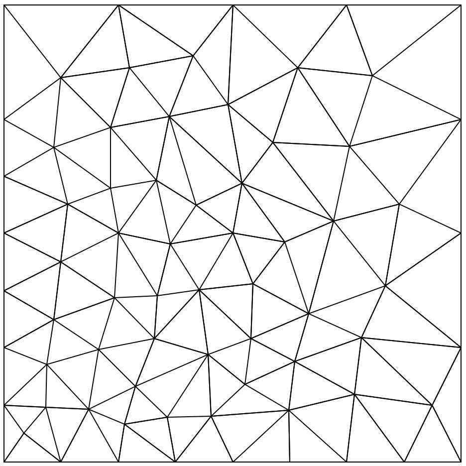
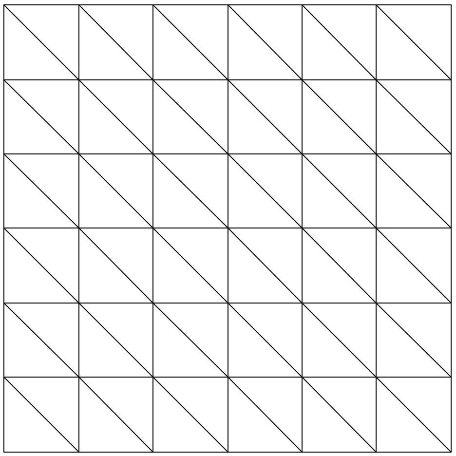
Fig. 1: Example of meshes of the domain $\Omega=(0,1)^{2}$ such that every triangle has no type I edges (left), and one type I edge (right).

   

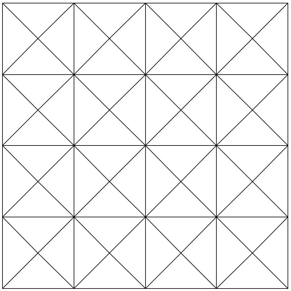
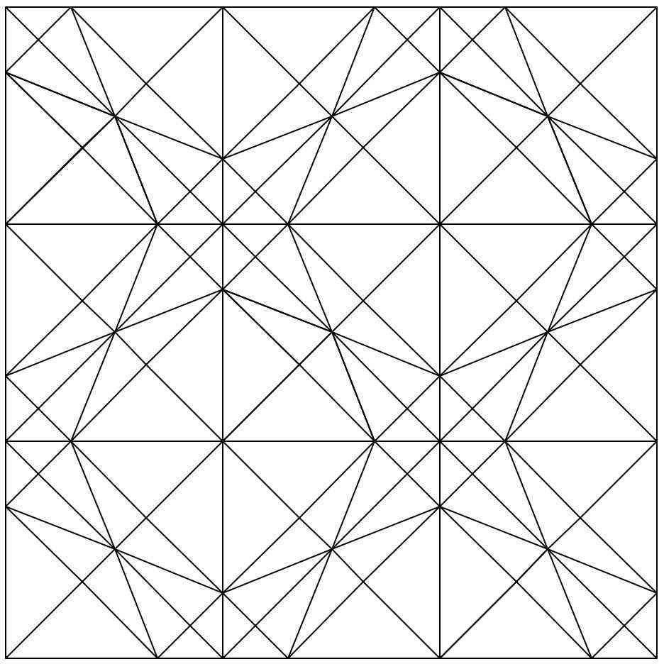
Fig. 2: Example of a uniform mesh (left) and a nonuniform mesh (right) of the domain $\Omega=(0,1)^{2}$ such that every triangle has two type I edges.

To construct finite element subspaces of $V$, we first provide the following two lemmas, which characterize such spaces.

Lemma 3.2.

Let $X^{h}$ be a subspace of $V$ consisting of piecewise polynomials, and suppose there exists a type II edge $e\in\mathcal{E}_{h}^{I}$ with $e=\partial T_{1}\cap\partial T_{2}$. Then for $v\in X^{h}$, there holds the inclusion $v\in H^{2}(T_{1}\cup T_{2})$.

Proof.

Since $X^{h}$ is finite-dimensional with $X^{h}\subset H^{1}(\Omega)$, we have the inclusion $X^{h}\subset C^{0}(\overline{\Omega})$. We also note that it suffices to show $v\in C^{1}(\overline{T}_{1}\cup\overline{T}_{2})$ for any $v\in X_{h}$, which in turn is equivalent to show

$$\big{[}\partial_{\alpha}v\big{]}\big{|}_{e}=0\qquad\forall\alpha\in\mathbf{R}^{2}.$$

Let $n$ and $\tau$ denote the normal and tangential direction of $e$, respectively. Rewriting $V$ as

$$V=\{v\in H^{1}(\Omega);\ \overline{\nabla}v\in H({\rm div};\Omega)\},$$

there holds for $v\in X^{h}$

$$\big{[}\partial_{\bar{n}}v\big{]}\big{|}_{e}=0.$$

Next, using the assumption $\overline{n}\neq\pm\tau$, we can write for any constant vector $\alpha\in\mathbf{R}^{2}$

$$\big{[}\partial_{\alpha}v\big{]}\big{|}_{e}=\frac{1}{1-(\tau\cdot\overline{n})^{2}}\Big{\{}\alpha\cdot\big{(}\tau-\overline{n}(\tau\cdot\overline{n})\big{)}\big{[}\partial_{\tau}v]\Big{|}_{e}+\alpha\cdot\big{(}\overline{n}-\tau(\tau\cdot\overline{n})\big{)}\big{[}\partial_{\bar{n}}v\big{]}\Big{|}_{e}\Big{\}}.$$

But $\big{[}\partial_{\tau}v\big{]}\big{|}_{e}=0$ since $v\in C^{0}(\overline{\Omega})$ and $v\big{|}_{e}$ is a polynomial of one variable. Hence, $\big{[}\partial_{\bar{n}}v\big{]}\big{|}_{e}=0$ implies that $\big{[}\partial_{\alpha}v\big{]}\big{|}_{e}=0$. The proof is complete. ∎

Corollary 3.3.

Suppose $X^{h}$ is a subspace of $V$ consisting of piecewise polynomials, and suppose there exists no type I edges in the set $\mathcal{E}_{h}^{I}$. Then $X^{h}\subset H^{2}(\Omega)$.

Lemma 3.4.

Suppose $\Sigma_{T}$ is a linearly independent set of parameters uniquely determining a $k$th-degree polynomial $v$ on an interior triangle $T\in\mathcal{T}_{h}$ that includes only function and derivative degrees of freedom. Suppose further that $v$ is continuous in $\omega(T)$, $\Box v\in L^{2}(\omega(T))$, and $T$ has at least two type II edges that are in the set $\mathcal{E}_{h}^{I}$. Then $k\geq 5$.

Proof.

If $T$ has three type II edges, then by Lemma 3.2, $v\in H^{2}(\omega(T))$, and it follows that $k\geq 5$ (cf. [3, p.108], also see [13, 14]).

Suppose $T$ has exactly two type II edges, without loss of generality, assume $e_{1}$ is type I. By the proof of Lemma 3.2, $v$ is $C^{1}$ across edges $e_{2}$ and $e_{3}$. Let $\mu_{i}$ denote the order of prescribed derivatives at vertex $a_{i}$ in the set $\Sigma_{T}$, let $m_{i}$ denote the number of function value (or equivalent) degrees of freedom in the set $\Sigma_{T}$ on edge $e_{i}$, and let $s_{i}$ denote the number of (non-tangential) directional derivative value (or equivalent) degrees of freedom in the set $\Sigma_{T}$ on edge $e_{i}$. Since $v$ is continuous in $\omega(T)$, we have

(12) $$\mu_{2}+\mu_{3}+m_{1} \geq k-1,$$

$$\mu_{1}+\mu_{3}+m_{2} \geq k-1,$$

$$\mu_{1}+\mu_{2}+m_{3} \geq k-1,$$

and since $\nabla v$ is continuous across $e_{2}$ and $e_{3}$,

(13) $$\mu_{1}+\mu_{2}+s_{3} \geq k,$$

$$\mu_{1}+\mu_{3}+s_{2} \geq k.$$

Adding up the above five inequalities yields

$$4\mu_{1}+3\mu_{2}+3\mu_{3}+m_{1}+m_{2}+m_{3}+s_{1}+s_{2}\geq 5k-3.$$

Because the set $\Sigma_{T}$ is linearly independent, and the dimension of $\Sigma_{T}$ equals $\frac{(k+1)(k+2)}{2}$, there holds

(14) $$\frac{(k+1)(k+2)}{2} \geq\sum_{i=1}^{3}\Big{\{}\frac{1}{2}(\mu_{i}+1)(\mu_{i}+2)+m_{i}\Big{\}}+s_{2}+s_{3}$$

$$\geq\sum_{i=1}^{3}\frac{1}{2}(\mu_{i}+1)(\mu_{i}+2)+5k-3-4\mu_{1}-3\mu_{2}-3\mu_{3}.$$

Thus,

(15) $$(k^{2}-7k+8) \geq(\mu_{1}^{2}-5\mu_{1}+2)+(\mu_{2}-2)(\mu_{2}-1)+(\mu_{3}-2)(\mu_{3}-1).$$

It is clear that $k$ must be greater than two, therefore, it suffices to show that $k$ cannot equal three or four.

Case $k=3$: If $k=3$, by (15) we get

$$(\mu_{1}-3)(\mu_{1}-2)+(\mu_{2}-2)(\mu_{2}-1)+(\mu_{3}-2)(\mu_{3}-1)\leq 0,$$

and since $\mu_{i}$ are integer-valued, we have

$$1\leq\mu_{3}\leq 2,\quad 1\leq\mu_{2}\leq 2,\quad 2\leq\mu_{1}\leq 3.$$

But by (14), we immediately obtain

$$10=\frac{(k+1)(k+2)}{2}\geq\sum_{i=1}^{3}\frac{1}{2}(\mu_{i}+1)(\mu_{i}+2)\geq 12,$$

which is a contradiction.

Case $k=4$: As in the previous case, if $k=4$ we have

$$(\mu_{1}-3)(\mu_{1}-2)+(\mu_{2}-2)(\mu_{2}-1)+(\mu_{3}-2)(\mu_{3}-1)\leq 0.$$

Since

$$1\leq\mu_{3}\leq 2,\quad 1\leq\mu_{2}\leq 2,\quad 2\leq\mu_{1}\leq 3,$$

and

$$15=\frac{(k+1)(k+2)}{2}\geq\sum_{i=1}^{3}\frac{1}{2}(\mu_{i}+1)(\mu_{i}+2),$$

it is not hard to check that there can only be the following three subcases:

(16) $$(\mu_{1},\mu_{2},\mu_{3})=(2,1,2),\quad(\mu_{1},\mu_{2},\mu_{3})=(2,2,1),\quad(\mu_{1},\mu_{2},\mu_{3})=(2,1,1).$$

If the first subcase holds, then all degrees of freedom lie on the vertices, therefore, $m_{i},s_{i}=0,\ 1\leq i\leq 3$. However, it follows from (13) that

$$3=\mu_{1}+\mu_{2}\geq 4,$$

which is a contradiction.

A similar argument can be used to exclude the second subcase in (16). Now, suppose $\mu_{1}=2,\ \mu_{2}=1,$ and $\mu_{3}=1$. By (12) and (13), we have

$$m_{3}\geq 1,\qquad s_{3}\geq 2,\qquad s_{2}\geq 1.$$

But this implies that

$$15\geq\sum_{i=1}^{3}\big{\{}\frac{1}{2}(\mu_{i}+1)(\mu_{i}+2)+m_{i}\big{\}}+s_{2}+s_{3}\geq 16,$$

a contradiction. Thus, the third subcase can not happen, either. Therefore, we must have $k\geq 5$. The proof is complete. ∎

By Lemmas 3.2 and 3.4, and Corollary 3.3, we conclude that unless certain types of meshes are used, we must resort to either $C^{1}$ finite elements such as Argyris, Hsieh-Clough-Tocher, Bogner-Fox-Schmit elements (cf. [2, 3]), or special exotic elements (e.g. macro elements), or nonconforming elements (cf. [7]) to solve problem (1)–(2), However for special meshes, we now show in the following subsections that it is feasible to construct low order finite element subspaces of $V$.

3.2 A cubic conforming finite element

To construct a cubic conforming finite element, we assume that $\mathcal{T}_{h}$ is a triangulation of $\Omega$ and every triangle of $\mathcal{T}_{h}$ has two type I edges. Examples of such meshes are shown on a square domain in Figure 2. Our cubic finite element $S^{h}_{3}:=(T,P_{T},\Sigma_{T})$ is defined as follows:

1. $T$ is a triangle with two type I edges,

2. $P_{T}=\mathbb{P}_{3}(T)$, the space of cubic polynomials on $T$,

3. $\displaystyle{\Sigma_{T}=\left\{\begin{array}[]{ll}v(a_{i})&1\leq i\leq 3,\\ v(a_{i3})&1\leq i\leq 2,\\ \nabla v(a_{i})\cdot(a_{j}-a_{i})&1\leq i\leq 2,\ 1\leq j\leq 3,\ j\neq i,\\ \partial_{\bar{n}}v(b_{3}),\end{array}\right.}$

   where $e_{3}$ is a type II edge.

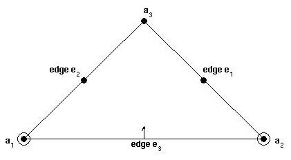
Fig. 3: Element $S^{h}_{3}$. Solid dots indicate function evaluation, circles indicate first derivative evaluation, and arrows indicate evaluation of derivatives in the direction $\overline{n}$.

Lemma 3.5.

The set $\Sigma_{T}$ is unisolvent. That is, any polynomial of degree three is uniquely determined by the degrees of freedom in $\Sigma_{T}$.

Proof.

Suppose $v\in\mathbb{P}_{3}(T)$ equals zero at all the degrees of freedom in $\Sigma_{T}$. To complete the proof, it suffices to show $v\equiv 0$ since dim($\mathbb{P}_{3}(T))=\text{dim}(\Sigma_{T})=10$.

Recall that $e_{3}$ is a type II edge, $e_{1}$ and $e_{2}$ are type I edges of $T$. Let $w_{i}$ be the restriction of $v$ on $e_{i}\subset\partial T$ as a function of a single variable, then $w_{i}$ is a polynomial of degree three which satisfies

$$w_{i}^{\prime}(0)=w_{i}(0)=w_{i}(\frac{1}{2})=w_{i}(1)=0\qquad i=1,2,$$

$$w^{\prime}_{3}(0)=w_{3}(0)=w_{3}(1)=w_{3}^{\prime}(1)=0.$$

In either case, we conclude $w_{i}\equiv 0$.

Next, let $z_{3}$ be the restriction of $\partial_{\bar{n}}v$ on $e_{3}$ as a function of a single variable. Then $z_{3}$ is a polynomial of degree two satisfying

$$z_{3}(0)=z_{3}(\frac{1}{2})=z_{3}(1),$$

which then infers $z_{3}\equiv 0$.

From the above calculations, we conclude that $(\lambda_{3}^{T})^{2}$, $\lambda_{1}^{T}$, and $\lambda_{2}^{T}$ are factors of $v$. However, this is not possible, since $v$ is a polynomial of degree three, unless $v\equiv 0$. The proof is complete. ∎

Let $V^{h}_{3}$ be the finite element space associated with $S_{3}^{h}$, that is,

$$V^{h}_{3}=\{v|_{T}\in\mathbb{P}_{3}(T),\,v\mbox{ is continuous at every degree of freedom in }\Sigma_{T},\,\forall T\in\mathcal{T}_{h}\}.$$

We now show that $V^{h}_{3}$ is a subspace of $V$.

Theorem 3.6.

There holds the inclusion $V^{h}_{3}\subset V$.

Proof.

Let $v\in V^{h}_{3}$. By the proof of Lemma 3.2, it suffices to show $v$ and $\partial_{\bar{n}}v$ are both continuous across interior edges of $\mathcal{T}_{h}$. Let $T_{1}$ and $T_{2}$ be two adjacent triangles with common edge $e$, and $w$ be the restriction of $v^{T_{1}}-v^{T_{2}}$ along $e$ as a function of a single variable. We then have

$$w^{\prime}(0)=w_{1}(0)=w(\frac{1}{2})=w(1)=0\qquad \text{if $e$ is type I},$$

$$w^{\prime}(0)=w(0)=w(1)=w^{\prime}(1)=0\qquad \text{if $e$ is type II}.$$

Thus, $w\equiv 0$ and the inclusion $V^{h}_{3}\subset C^{0}(\Omega)\subset H^{1}(\Omega)$ holds.

Next, we observe that if $e$ is a type I edge, then

$$\big{[}\partial_{\bar{n}}v\big{]}\big{|}_{e}=\pm\big{[}\partial_{\tau}v\big{]}\big{|}_{e}=0.$$

Hence, $\partial_{\bar{n}}v$ is continuous across $e$. On the other hand, if $e$ is a type II edge, let $z$ be the restriction of $[\partial_{\bar{n}}v]|_{e}=\partial_{\bar{n}}v^{T_{1}}-\partial_{\bar{n}}v^{T_{2}}$ along $e$ as a function of a single variable. Since

$$z(0)=z(\frac{1}{2})=z(1),$$

and $z$ is a polynomial of degree two, it follow that $\big{[}\partial_{\bar{n}}v\big{]}\big{|}_{e}=0$. So $\partial_{\bar{n}}v$ is also continuous across $e$. This then concludes the proof. ∎

Remark 3.7.

We note that $V^{h}_{3}\not\subset H^{2}(\Omega)$ because $V^{h}_{3}\not\subset C^{1}(\Omega)$.

3.3 A quartic conforming finite element

In this subsection, we again assume that $\mathcal{T}_{h}$ is a triangulation of $\Omega$ and every triangle of $\mathcal{T}_{h}$ has two type I edges. We then define the following quartic finite element $S_{4}^{h}:=(T,Q_{T},\Xi_{T})$:

1. $T$ is a triangle with two type I edges,

2. $Q_{T}=\mathbb{P}_{4}(T)$, the space of quartic polynomials on $T$,

3. $\displaystyle{\Xi_{T}=\left\{\begin{array}[]{ll}v(a_{i})&1\leq i\leq 3,\\ v(a_{ii3}),\,v(a_{i33})&1\leq i\leq 2,\\ v(b_{3}),\\ v(a_{123}),\\ \nabla v(a_{i})(a_{j}-a_{i})&1\leq i\leq 2,\ 1\leq j\leq 3,\ j\neq i,\\ \partial_{\bar{n}}v(a_{112}),\,\partial_{\bar{n}}v(a_{122}),\end{array}\right.}$

   where $e_{3}$ is a type II edge, and $a_{ij\ell}=\frac{1}{3}\big{(}a_{i}+a_{j}+a_{\ell})$.

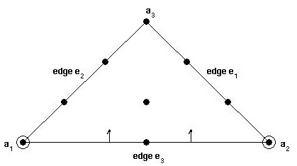
Fig. 4: Element $S^{h}_{4}$. Solid dots indicate function evaluation, circles indicate first derivative evaluation, and arrows indicate evaluation of derivatives in the direction $\overline{n}$.

Lemma 3.8.

The set $\Xi_{T}$ is unisolvent. That is, any polynomial of degree four is uniquely determined by the degrees of freedom in $\Xi_{T}$.

Proof.

Suppose $v\in\mathbb{P}_{4}(T)$ equals zero at all the degrees of freedom in $\Xi_{T}$, and let $w_{i}$ be the restriction of $v$ to $e_{i}$ as a function of a single variable. Then

$$w_{i}^{\prime}(0)=w_{i}(0)=w_{i}(\frac{1}{3})=w_{i}(\frac{2}{3})=w_{i}(1)=0\qquad i=1,2,$$

$$w_{3}^{\prime}(0)=w_{3}(0)=w_{3}(\frac{1}{2})=w_{3}(1)=w_{3}^{\prime}(1)=0.$$

Thus, $w_{i}\equiv 0,i=1,2,3$.

Next, letting $z_{3}$ be the restriction of $\partial_{\bar{n}}v$ on $e_{3}$ as a function of a single variable, we have

$$z_{3}(0)=z_{3}(\frac{1}{3})=z_{3}(\frac{2}{3})=z_{3}(1)=0.$$

Hence, $z_{3}\equiv 0$.

From the above calculations, we conclude that $v=a\lambda_{1}\lambda_{2}\lambda_{3}^{2}$ for some $a\in\mathbf{R}$. However, since $0=v(a_{123})=\frac{a}{81}$, we have $a=0$. The proof is complete. ∎

Theorem 3.9.

Let $V^{h}_{4}$ be the finite element space associated with $S_{4}^{h}$, that is,

$$V^{h}_{4}=\{v|_{T}\in\mathbb{P}_{4}(T),\,v\mbox{ \rm is continuous at every degree of freedom in }\Xi_{T},\,\forall T\in\mathcal{T}_{h}\}.$$

Then there holds the inclusion $V^{h}_{4}\subset V$.

Proof.

Let $v\in V^{h}_{4}$, and suppose $T^{1},T^{2}\in\mathcal{T}_{h}$ are two adjacent triangles with common edge $e$. Let $w$ be the restriction of $[v]|_{e}=v^{T_{1}}-v^{T_{2}}$ along $e$ as a function of a single variable, from

$$w^{\prime}(0)=w(0)=w(\frac{1}{3})=w(\frac{2}{3})=w(1)=0\qquad \text{if $e$ is type I},$$

$$w^{\prime}(0)=w(0)=w(\frac{1}{2})=w(1)=w^{\prime}(1)=0\qquad \text{if $e$ is type II},$$

we conclude $w\equiv 0$. Hence, the inclusion $V^{h}_{4}\subset C^{0}(\Omega)\subset H^{1}(\Omega)$ holds.

If $e$ is a type II edge, we let $z$ denote the restriction of $[\partial_{\bar{n}}v]|_{e}=\partial_{\bar{n}}v^{T_{1}}-\partial_{\bar{n}}v^{T_{2}}$ along $e$ as a function of one variable. It follows from

$$z(0)=z(\frac{1}{3})=z(\frac{2}{3})=z(1)=0,$$

that $z\equiv 0$.

Finally, if $e$ is a type I edge, we use the fact that $v$ is continuous to conclude

$$\big{[}\partial_{\bar{n}}v\big{]}\big{|}_{e}=\pm\big{[}\partial_{\tau}v\big{]}\big{|}_{e}=0.$$

Thus, $V_{4}^{h}\subset V$. ∎

Remark 3.10.

We note that $V^{h}_{4}\not\subset H^{2}(\Omega)$ because $V^{h}_{4}\not\subset C^{1}(\Omega)$.

3.4 Approximation properties of the proposed finite elements

Let $\Pi^{T}_{k}v\in\mathbb{P}_{k}(T)$ denote the standard interpolation of $v$ associated with the finite element $S^{h}_{k}$, and define $\Pi^{h}_{k}v\in V_{k}^{h}$ such that $\Pi^{h}_{k}v\big{|}_{T}=\Pi_{k}^{T}(v\big{|}_{T}),\ \forall T\in\mathcal{T}_{h}$. Before stating the approximation properties of the interpolation operator $\Pi_{k}^{T}$, we first establish the following technical lemma concerning the mesh $\mathcal{T}_{h}$.

Lemma 3.11.

Suppose $T\in\mathcal{T}_{h}$ has two type I edges, and without loss of generality, assume $e_{3}\subset\partial T$ is a type II edge. Then there exists a constant $C>0$ that depends only on the minimum angle of $T$ such that

$$1-\big{(}\beta^{(3)}\big{)}^{2}\geq C,$$

where $\beta^{(3)}=\tau^{(3)}\cdot\overline{n}^{(3)}$.

Proof.

Since both type I edges of $T$ make an angle of $\frac{\pi}{4}$ with respect to the $x$-axis (cf. Remark 3.1), then there exists $\theta\in(0,\frac{\pi}{4}]$ such that the angles of $T$ are $\frac{\pi}{2},\ \theta$, and $\frac{\pi}{2}-\theta$.

Next, we embed $T$ into an isosceles triangle as shown in Figure 5,

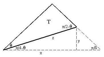
Fig. 5: Embedding $T$ into an isosceles triangle

and then obtain

$$\tau^{(3)}=\frac{(x,y)}{z},\quad\tau^{(3)}\cdot\overline{n}^{(3)}=\frac{-2xy}{z^{2}},\quad x=\cos(\frac{\pi}{4}-\theta)z,\quad y=\sin(\frac{\pi}{4}-\theta)z.$$

Hence,

$$\tau^{(3)}\cdot\overline{n}^{(3)} =\frac{-2xy}{z^{2}}=-2\sin(\frac{\pi}{4}-\theta)\cos(\frac{\pi}{4}-\theta)=-\cos(2\theta),$$

which implies that

$$1-(\beta^{(3)})^{2}=1-(\tau^{(3)}\cdot\overline{n}^{(3)})^{2}=1-\cos^{2}(2\theta)=\sin^{2}(2\theta).$$

The proof is complete. ∎

Remark 3.12.

If $\mathcal{T}_{h}$ is a uniform criss-cross triangulation of $\Omega$, then $1-(\beta^{(3)})^{2}=1$ for all type II edges, $e_{3}$.

The next theorem establishes the approximation properties of the proposed cubic and quartic finite elements.

Theorem 3.13.

For all $m\geq 0$, $p,q\in[1,\infty]$ which are compatible with the inclusion

$$W^{k+1,p}(T) \hookrightarrow W^{m,q}(T),$$

there holds

(17) $$\|v-\Pi^{T}_{k}v\|_{W^{m,q}(T)}\leq Ch_{T}^{k+1-m+\frac{2}{q}-\frac{2}{p}}\|v\|_{W^{k+1,p}(T)}\qquad\forall v\in W^{k+1,p}(T),$$

where $h_{T}={\rm diam}(T)$.

Proof.

The case $S^{h}_{3}$: Since $S^{h}_{3}$ is not an affine family in general, the standard scaling technique can not be used directly to prove (17). To get around this difficulty, the trick is to introduce an affine “relative” of $S^{h}_{3}$ and to estimate the discrepancy between $S^{h}_{3}$ and its “relative”. To this end, we introduce the following element $\mathcal{S}_{3}^{\prime}:=(T,P_{T},\Sigma_{T}^{\prime})$:

1. $T$ is a triangle with two type I edges,

2. $P_{T}=\mathbb{P}_{3}(T)$,

3. $\displaystyle{\Sigma_{T}^{\prime}=\left\{\begin{array}[]{ll}v(a_{i})&1\leq i\leq 3,\\ v(a_{ik})&1\leq i\leq 2,\\ \nabla v(a_{i})\cdot(a_{j}-a_{i})&1\leq i\leq 2,\ 1\leq j\leq 3,\ j\neq i,\\ \nabla v(b_{3})\cdot(a_{3}-b_{3}),\end{array}\right.}$

   where edge $e_{3}$ is of type II.

Fig. 6: Finite element $\mathcal{S}_{3}^{\prime}$.

It is easy to see that $\Sigma_{T}^{\prime}$ is unisolvent in $\mathbb{P}_{3}(T)$, and that any two triangles are affine equivalent. Therefore for all $p,q\in[1,\infty]$, $0\leq m\leq 4$ with $W^{4,p}(T)\hookrightarrow W^{m,q}(T)$, there holds [3]

(18) $$\|v-\Lambda^{T}_{3}v\|_{W^{m,q}(T)}\leq Ch_{T}^{4-m+\frac{2}{q}-\frac{2}{p}}\|v\|_{W^{4,p}(T)}\qquad\forall v\in W^{4,p}(T),$$

where $\Lambda^{T}_{3}$ is the interpolation operator associated with $\mathcal{S}_{3}^{\prime}$.

Define $\Theta^{T}_{3}:=\Pi^{T}_{3}-\Lambda^{T}_{3}$, and note that for $v\in W^{4,p}(T)$, $\Theta^{T}_{3}v\big{|}_{e_{i}}=0$ for $i=1,2,3$. Consequently,

$$\nabla v(b_{3})\cdot(a_{3}-b_{3})=\frac{1}{1-(\beta^{(3)})^{2}}\Big{\{}(a_{3}-b_{3})\cdot\big{(}\overline{n}^{(3)}-\tau^{(3)}\beta^{(3)}\big{)}\partial_{\bar{n}^{(3)}}\big{(}v-\Lambda^{T}_{3}v\big{)}(b_{3})\Big{\}},$$

where $\overline{n}^{(3)}=(n_{1}^{(3)},-n_{2}^{(3)})$, $\beta^{(3)}:=\tau^{(3)}\cdot\overline{n}^{(3)}$, $n^{(3)}=(n_{1}^{(3)},n_{2}^{(3)})$ and $\tau^{(3)}$ denote respectively the unit normal and tangential direction of edge $e_{3}$.

Next, let $q_{3}$ be the basis function associated with the degree of freedom $\nabla v(b_{3})(a_{3}-b_{3})$ in $\Sigma_{T}^{\prime}$. We then have

$$\Theta^{T}_{3}v=\frac{1}{1-(\beta^{(3)})^{2}}\Big{\{}(a_{3}-b_{3})\cdot\big{(}\overline{n}^{(3)}-\tau^{(3)}\beta^{(3)}\big{)}\partial_{\overline{n}^{(3)}}\big{(}v-\Lambda^{T}_{3}v\big{)}(b_{3})\Big{\}}q_{3}.$$

Therefore,

$$\|\Theta_{3}^{T}v\|_{W^{m,q}(T)}\leq\frac{1}{1-(\beta^{(3)})^{2}}\Big{\{}|a_{3}-b_{3}|\cdot|\overline{n}^{(3)}-\tau^{(3)}\beta^{(3)}|\cdot\|v-\Lambda_{3}^{T}v\|_{W^{1,\infty}(T)}\|q_{3}\|_{W^{m,q}(T)}\Big{\}}.$$

Finally, by (18) and Lemma 3.11 we get

$$1-(\beta^{(3)})^{2}\geq C,\qquad |a_{3}-b_{3}|\leq Ch_{T},$$

$$|\overline{n}^{(3)}-\tau^{(3)}\beta^{(3)}|\leq 2,\qquad \|v-\Lambda^{T}_{3}v\|_{W^{1,\infty}(T)}\leq Ch_{T}^{3-\frac{2}{p}}\|v\|_{W^{4,p}(T)},$$

$$\|q_{3}\|_{W^{m,q}(T)}\leq Ch_{T}^{-m+\frac{2}{q}},\qquad$$

where $C$ only depends on the minimum angle of $T$. Hence,

$$\|\Theta^{T}_{3}v\|_{W^{m,q}(T)}\leq Ch_{T}^{4-m+\frac{2}{q}-\frac{2}{p}}\|v\|_{W^{4,p}(T)},$$

and consequently,

$$\|v-\Pi_{3}^{T}v\|_{W^{m,q}(T)}\leq\|v-\Lambda^{T}_{3}v\|_{W^{m,q}(T)}+\|\Theta^{T}_{3}v\|_{W^{m,q}(T)}\leq Ch_{T}^{4-m+\frac{2}{q}-\frac{2}{p}}\|v\|_{W^{4,p}(T)}.$$

The case $S_{4}^{h}$: We use a similar argument to show (17) for the element $S_{4}^{h}$. First, we introduce the following “relative” $S_{4}^{\prime}:=(T,Q_{T},\Xi_{T}^{\prime})$ of $S_{4}^{h}$:

1. $T$ is a triangle with two type I edges,

2. $Q_{T}=\mathbb{P}_{4}(T)$,

3. $\displaystyle{\Xi_{T}^{\prime}=\left\{\begin{array}[]{ll}v(a_{i})&1\leq i\leq 3,\\ v(a_{ii3}),\,v(a_{ii3})&1\leq i\leq 2,\\ v(b_{3}),&\\ v(a_{123}),&\\ \nabla v(a_{i})\cdot(a_{j}-a_{i})&1\leq i\leq 2,\ 1\leq j\leq 3,\ j\neq i,\\ \nabla v(a_{112})\cdot(a_{3}-a_{112}),\\ \nabla v(a_{122})\cdot(a_{3}-a_{122}),&\end{array}\right.}$

   where edge $e_{3}$ is of type II.

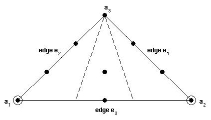
Fig. 7: Element $\mathcal{S}_{4}^{\prime}$.

Next, let $\Lambda_{4}^{T}$ be the interpolation operator associated with $\mathcal{S}_{4}^{\prime}$, and set $\Theta_{4}^{T}:=\Pi^{T}_{4}-\Lambda_{4}^{T}$. Let $r_{1}$ be the basis function of the element $\mathcal{S}_{4}^{\prime}$ that is associated with the degree of freedom $\nabla v(a_{112})(a_{3}-a_{112})$, and let $r_{2}$ be the basis function that is associated with the degree of freedom $\nabla v(a_{122})(a_{3}-a_{122})$. Then for $v\in W^{5,p}(T)$

$$\Theta^{T}_{4}v =\frac{1}{1-(\beta^{(3)})^{2}}\Big{\{}(a_{3}-a_{112})\cdot\big{(}\overline{n}^{(3)}-\tau^{(3)}\beta^{(3)}\big{)}\partial_{\overline{n}^{(3)}}\big{(}v-\Lambda^{T}_{4}v\big{)}(a_{112})r_{1}$$

$$\qquad\qquad+(a_{3}-a_{122})\cdot\big{(}\overline{n}^{(3)}-\tau^{(3)}\beta^{(3)}\big{)}\partial_{\overline{n}^{(3)}}\big{(}v-\Lambda^{T}_{4}v\big{)}(a_{122})r_{2}\Big{\}}.$$

Using the fact $\mathcal{S}_{4}^{\prime}$ is affine equivalent and applying Lemma 3.11 we get

$$1-(\beta^{(3)})^{2}\geq C,\qquad |a_{3}-a_{112}|,\ |a_{3}-a_{122}|\leq Ch_{T},$$

$$|\overline{n}^{(3)}-\tau^{(3)}\beta^{(3)}|\leq 2,\qquad \|v-\Lambda^{T}_{4}v\|_{W^{1,\infty}(T)}\leq Ch_{T}^{4-\frac{2}{p}}\|v\|_{W^{5,p}(T)},$$

$$\|r_{i}\|_{W^{m,q}(T)}\leq Ch_{T}^{-m+\frac{2}{q}},\ i=1,2.\qquad$$

Therefore,

$$\|\Theta_{4}^{T}\|_{W^{m,q}(T)}\leq Ch_{T}^{5-m+\frac{2}{q}-\frac{2}{p}}\|v\|_{W^{5,p}(T)},$$

and consequently,

$$\|v-\Pi_{4}^{T}\|_{W^{m,q}(T)}\leq\|v-\Lambda_{4}^{T}v\|_{W^{m,q}(T)}+\|\Theta^{T}_{4}v\|_{W^{m,q}(T)}\leq Ch_{T}^{5-m+\frac{2}{q}-\frac{2}{p}}\|v\|_{W^{5,p}(T)}.$$

The proof is complete. ∎

We note that if a uniform criss-cross mesh is used such that every triangle has two type I edges (see Figure 2), then $\nabla v(b_{3})(a_{3}-b_{3})=\pm\partial_{\bar{n}}v$ in the definition of $\Sigma^{\prime}_{T}$. This observation leads to the following corollary.

Corollary 3.14.

Suppose $\mathcal{T}_{h}$ is the uniform criss-cross triangulation of $\Omega$, then $S^{h}_{3}=S_{3}^{\prime}$. Hence, $S^{h}_{3}$ is an affine family.

4 Finite element formulation and convergence analysis

Let $V^{h}_{k}\,(k=3,4)$ be the finite element subspaces of $V$ constructed in the previous section. Define

$$V_{k0}^{h}:=\{v\in V^{h}_{k};\ v\big{|}_{\partial\Omega}=\partial_{\bar{n}}v\big{|}_{\partial\Omega}=0\}.$$

Based on the weak formulation (3), we define our finite element method for problem (1)–(2) as seeking $u_{h}\in V_{k0}^{h}$ such that

(19) $$A^{\delta}(u_{h},v_{h})=(f,v_{h})\qquad\forall v_{h}\in V_{k0}^{h}.$$

On noting (5)–(6), an application of Cea’s Lemma [3] yields the following result.

Lemma 2.

There exists a unique solution to (19). Furthermore, the following error estimate holds:

$$\|u-u_{h}\|_{V}\leq C\inf_{v_{h}\in V_{k0}^{h}}\|u-v_{h}\|_{V}.$$

Combining Lemma 2 and Theorem 3.13 with $p=q=2,\ m=1,2$ we immediately get the following energy norm error estimate.

Theorem 4.1.

If $u\in H^{s}(\Omega)\ (s\geq 3)$ then

$$\|u-u_{h}\|_{V}\leq Ch^{\ell-2}\big{(}\sqrt{\delta}+h\big{)}\|u\|_{H^{\ell}},\qquad\ell={\rm min}\{k+1,s\}.$$

Next, using a duality argument, we obtain an error estimate in the $L^{2}$-norm.

Theorem 4.2.

Suppose $u\in H^{s}(\Omega)\ (s\geq 3)$. Then there holds the following error estimate:

(20) $$\|u-u_{h}\|_{L^{2}} \leq C\hat{C}_{0,0}h^{\ell-1}\big{(}\sqrt{\delta}+h\big{)}\|u\|_{H^{\ell}}\qquad\ell={\rm min}\{k+1,s\}.$$

Proof.

Denote the error by $e_{h}:=u-u_{h}$, and let $\varphi\in V_{0}$ be the solution to the following auxiliary problem:

$$A^{\delta}(\varphi,v) =\langle e_{h},v\rangle\qquad\forall v\in V_{0}.$$

It follows from Theorems 2.1 and 2.2 that the above problem has a unique solution $\varphi$ and

(21) $$\sqrt{\delta}\|\nabla\Box\varphi\|_{L^{2}}+\|\Delta\varphi\|_{L^{2}}\leq\hat{C}_{0,0}\|e_{h}\|_{L^{2}}.$$

We then have

(22) $$\|e_{h}\|_{L^{2}}^{2} =A^{\delta}(e_{h},\varphi)=A^{\delta}(e_{h},\varphi-\mathcal{P}_{k}^{h}\varphi)\leq\|e_{h}\|_{V}\|\varphi-\mathcal{P}_{k}^{h}\varphi\|_{V},$$

where $\mathcal{P}_{k}^{h}$ denotes the $L^{2}$-projection to $V^{h}_{k0}$.

By the definition of $\|\cdot\|_{V}$ and (21) we get

(23) $$\|\varphi-\mathcal{P}_{k}^{h}\varphi\|_{V} \leq\sqrt{\delta}\|\Box\varphi-\mathcal{P}_{k}^{h}\Box\varphi\|_{L^{2}}+\|\nabla\varphi-\mathcal{P}_{k}^{h}\nabla\varphi\|_{L^{2}}$$

$$\leq C\sqrt{\delta}h\|\nabla\Box\varphi\|_{L^{2}}+Ch\|\nabla(\nabla\varphi)\|_{L^{2}}$$

$$\leq Ch\bigr{(}\sqrt{\delta}\|\nabla\Box\varphi\|_{L^{2}}+\|\Delta\varphi\|_{L^{2}}\bigr{)}$$

$$\leq C\hat{C}_{0,0}h\|e_{h}\|_{L^{2}}.$$

Thus, it follows from Theorem 4.1, (22), and (23) that

$$\|e_{h}\|_{L^{2}}\leq C\hat{C}_{0,0}h^{\ell-1}(\sqrt{\delta}+h)\|u\|_{H^{\ell}}.$$

The proof is complete. ∎

We conclude this section with a few remarks.

Remark 4.3.

(a) The energy norm error estimate is optimal, on the other hand, the $H^{1}$ and $L^{2}$ norm estimates are optimal provided that $\sqrt{\delta}\simeq h$.

(b) All above convergence results only hold for the restricted meshes, that is, every triangle of the mesh $\mathcal{T}_{h}$ needs to have two type I edges. As already mentioned at the end of Section 3.1, for arbitrary mesh $\mathcal{T}_{h}$, $V^{h}\subset V$ will implies that $V^{h}$ (and $V^{h}_{0}$) needs to be a $C^{1}$ finite element space on $\mathcal{T}_{h}$ such as Argyris, Hsieh-Clough-Tocher, Bogner-Fox-Schmit elements (cf. [3]). In such a case, it follows from Lemma 2 that

$$\|u-u_{h}\|_{V} \leq C\inf_{v_{h}\in V^{h}_{0}}\|u-v_{h}\|_{V}$$

$$\leq C\inf_{v_{h}\in V^{h}_{0}}\bigl{\{}\sqrt{\delta}\|u-v_{h}\|_{H^{2}}+\|u-v_{h}\|_{H^{1}}\bigr{\}}$$

$$\leq Ch^{\ell-2}(\sqrt{\delta}+h)\|u\|_{H^{\ell}},$$

where $\ell={\rm min}\{k+1,s\}$ and $k(\geq 5)$ is the order of the $C^{1}$ finite element. Thus, we still get optimal order error estimate in the energy norm. Although, as expected, using $C^{1}$ finite elements is not efficient to solve the bi-wave problem (cf. [7]).

5 Numerical experiments and rates of convergence

In this section, we provide some numerical experiments to gauge the efficiency and validate the theoretical error bounds for the finite element $S^{h}_{3}$ developed in the previous sections.

Test 1. For this test, we calculate the rate of convergence of $\|u-u_{h}\|$ for fixed $\delta$ in various norms and compare each computed rate with its theoretical estimate. All our computations are done on the square domain $\Omega=(0,1)^{2}$ using the criss-cross mesh. We use the source function

$$f(x,y)= -2048\pi^{4}\delta\big{(}\cos^{2}(4\pi x)-\sin^{2}(4\pi y)\big{)}-32\pi^{2}\Big{\{}\sin^{2}(4\pi y)\big{(}\cos^{2}(4\pi x)-\sin^{2}(4\pi x)\big{)}$$

$$\qquad+\sin^{2}(4\pi x)\big{(}\cos^{2}(4\pi y)-\sin^{2}(4\pi y)\big{)}\Big{\}},$$

so that the exact solution is given by $u(x,y)=\sin^{2}(4\pi x)\sin^{2}(4\pi y)$.

We list the computed errors in Table 1 for $\delta$-values $10,1,10^{-2}$ and $10^{-6}$, and also plot the results in Figure 9. As expected, the rates of convergence depend on both the parameter $h$ and $\delta$. In fact, Corollary 4.1 tells us that for $\sqrt{\delta}>>h$

$$\|u-u_{h}\|_{V} \leq Ch^{2}(\sqrt{\delta}+h)\|u\|_{H^{4}}\leq Ch^{2}\|u\|_{H^{4}},$$

$$\|u-u_{h}\|_{H^{1}} \leq Ch^{2}(\sqrt{\delta}+h)\|u\|_{H^{4}}\leq Ch^{2}\|u\|_{H^{4}},$$

$$\|u-u_{h}\|_{L^{2}} \leq C\hat{C}_{0,0}h^{3}(\sqrt{\delta}+h)\|u\|_{H^{4}}\leq C\hat{C}_{0,0}h^{3}\|u\|_{H^{4}},$$

while for $\sqrt{\delta}\leq h$

$$\|u-u_{h}\|_{V} \leq Ch^{2}(\sqrt{\delta}+h)\|u\|_{H^{4}}\leq Ch^{3}\|u\|_{H^{4}},$$

$$\|u-u_{h}\|_{H^{1}} \leq Ch^{2}(\sqrt{\delta}+h)\|u\|_{H^{4}}\leq Ch^{3}\|u\|_{H^{4}},$$

$$\|u-u_{h}\|_{L^{2}} \leq C\hat{C}_{0,0}h^{3}(\sqrt{\delta}+h)\|u\|_{H^{4}}\leq C\hat{C}_{0,0}h^{4}\|u\|_{H^{4}}.$$

We find that the computed bounds agree with these theoretical bounds.

In addition, although a theoretical proof of the following convergence rate has yet to be shown, the computed solutions also indicate that

$$\|u-u_{h}\|_{2,h} \leq Ch(\sqrt{\delta}+h)\|u\|_{H^{4}},$$

where

$$\|u-u_{h}\|_{2,h}^{2}:=\sum_{T\in\mathcal{T}_{h}}\|u-u_{h}\|_{H^{2}(T)}^{2}.$$

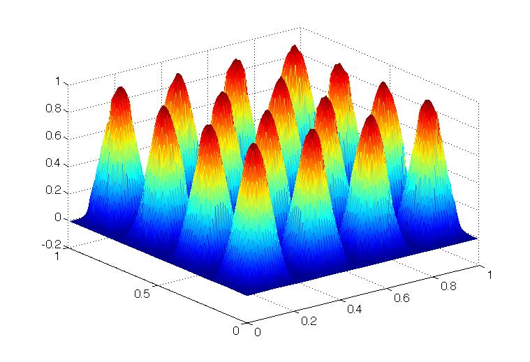
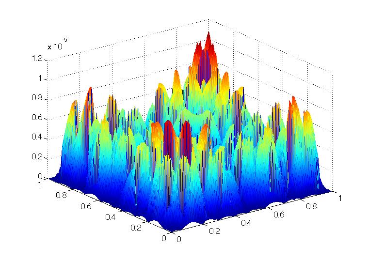
Fig. 8: Test 1. Computed solution (left) and error (right) with $\delta=10^{-2}$ and $h=0.01$.

$\delta$	$h$	$\|\cdot\|_{L^{2}}$ err. (cnv. rate)	$\|\cdot\|_{H^{1}}$ err.(cnv. rate)	$\|\cdot\|_{h,2}$ err. (cnv. rate)	$\|\cdot\|_{V}$ err.(cnv. rate)
10	0.5000	4.17($-$)	26.4($-$)	311.62($-$)	2191.62($-$)
	0.3333	2.76E-01(6.694)	9.54(2.514)	284.05(0.228)	1147.49(1.596)
	0.2000	1.59E-01(1.079)	2.99(2.273)	211.50(0.577)	535.69(1.491)
	0.1000	4.41E-03(5.176)	3.75E-01(2.995)	52.54(2.009)	153.70(1.801)
	0.0500	4.64E-04(3.248)	9.11E-02(2.041)	21.61(1.282)	39.84(1.948)
	0.0400	2.31E-04(3.117)	5.82E-02(2.010)	16.79 (1.130)	25.61(1.980)
	0.0200	2.79E-05(3.054)	1.45E-02(2.004)	8.05(1.060)	6.44(1.992)
	0.0100	3.45E-06(3.014)	3.62E-03(2.001)	3.98(1.016)	1.61(1.998)
	0.0083	1.99E-06(3.006)	2.52E-03(2.000)	3.31(1.006)	1.12(1.999)
	0.0067	1.02E-06(3.004)	1.61E-03(2.000)	2.65(1.004)	0.72(1.999)
1	0.5000	3.93($-$)	25.3($-$)	306.88($-$)	238.43($-$)
	0.2500	2.75E-01(3.837)	9.52(1.413)	283.58(0.114)	123.22(0.952)
	0.2000	1.57E-01(2.523)	2.98(5.210)	210.95(1.326)	56.24(3.515)
	0.1000	4.40E-03(5.152)	3.75E-01(2.989)	52.53(2.006)	15.71(1.840)
	0.0500	4.63E-04(3.249)	9.09E-02(2.043)	21.58(1.284)	4.07(1.950)
	0.0400	2.31E-04(3.118)	5.81E-02(2.012)	16.76(1.132)	2.61(1.981)
	0.0200	2.78E-05(3.055)	1.45E-02(2.005)	8.03(1.061)	0.66(1.992)
	0.0100	3.44E-06(3.015)	3.61E-03(2.001)	3.97(1.016)	0.16(1.998)
	0.0083	1.99E-06(3.006)	2.51E-03(2.000)	3.31(1.006)	0.11(1.999)
	0.0067	1.02E-06(3.004)	1.61E-03(2.000)	2.64(1.004)	0.07(1.999)
	0.0056	5.89E-07(2.999)	1.12E-03(2.000)	2.20(1.003)	0.05(1.998)
$10^{-2}$	0.5000	2.15($-$)	15.4($-$)	276.56($-$)	17.4($-$)
	0.3333	2.25E-01(3.259)	8.38(0.879)	260.32(0.087)	9.48(0.877)
	0.2000	1.02E-01(3.556)	2.53(5.365)	183.36(1.571)	3.07(5.047)
	0.1000	4.21E-03(4.597)	3.69E-01(2.780)	52.08(1.816)	5.22E-01(2.558)
	0.0500	4.36E-04(3.269)	8.55E-02(2.107)	20.31(1.358)	1.25E-01(2.058)
	0.0400	2.15E-04(3.175)	5.38E-02(2.082)	15.52(1.207)	7.93E-02(2.049)
	0.0200	2.50E-05(3.101)	1.30E-02(2.049)	7.21(1.106)	1.94E-02(2.030)
	0.0100	3.06E-06(3.033)	3.21E-03(2.016)	3.53(1.030)	4.82E-03(2.010)
	0.0083	1.77E-06(3.013)	2.23E-03(2.006)	2.94(1.012)	3.35E-03(2.004)
	0.0067	9.02E-07(3.009)	1.42E-03(2.005)	2.34(1.008)	2.14E-03(2.003)
$10^{-6}$	0.5000	3.93($-$)	23.3($-$)	374.18($-$)	23.3($-$)
	0.2500	2.28E-01(4.108)	7.25(1.686)	233.21(0.682)	7.25(1.686)
	0.2000	9.68E-02(3.831)	1.93(5.929)	149.75(1.985)	1.93(5.929)
	0.1000	3.70E-03(4.708)	2.81E-01(2.782)	45.13(1.731)	2.81E-01(2.782)
	0.0500	4.92E-04(2.914)	5.21E-02(2.429)	13.09(1.786)	5.21E-02(2.429)
	0.0400	2.35E-04(3.298)	2.89E-02(2.647)	8.54(1.915)	2.89E-02(2.647)
	0.0200	1.91E-05(3.626)	4.11E-03(2.813)	2.15(1.989)	4.11E-03(2.813)
	0.0100	1.28E-06(3.898)	5.39E-04(2.931)	0.53(2.024)	5.39E-04(2.931)
	0.0083	6.19E-07(3.981)	3.15E-04(2.943)	0.36(2.035)	3.15E-04(2.943)
	0.0067	2.53E-07(4.005)	1.64E-04(2.934)	0.23(2.039)	1.64E-04(2.933)

Table 1: Test 1. Errors with estimated rates of convergence

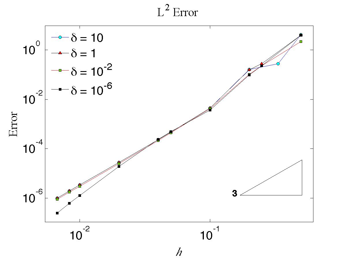
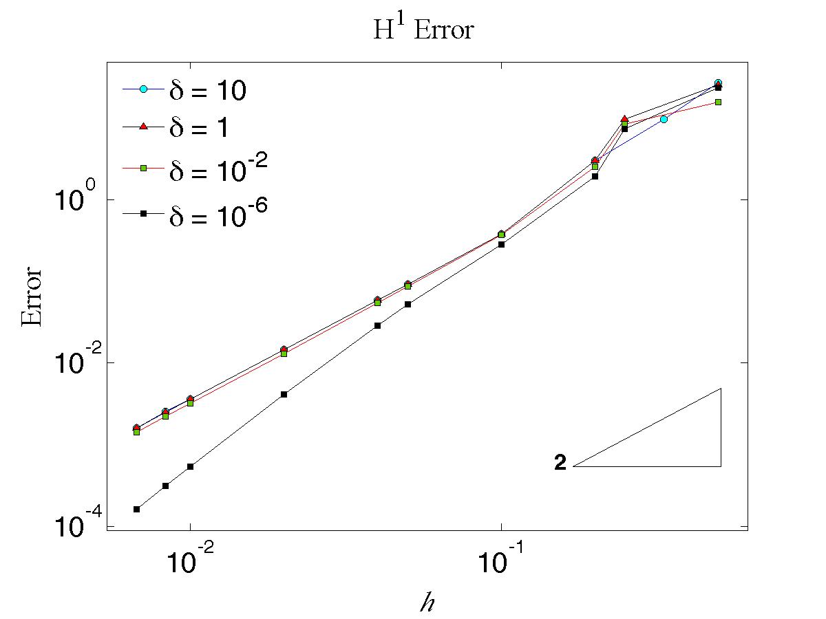
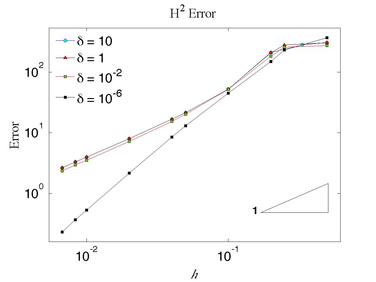
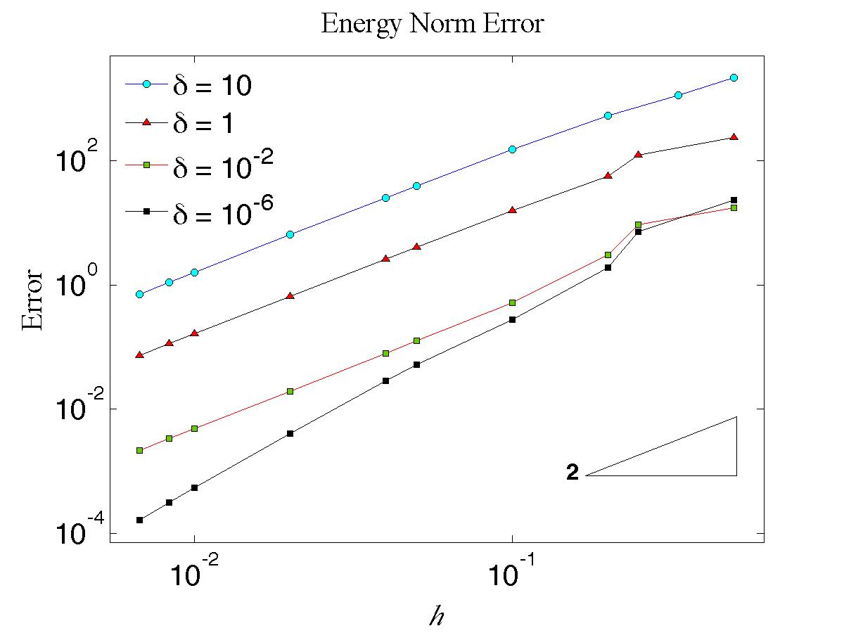
Fig. 9: Test 1. $L^{2}$ norm , $H^{1}$ norm, $H^{2}$ norm, and energy norm errors with $\delta=10,\ 1,\ 10^{-2}$ and $10^{-6}$.

Test 2. This test is the same as the first, but we now use the following source function:

$$f=1.$$

We note that the exact solution is unknown. We plot the solution with $h=0.01$ and $\delta$-values $10,1,10^{-2},$ and $10^{-6}$ in Figure 10. As expected, the solution is more and more like the solution of the corresponding Poisson problem as $\delta$ gets smaller and smaller.

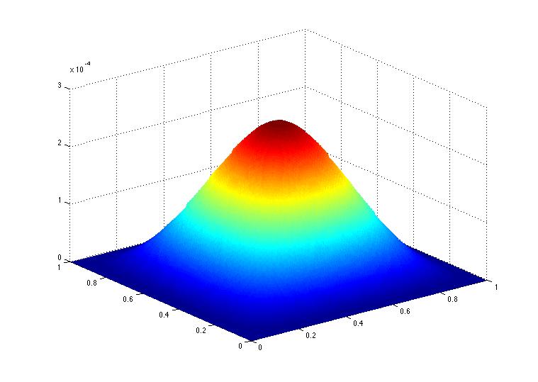
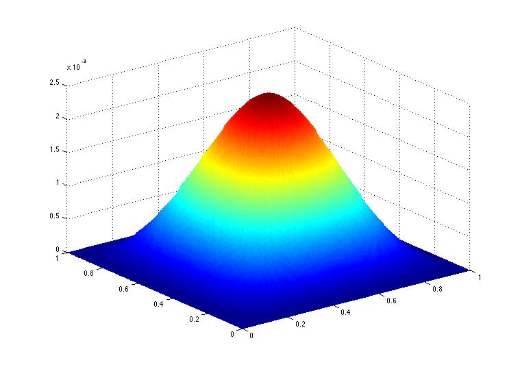
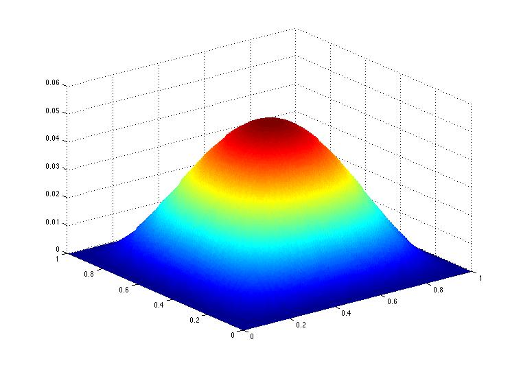
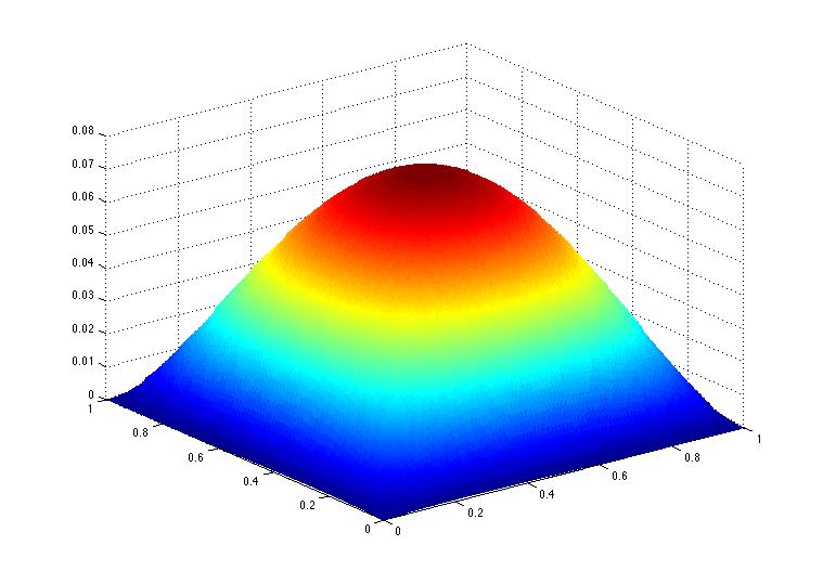
Fig. 10: Test 2. Computed solution with source function $f=1$ and $h=0.01$ with $\delta=10$(top left), $\delta=1$(top right), $\delta=10^{-2}$(bottom left), and $\delta=10^{-6}$(bottom right).

Acknowledgments. The work of both authors was partially supported by the NSF grant DMS-0710831. The authors would like to thank Professor Qiang Du of Penn State University for bringing the bi-wave problem to their attention and for providing the relevant references on $d$-wave superconductors.

References

- [1] D. G. Bourgin and R. Duffin, The Dirichlet problem for the vibrating string equation, Bull. Amer. Math. Soc., 45:851–858, 1939.
- [2] S. C. Brenner and L. R. Scott, The Mathematical Theory of Finite Element Methods, third edition, Springer (2008).
- [3] P. G. Ciarlet, The Finite Element Method for Elliptic Problems, North-Holland, Amsterdam, 1978.
- [4] Q. Du, Studies of Ginzburg-Landau model for d-wave superconductors, SIAM J. Appl. Math, 59(4):1225-1250, 1999.
- [5] L. C. Evans, Partial Differential Equations, AMS, 1998.
- [6] D. L. Feder and C. Kallin, Microscopic derivation of the Ginzburg-Landau equations for a d-wave superconductor, Phys. Rev. B, 55:559–574, 1997.
- [7] X. Feng and M. Neilan, Nonconforming finite element and discontinuous Galerkin methods for a bi-wave equation modeling -wave superconductors, in preparation.
- [8] D. Gilbarg and N. S. Trudinger, Elliptic Partial Differential Equations of Second Order, Classics in Mathematics, Springer, Berlin, 2001. Reprint of the 1998 edition.
- [9] V. L. Ginzburg and L. D. Landau, On the theory of superconductivity, Zh. Èksper. Teoret. Fiz. 20:1064–1082, 1950 (in Russian), in: L.D. Landau, and I.D. ter Haar (Eds.), Man of Physics, Pergamon, Oxford, 1965, pp. 138–167 (in English).
- [10] Y. Ren, J.-H. Xu, and C. S. Ting, Ginzburg-Landau equations for mixed symmetry superconductors, Phys. Rev. B, 53:2249–2252, 1996.
- [11] M. Tinkham, Introduction to Superconductivity, 2rd Edition, Dover Publications, 2004.
- [12] J.-H. Xu, Y. Ren, and C. S. Ting, Ginzburg-Landau equations for a d-wave superconductor with nonmagnetic impurities, Phys. Rev. B, 53(18):12481-12495, 1996.
- [13] A. Ženíšek, Polynomial approximation on tetrahedrons in the finite element method, J. Approxi. Theory, 7:334–351, 1973.
- [14] A. Ženíšek, A general theorem on triangular finite -elements, Rev. Française Automat. Informat. Recherche Opérationnelle Sér. Rouge, 8:119–127, 1974.