Physical signatures of discontinuities of the time-dependent exchange-correlation potential

Abstract

The exact exchange-correlation (XC) potential in time-dependent density-functional theory (TDDFT) is known to develop steps and discontinuities upon change of the particle number in spatially confined regions or isolated subsystems. We demonstrate that the self-interaction corrected adiabatic local-density approximation for the XC potential has this property, using the example of electron loss of a model quantum well system. We then study the influence of the XC potential discontinuity in a real-time simulation of a dissociation process of an asymmetric double quantum well system, and show that it dramatically affects the population of the resulting isolated single quantum wells. This indicates the importance of a proper account of the discontinuities in TDDFT descriptions of ionization, dissociation or charge transfer processes.

I Introduction

The most widely used family of exchange-correlation (XC) functionals in density-functional theory (DFT) hk ; ks ; dft , the local density approximation (LDA) and its gradient-corrected semilocal relatives, has been largely responsible for the enormous popularity of the theory for electronic-structure calculations. Despite many successes, there are important properties of the exact XC potential that are missed by the LDA and many other popular approximations. In this paper, we shall deal with one such property, namely the discontinuity of the XC potential upon change of particle number perdew1982 .

It is well known that the exact XC energy functional must vary linearly as a function of the total number of particles $N$, displaying a derivative discontinuity every time the system passes through an integral value of $N$ perdew ; perdew06 . The delocalization error yang , however, causes the LDA to predict a nonlinear curvature for the change of XC energy with particle number. This has important practical consequences, for instance leading to a description of molecular dissociation where the resulting isolated atoms end up with unphysical fractional electron numbers. Therefore, attempts to model molecular dissociation processes, or any phenomenon that is associated with the transport of charges between well-separated spatial regions or subsystems, must take the discontinuity of the XC functional into account tozer .

In the framework of time-dependent density-functional theory (TDDFT) rg ; book , discontinuities of the time-dependent XC potential upon change of particle number have recently been observed numerically lein ; kummel , and shown to be essential for a proper description of strong-field ionization processes. In such processes featuring rapid electron escape, the formation of steps in the XC potential was observed, which eventually develop into fully-fledged discontinuities. These previous time-dependent studies dealt with one-dimensional model atoms, either putting in the potential discontinuity by hand lein and studying its influence on single versus double ionization probabilities, or calculating the exact XC potential, including steps and discontinuities, by inverting an exact solution of the time-dependent Schrödinger equation kummel .

In this paper we shall work along somewhat different lines: our primary interest is in the question how these features of the time-dependent XC potential influence the behavior of a dissociating system. Rather than carrying out a numerically exact calculation of a simple, few-electron model system, we shall work with physically more realistic (yet still simple) systems, namely doped semiconductor quantum wells in effective-mass approximation, and study the electron loss of single quantum wells, and the dissociation of an asymmetric double quantum well system. In our TDDFT simulations of these processes, we shall compare the adiabatic LDA with and without two types of self-interaction correction (SIC). We will first show that the LDA plus SIC indeed leads to jumps in the XC potential under the appropriate conditions. Then, we will investigate how these jumps affect the dissociation of the double well system.

The paper is organized as follows: Section 2 gives some theoretical background on the concept of self-interaction error and its correction in DFT and TDDFT, as well as the basics of our quantum well model system. In Sections 3 A and B we present results of time-dependent simulations of electron loss and dissociation of single and double quantum wells, respectively. Finally, in Section 4 we give our conclusions.

II Theoretical Background

II.1 Static and dynamic self-interaction correction

In static spin-DFT (SDFT), the noninteracting Kohn-Sham (KS) electrons move in a spin-dependent effective potential given by

$$v_{\sigma}[n]({\bf r})=v_{\rm ext,\sigma}({\bf r})+v_{\rm H}[n]({\bf r})+v_{\rm xc,\sigma}[n_{\uparrow},n_{\downarrow}]({\bf r}).$$ (2.1)

The density is obtained via $n({\bf r})=\sum_{\sigma=\uparrow,\downarrow}n_{\sigma}({\bf r})=\sum_{\sigma=\uparrow,\downarrow}\sum_{k}^{occ}n_{k\sigma}({\bf r})$, where the orbital densities are related to the KS orbitals by $n_{k\sigma}({\bf r})=|\varphi_{k\sigma}({\bf r})|^{2}$. The first term in Eq. (2.1) is the external potential, followed by the Hartree and the XC potential.

One of the exact conditions that the XC potential must satisfy is to be free of the self-interaction error. This means, in particular, that the Hartree and XC potential must cancel each other in a one-electron system. This is automatically true if, for instance, we approximate $v_{\rm xc,\sigma}$ by the exact-exchange (EXX) potential kummel08 . However, for LDA and semilocal functionals this is a hard constraint to be satisfied. Therefore, various procedures for removing the self-interaction error of an approximate XC functional have been developed. Perdew and Zunger pzsic proposed the most widely known SIC for approximate XC energy functionals:

$$E_{\rm xc}^{PZSIC}[n_{\uparrow},n_{\downarrow}]=E_{\rm xc}^{approx}[n_{\uparrow},n_{\downarrow}]-\sum_{\sigma=\uparrow,\downarrow}\sum_{k}^{occ}\left(E_{\rm H}[n_{k\sigma}]+E^{approx}_{\rm xc}[n_{k\sigma},0]\right).$$ (2.2)

For a one-electron system it is immediately seen that the XC contributions cancel each other, and $E_{\rm xc}^{PZSIC}$ becomes equal to the negative of the Hartree energy, thus cancelling $E_{\rm H}$.

The XC potential associated with $E_{\rm xc}^{PZSIC}$, formally defined by

$$v_{\rm xc,\sigma}^{PZSIC}[n_{\uparrow},n_{\downarrow}]({\bf r})=\frac{\delta E_{\rm xc}^{PZSIC}[n_{\uparrow},n_{\downarrow}]}{\delta n_{\sigma}({\bf r})},$$ (2.3)

is not straightforward to obtain by direct variation with respect to the density, since $E_{\rm xc}^{PZSIC}$ is an explicit functional of the orbital densities but only an implicit functional of $n_{\sigma}$ kummel08 . Instead, to obtain a local, state-independent PZSIC XC potential one must apply the so-called optimized-effective potential (OEP) oep methodology or one of its simplifications such as the Krieger-Li-Iafrate (KLI) approach kli . The latter is defined as follows:

$$v_{\rm xc,\sigma}^{KLI}({\bf r})=\frac{1}{2n_{\sigma}({\bf r})}\sum_{k=1}^{occ}|\varphi_{k\sigma}({\bf r})|^{2}\left\{u_{{\rm xc},k\sigma}({\bf r})+\left[\bar{v}_{{\rm xc},k\sigma}^{KLI}-\bar{u}_{{\rm xc},k\sigma}\right]\right\}+\textrm{c.c.},$$ (2.4)

where

$$u_{{\rm xc},k\sigma}({\bf r})=\frac{1}{\varphi_{k\sigma}^{*}({\bf r})}\frac{\delta E_{\rm xc}^{PZSIC}[n_{\uparrow},n_{\downarrow}]}{\delta\varphi_{k\sigma}({\bf r})}$$ (2.5)

and the bars denote orbital averages, e.g. $\bar{v}_{{\rm xc},k\sigma}^{KLI}=\int d^{3}r|\varphi_{k\sigma}({\bf r})|^{2}v_{\rm xc,\sigma}^{KLI}({\bf r})$. Being self-interaction free, the PZSIC formulation also ensures the correct $-1/r$ asymptotic behavior for the XC potential, contrasting with the exponential decay predicted by the LDA. Such a feature is particularly important when dealing, e.g., with the delocalization error yang , since in LDA the outermost electrons are not bound strongly enough. Moreover, it has been shown that the OEP/KLI formalism is able to predict the expected potential discontinuity when the particle number crosses an integer kli .

The PZSIC approach is by no means the only method to get rid of self-interaction errors. A more recent version of SIC, proposed by Lundin and Eriksson lesic1 ; lesic2 , removes the self-interaction directly in the effective potential, which in this approach is given by

$$v_{{\rm xc},k\sigma}^{LESIC}[n_{\sigma},n_{\bar{\sigma}}]({\bf r})=-v_{\rm H}[n_{k\sigma}]({\bf r})+v^{approx}_{\rm xc}[n_{\sigma}-n_{k\sigma},n_{\bar{\sigma}}]({\bf r}),$$ (2.6)

where the XC potential acting on the $k$th orbital depends on all orbital densities except the $k$th. Just like PZSIC, the LESIC approach produces a state-dependent XC potential, which also requires the implementation of the OEP/KLI procedure in order to obtain a local multiplicative KS potential. However, contrary to PZSIC, the LESIC XC approach is formulated directly for the potential, instead of for the energy, so that in principle we cannot use Eq. (2.5) of the OEP/KLI formalism. Nevertheless, one can assume that there exists an energy functional (even though we do not know its structure) which gives rise to the LE orbital potential (2.6), and adopt $u_{{\rm xc},k\sigma}({\bf r})=v_{{\rm xc},k\sigma}^{LESIC}[n_{\sigma},n_{\bar{\sigma}}]({\bf r})$ in Eqs. (2.4) and (2.5). Other features such as the asymptotic behavior and potential discontinuity are also recovered by LESIC, but unlike PZSIC it predicts an erroneous correction even for the hypothetic exact functional perdew05 .

Let us now consider dynamical situations. In TDDFT, the time-dependent analog of Eq. (2.1) is

$$v_{\sigma}[n]({\bf r},t)=v_{\rm ext,\sigma}({\bf r},t)+v_{\rm H}[n]({\bf r},t)+v_{\rm xc,\sigma}[n_{\uparrow},n_{\downarrow}]({\bf r},t),$$ (2.7)

where $n({\bf r},t)=\sum_{\sigma=\uparrow,\downarrow}\sum_{k}^{occ}|\varphi_{k\sigma}({\bf r},t)|^{2}$ follows from the time-dependent KS orbitals. $v_{\rm xc}[n]({\bf r},t)$ is an even more complex object than the static XC potential, since at any given time $t$ it must retain memory effects from all previous times $t^{\prime}\leq t$. Modeling this is a formidable task, and many commonly used TDDFT approaches therefore make use of the adiabatic approximation, which takes an approximate XC potential from static DFT and evaluates it at the instantaneous time-dependent density $n({\bf r},t)$ adiabatic . Accordingly, our previous equations (2.1)-(2.6), dealing with static SIC and KLI calculations, are readily brought under the adiabatic time-dependent umbrella by simply replacing $({\bf r})\rightarrow({\bf r},t)$.

Clearly, adiabatic approximations misrepresent the history of the system, because the resulting TD functional does not have a memory of the past. One way to build memory in the functional has been outlined in reference tdgcm . Here, however, we will focus on aspects where memory effects are not expected to be crucial. Therefore, all time-dependent calculations we present in the following will make use of the adiabatic approach.

II.2 Semiconductor quantum wells

Testing density functionals in a well controlled and modeled environment is of crucial importance for the development of (TD)DFT. In this sense, the quasi two-dimensional electron gases which occur in doped semiconductor heterostructures are useful since they represent an essentially one-dimensional problem: in the effective-mass approximation, only the direction of quantum confinement needs to be analyzed, whereas the lateral or in-plane electronic degrees of freedom can be treated analytically. In particular, GaAs/Al_xGa_1-xAs heterostructures have attracted considerable attention since the effective-mass approximation for conduction band electrons works very well in these systems proetto2 ; proetto ; ullrich .

We assume that such quantum wells have been grown along the $z$ direction and are translationally invariant in the $x-y$ plane. Considering only the conduction band, the KS eigenfunctions can be written as

$$\psi_{q_{\parallel},j\sigma}({\bf r})=\frac{1}{\sqrt{A}}e^{i{\bf q}_{\parallel}\cdot{\bf r}_{\parallel}}\varphi_{j\sigma}(z),$$ (2.8)

where $A$ is an area and $j$ is a subband index, and $\bf r_{||}$ and $\bf q_{||}$ denote in-plane position and wave vectors. The envelope functions $\varphi_{j\sigma}(z)$ satisfy the following one-dimensional KS equation:

$$\left[-\frac{1}{2m^{*}}\frac{d^{2}}{dz^{2}}+v_{\rm ext}(z)+v_{\rm H}[n](z)+v_{\rm xc,\sigma}[n](z)\right]\varphi_{j\sigma}(z)=\varepsilon_{j\sigma}\varphi_{j\sigma}(z)$$ (2.9)

with $n(z)=\sum_{\sigma=\uparrow,\downarrow}n_{\sigma}(z)=\sum_{\sigma=\uparrow,\downarrow}\sum_{j}(\mu-\varepsilon_{j\sigma})|\varphi_{j\sigma}(z)|^{2}/4\pi$, and $\mu$ being the conduction band Fermi level ($\hbar=m=1$ from this point on, so that the effective mass $m^{*}$ is a pure number; further, the bare electric charge $e$ is replaced by an effective charge $e^{*}$). The external potential $v_{\rm ext}(z)$ is prescribed by the design of the quantum well. To describe the dynamics we then propagate the subband envelope functions $\varphi_{j\sigma}(z)$ using the time-dependent KS equation

$$i\frac{\partial}{\partial t}\varphi_{j\sigma}(z,t)=\left[-\frac{1}{2m^{*}}\frac{d^{2}}{dz^{2}}+v_{\rm ext}(z,t)+v_{\rm H}[n](z,t)+v_{\rm xc,\sigma}[n](z,t)\right]\varphi_{j\sigma}(z,t)$$ (2.10)

with the initial condition $\varphi_{j\sigma}(z,t_{0})=\varphi_{j\sigma}(z)$. We use LDA+SIC for $v_{\rm xc,\sigma}[n](z,t)$, and the corresponding TDKLI potential tdkli can be written as

$$v_{\rm xc,\sigma}^{KLI}(z,t)=\frac{1}{2n_{\sigma}(z,t)}\sum_{j=1}^{occ}\frac{(\mu-\varepsilon_{j\sigma})}{4\pi}|\varphi_{j\sigma}(z,t)|^{2}\left\{u_{{\rm xc},j\sigma}(z,t)+\left[\bar{v}_{{\rm xc},j\sigma}^{KLI}(t)-\bar{u}_{{\rm xc},j\sigma}(t)\right]\right\}+\textrm{c.c.}$$ (2.11)

with, e.g., $\bar{v}_{{\rm xc},j\sigma}^{KLI}(t)=\int d^{3}r|\varphi_{j\sigma}(z,t)|^{2}v_{\rm xc,\sigma}^{KLI}(z,t)$. As we will demonstrate below, the TDKLI potential (2.11) retains desirable features of the exact SIC, such as the potential discontinuity each time a new subband $j$ is filled and $-1/z$ asymptotic behavior. In the following, the KS orbitals are propagated on a real-space grid in real time with a Crank-Nicholson algorithm and a time step of 0.05 a.u.

III Results and Discussion

III.1 Barrier suppression of a single well

Mundt and Kümmel kummel showed for a one-dimensional lithium model atom that the time-dependent EXX potential displays humps at its edges as the system loses electrons in an ionization process. In the limit of complete ionization, these humps become more and more steplike, reaching an asymptotic constant value corresponding to the intrinsic derivative discontinuity of the XC potential as the particle number passes through an integer value. Here we study an analogous situation, letting electrons escape from a semiconductor quantum well.

Figure 1: Upper panel: quantum well geometry for studying the effects of barrier suppression. At time $t=0$, the well depth is abruptly reduced to $1/3$ of the initial value. Lower panel: quantum well geometry for studying double-well dissociation. The barrier width grows steadily from 0.2 nm at $t=0$ to 10 nm at $t=250$ a.u.

We consider a $20$nm square GaAs/Al_0.3Ga_0.7As quantum well with conduction band effective mass $m^{*}=0.067$ and charge $e^{*}=e/\sqrt{13}$, and with an electronic density such that the two lowest subbands ($j=1,2$) are occupied. Initially ($t=0$), the difference between the conduction band edges of GaAs and Al_0.3Ga_0.7As is taken as 220meV. Once we have established the KS ground states $\varphi_{j\sigma}(z,t=0)$, for $t>0$ we suppress the barrier height to one third of the initial value. In other words, we consider a sudden switching process which reduces the quantum well depth by 66%, but keeps the square well shape otherwise intact (see upper panel of Fig. 1). Such a process is, of course, highly idealized and would be difficult to realize experimentally. In practice, a static electric field could be used to suppress the quantum well barrier on one side.

Applying an absorbing boundary condition, we then let the system evolve such that the electrons in the second subband are almost completely ionized, and focus our attention on the behavior of the LDA and SIC potentials. We limit ourselves in the following to the exchange-only LDA, $v_{\rm xc,\sigma}^{LDA}[n_{\sigma},n_{\bar{\sigma}}](z,t)=-\left[6/\pi\ n_{\sigma}(z,t)\right]^{1/3}$, applying the TDKLI/PZSIC and TDKLI/LESIC approaches.

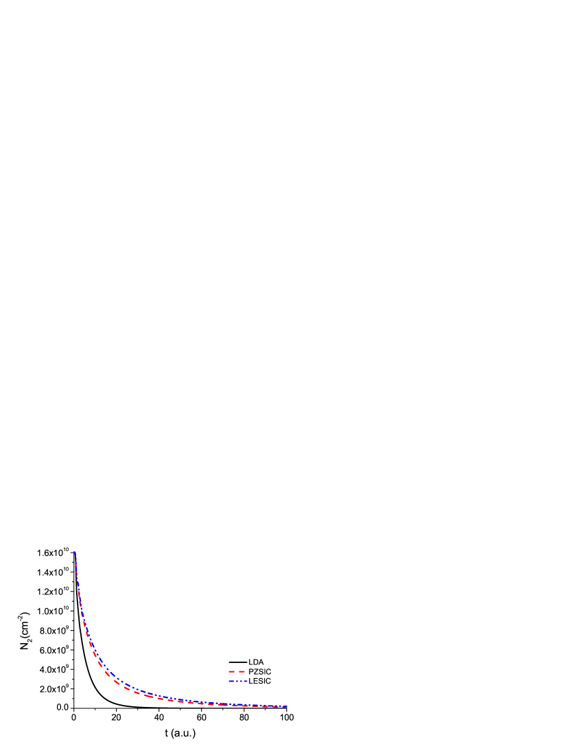
Figure 2: [Color online] Number of electrons in the second subband versus time, illustrating electron escape following a suppression of the quantum well depth to one third of its initial value at $t=0$.

Figure 2 shows the number of electrons per unit area in the second subband, $N_{2}(t)=(2\pi)^{-1}(\mu-\varepsilon_{2\sigma})\int|\varphi_{2\sigma}(z,t)|^{2}dz$, as a function of time. Due to the lowering of the barrier, electrons are able to escape, move away from the quantum well and are absorbed at the boundary, so that the norm of the envelope functions steadily decreases, $\int|\varphi_{2\sigma}(z,t)|^{2}dz<1$. The electrons in the first subband are much more tightly bound, so that the overall ionization of the well is almost exclusively a consequence of emptying the second subband. As one can observe, for pure LDA the ionization occurs much faster than for LDA+PZSIC and LDA+LESIC. This feature is a consequence of the delocalization error yang and the incorrect asymptotic behavior of the LDA: since the electrons are not strongly enough bound to the system, they escape more easily.

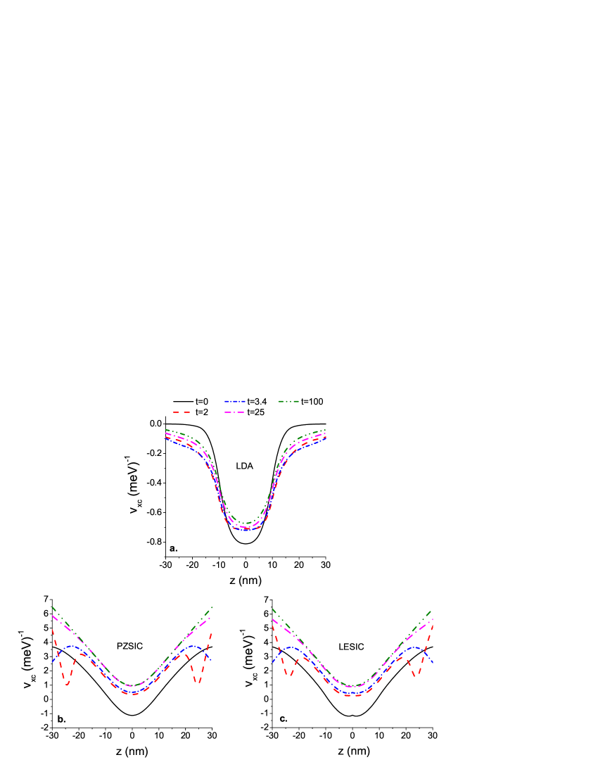
Figure 3: [Color online] Snapshots of the time-dependent LDA, PZSIC and LESIC XC potentials for the electron escape process shown in Figure 2. The ionization of the second subband produces a jump of the XC SIC potentials which builds up via a step structure that moves rapidly away from the well.

Figures 3a, 3b and 3c show snapshots of the XC potentials at different times, in the LDA, PZSIC and LESIC approaches. Starting with two occupied subbands at $t=0$, the second subband is almost completely depleted at $t=100$ and accordingly the XC SIC potentials exhibit a rigid shift between these two situations. As ionization sets in, step structures form and quickly migrate away from the quantum well, along with the escaping electrons. Similar effects were observed previously in the EXX functional for the one-dimensional lithium atom kummel . As expected, the LDA XC potential exhibits neither the formation of the steps nor the resulting jump.

Figure 3 also clearly illustrates the long-range behavior of the LDA and SIC potentials. The LDA exhibits the well-known rapid exponential decay; both SIC potentials have a much longer spatial range, approaching a $-1/z$ behavior in the barrier region, sufficiently far away from the well.

Once the appearance of steps and jumps in the time-dependent XC potential has been confirmed, the next question is whether and how this affects any physical observables. Previous studies kummel were focused mainly on the XC potential itself. In the next section, we present an example where the impact of the discontinuities of the time-dependent XC potential plays an essential role, namely the dissociation process of a double quantum well.

III.2 Dissociation of a double well

A better understanding and more accurate description of dissociation processes is a central issue of much modern research in DFT and TDDFT neepa . Traditionally this problem has been approached from a static point of view perdew . Molecular dissociation displays a basic behavior: the separated atomic systems must have integral charge, and this must be reproduced by any accurate XC functional, either in the static or time-dependent case. Unfortunately, most local and semilocal functionals fail to satisfy this requirement and lead to final dissociation products with fractional charges.

It has been shown perdew ; neepa that, as a molecule dissociates, the XC potential develops a sharp peak at the bond midpoint followed by the buildup of step structures. However, these insights were obtained in a quasistatic picture, using ground-state calculations in some model systems. Here, we use a double quantum well system as a simple time-dependent model of a dissociating heteroatomic molecule. We analyze both the XC potential itself and the effect of jumps or steps on the total number of particles placed in each side of a double well system.

We start at $t=0$ with an asymmetric double quantum well divided by an initially very thin (0.2 nm) barrier, such that electrons can be viewed as sharing both wells, analogous to a molecular orbital. The left well has width 32 nm, and the right one has width 8 nm, and both have the same depth of 220 meV (see lower panel of Fig. 1). The system is populated with a given total number of electrons, $N_{\rm total}=N_{\rm left}+N_{\rm right}$.

For $t>0$, we let the system dissociate, separating the quantum wells from each other by gradually increasing the width of the dividing barrier up to a width of $10$nm. The whole process is allowed to take a total time of 250 a.u., as indicated in the lower panel of Figure 1. We chose such a slow dissociation speed in order to avoid the strong density fluctuations that would be induced if the wells were torn apart too rapidly; nevertheless, the process is far from being adiabatic, and some charge-density oscillations cannot be avoided. At the final separation of 10 nm at $t=250$ a.u., however, these charge-density oscillations have become small ripples, as we will illustrate below. For all practical purposes, the dissociation can then be considered complete.

Figure 4: [Color online] Number of electrons in the left well, $N_{\rm left}$, as a function of total electron number $N_{\rm total}$ of a dissociated double quantum well. Both SIC approaches predict an abrupt decrease of $N_{\rm left}$ approaching the region where the second subband would be filled in the isolated well (dotted lines).

We monitor the total number of particles in the left and right quantum well, $N_{\rm left}$ and $N_{\rm right}$, while the system dissociates. In Figure 4 we display $N_{\rm left}$ as a function of $N_{\rm total}$ when the separation of the two wells is complete at $t=250$ a.u. The horizontal dotted lines indicate the number of electrons $N_{\rm left}$ at which, in a ground-state calculation, the second subband in the isolated left quantum well would start to become occupied. This value of $N_{\rm left}$ is the same for both SIC calculations, but a smaller value is predicted in LDA. The reason for this difference is that SIC (as well as EXX) leads to larger intersubband level spacings due to the different asymptotic behavior of the potential proetto2 (see also Figure 3).

As Figure 4 shows, the LDA predicts a continuous and rather smooth increase of $N_{\rm left}$. By contrast, the SIC results behave dramatically differently when $N_{\rm left}$ approaches the region where the second subband would start to become occupied in the isolated left well. The electrons seem to resist filling the left well, and one even sees a marked decrease of $N_{\rm left}$. If $N_{\rm total}$ continues to increase, $N_{\rm left}$ picks up again, and eventually crosses the threshold of the second subband.

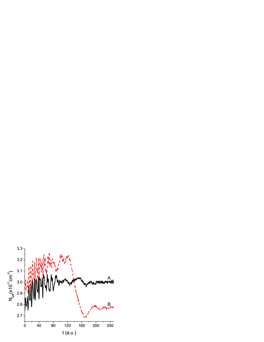
Figure 5: [Color online] Time evolution of $N_{\rm left}$ for the parameters of point A and B indicated in Figure 4. The drop of particle number in the left well occurs as soon as the system is sufficiently separated, so that the subband structure of the isolated left well starts to become relevant.

In order to understand this behavior, we plot in Figure 5 the time evolution of $N_{\rm left}$ calculated with PZSIC, up until the dissociated limit of $10$nm, with parameters corresponding to the points A and B in Figure 4. Situation B starts with a slightly larger density in the left well, but displays a dramatic drop as soon as the two wells are sufficiently separated. The same behavior is found in the LESIC approach, comparing points C and D in Figure 4. This indicates a repulsive force causing electrons to flow from the left to the right well – a clear signature of steps in the potential.

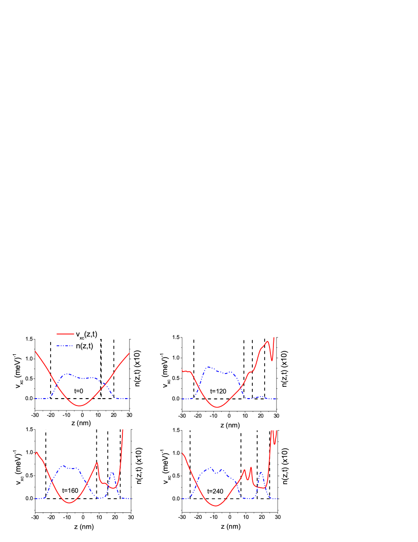
Figure 6: [Color online] Snapshots of the PZSIC XC potential corresponding to curve B in Figure 5. Due to the rise of the XC potential in the the left well relative to the right, electrons are prevented from filling the second subband and are forced to move to the right well instead. A potential peak builds up in region between the wells, leading to a repulsive force. The dashed lines indicate $v_{\rm ext}(z,t)$, and the dash-dotted lines show the density $n(z,t)$.

In Figure 6 we plot snapshots of the PZSIC XC potential and of the density $n(z,t)$ at different times, for parameters corresponding to point B in Figures 4 and 5, i.e., $N_{\rm total}=3.3\times 10^{11}\rm cm^{-2}$ at the initial time. The snapshots of the XC potential clearly illustrate the mechanism preventing the left quantum well from being more filled: Once the double well starts to dissociate, the XC potential builds up steps structures, with a very pronounced sharp peak in the region between the wells. The system resists putting electrons in the second subband: the moment this happens, the potential on the left side shoots up, which means that electrons flow back to the right, as seen from the plots of the density. This effect is clearly absent in the LDA.

It is evident that in a TDDFT computational treatment of molecular dissociation such a behavior of XC potential and density must play a crucial role. The key physical requirement is the neutrality of the isolated atomic system. By building up steps and jumps in the potential, the system avoids incorrect fractional-charge dissociation, forcing electrons to flow from an atom to another. This is the main mechanism which restores the nature of neutral atoms during the dissociation processes, with the correct integral final charges.

IV Conclusion

The results presented here demonstrate that the essential features of the LDA plus SIC approach, namely correct asymptotic behavior and discontinuities upon change of particle number, appear to carry over from static DFT into the time domain. Comparing two different formulations of SIC, PZ and LE, we find only very little difference between them. Our TDDFT calculations were performed in the TDKLI approximation, which leads to an adiabatic XC potential that is state independent. It is known that the TDKLI approach may lead to difficulties with violations of the zero-force theorem mundt , but in our calculations this was not a problem (see also Ref. wijewardane ).

The time-dependent SIC was used in simulating the electron dynamics in doped semiconductor quantum well systems. We first studied electron escape of a single square well upon sudden reduction of the well depth. The main effect of SIC is here due to its asymptotic behavior, which in general makes electron escape proceed at a slower pace compared to the LDA. We observed clear indications of a buildup of a step structure in the XC potential, eventually leading to a discontinuity. These observations are in agreement with what Kümmel and coworkers found earlier for their model atoms lein ; kummel .

The most dramatic effect of the XC potential steps and discontinuities was observed in the simulated dissociation of an asymmetric double quantum well. This system can be compared with a dissociating heteroatomic molecule. Of course, quantum wells are extended systems, so that it is not possible to observe the absolute change in particle number. The corresponding feature in quantum wells is instead the subband population. We found that the dissociation of the double well depends dramatically on the electronic structure of the resulting isolated single wells, namely, whether the second subband in the wider well would be populated or not. It turns out that in SIC the system tends to resist populating the second subband level as long as possible; a pronounced peak structure develops between the two wells, and the depth of the XC potential of the wider well jumps with respect to the potential in the other well. As a result, the total particle numbers of the left and the right well after dissociation are dramatically different from what one would find with the LDA.

Our calculations were carried out for relatively slowly dissociating quantum wells. Nevertheless, we were quite far away from the adiabatic limit, as indicated by the presence of noticeable fluctuations and charge-density oscillations which, however, subsided once the wells were properly separated. The step structures and jumps of the XC potential become more and more difficult to discern the more nonadiabatic and abrupt the dynamics becomes, and tend to be washed out by strong fluctuations of densities and currents.

Further systematic studies to identify dynamical regimes and observables for which the time-dependent XC potential discontinuities are relevant remain an important task. However, there is no doubt that the effect is crucial for generic dissociation or fragmentation processes, and can be captured in TDDFT by simple, self-interaction corrected adiabatic functionals.

Acknowledgment. CAU was supported by NSF Grant No. DMR-0553485 and by Research Corporation. DV and KC were supported by FAPESP and CNPq.

References

- (1) P. Hohenberg and W. Kohn, Phys. Rev., 1964, 136, B864.
- (2) W. Kohn and L.J. Sham, Phys. Rev., 1965, 140, A 1133.
- (3) W. Kohn, Rev. Mod. Phys., 1999, 71, 1253.
- (4) J.P. Perdew, R.G. Parr, M. Levy, and J.L. Balduz, Phys. Rev. Lett., 1982, 49, 1691.
- (5) J.P. Perdew, in Density Functional Methods in Physics, edited by R.M. Dreizler and J. Da Providencia (Plenum, NY, 1985), p.265.
- (6) A. Ruzsinszky, J.P. Perdew, G.I. Csonka, O.A. Vydrov and G.E. Scuseria, J. Chem. Phys, 2007, 126, 104102.
- (7) A.J. Cohen, P. Mori-Sánchez and W. Yang, Science, 2008, 321, 792; P. Mori-Sánchez, A.J. Cohen, and W. Yang, Phys. Rev. Lett., 2008, 100, 146401.
- (8) D. J. Tozer, J. Chem. Phys., 2003, 119, 12697.
- (9) E. Runge and E.K.U. Gross, Phys. Rev. Lett., 1984, 82, 997.
- (10) Time-dependent density functional theory, edited by M. A. L. Marques, C. A. Ullrich, F. Nogueira, A. Rubio, K. Burke, and E. K. U. Gross, Lecture Notes in Physics 706 (Springer, Berlin, 2006).
- (11) M. Lein and S. Kümmel, Phys. Rev. Lett., 2005, 94, 143003.
- (12) M. Mundt and S. Kümmel, Phys. Rev. Lett., 2005, 95, 203004.
- (13) S. Kümmel and L. Kronik, Rev. Mod. Phys., 2008, 80, 3.
- (14) J. P. Perdew and A. Zunger, Phys. Rev. B, 1981, 23, 5048.
- (15) T. Grabo, T. Kreibich, S. Kurth and E.K.U. Gross, in Strong Coulomb Correlations in Electronic Structure Calculations: Beyond the Local Density Approximation, edited by V.I. Anisimov (Gordon and Breach, 2000), p.203.
- (16) J. B. Krieger, Y. Li, and G. J. Iafrate, Phys. Rev. A 45, 101 (1992).
- (17) U. Lundin and O. Eriksson, Int. J. Quantum Chem., 2001, 81, 247.
- (18) P. Novak, J. Kunes, W. E. Pickett, W. Ku and F. R. Wagner, Phys. Rev. B, 2003, 67, 140403.
- (19) J.P. Perdew, A. Ruzsinszky and J. Tao, J. Chem. Phys., 2005, 123, 062201.
- (20) M. Thiele, E.K.U. Gross and S. Kümmel, Phys. Rev. Lett., 2008, 100, 153004.
- (21) E. Orestes, K. Capelle, A. B. F. da Silva and C. A. Ullrich J. Chem. Phys. 2007, 127 124101.
- (22) F.A. Reboredo and C.R. Proetto, Phys. Rev. B, 2003, 67, 115325.
- (23) S. Rigamonti, C.R. Proetto and F.A. Reboredo, Europhys. Lett., 2005, 70, 116; S. Rigamonti and C.R. Proetto, Phys. Rev. Lett., 2007, 98, 066806.
- (24) C.A. Ullrich and G. Vignale, Phys. Rev. B, 1998, 58, 15756.
- (25) C.A. Ullrich, U.J. Gossmann and E.K.U. Gross, Phys. Rev. Lett., 1995, 74, 872.
- (26) D.G. Tempel, T.J. Martínez and N.T. Maitra, arXiv:0812.1247, 2008.
- (27) M. Mundt, S. Kümmel, R. van Leeuwen, and P.-G. Reinhard, Phys. Rev. A., 2007, 75, 050501.
- (28) H. O. Wijewardane and C. A. Ullrich, Phys. Rev. Lett., 2008, 100, 056404.