The opposition effect in the outer Solar System: a comparative study of the phase function morphology

, , , and

Number of pages: 5
Number of tables: 5
Number of figures: 10
Running head: The opposition effect in the outer Solar System

ABSTRACT

In this paper, we characterize the morphology of the disk-integrated phase functions of satellites and rings around the giant planets of our Solar System. We find that the shape of the phase function is accurately represented by a logarithmic model (Bobrov, 1970, in Surfaces and Interiors of Planets and Satellites, Academic, edited by A. Dollfus). For practical purposes, we also parametrize the phase curves by a linear-exponential model (Kaasalainen et al., 2001, Journal of Quantitative Spectroscopy and Radiative Transfer, 70, 529–543) and a simple linear-by-parts model (Lumme and Irvine, 1976, Astronomical Journal, 81, 865–893), which provides three morphological parameters : the amplitude $A$ and the Half-Width at Half-Maximum (HWHM) of the opposition surge, and the slope $S$ of the linear part of the phase function at larger phase angles.
Our analysis demonstrates that all of these morphological parameters are correlated with the single scattering albedos of the surfaces.
By taking more accurately into consideration the finite angular size of the Sun, we find that the Galilean, Saturnian, Uranian and Neptunian satellites have similar HWHMs ($\lesssim$0.5^o), whereas they have a wide range of amplitudes A. The Moon has the largest HWHM ($\thicksim$2^o). We interpret that as a consequence of the ``solar size bias'', via the finite size of the Sun which varies dramatically from the Earth to Neptune. By applying a new method that attempts to morphologically deconvolve the phase function to the solar angular size, we find that icy and young surfaces, with active resurfacing, have the smallest values of A and HWHM, whereas dark objects (and perhaps older surfaces) such as the Moon, Nereid and Saturn's C ring have the largest A and HWHM.
Comparison between multiple objects also shows that Solar System objects belonging to the same planet host have comparable opposition surges. This can be interpreted as a ``planetary environmental effect'' that acts to modify locally the regolith and the surface properties of objects which are in the same environment.

keywords: Planetary rings; Satellites of Jupiter, Saturn, Uranus, Neptune, phase curves; opposition effect, coherent backscattering, shadowing, shadow-hiding, angular size of the solar radius

1 Introduction

The opposition effect is a nonlinear increase of brightness when the phase angle $\alpha$ (the angle between the source of light and the observer as seen from the body) decreases to zero. This effect was seen for the first time in Saturn's rings by Seeliger (1884) and Müller (1885). Now, this photometric effect has been observed on many surfaces in the Solar System : first on satellites of the giant planets, see (Helfenstein et al., 1997) for a review; second on asteroids, (Harris et al., 1989a, b; Belskaya and Shevchenko, 2000) and Kuiper Belt Objects (Belskaya et al., 2008; Rozenbush et al., 2002); and finally on various surfaces on Earth (Verbiscer and Veverka, 1990; Hapke et al., 1996) and for minerals in the laboratory (Shkuratov et al., 1999; Kaasalainen, 2003). The opposition effect on bodies in the Solar System has supplied interesting constraints about the regolith and state of the surfaces (Helfenstein et al., 1997; Mishchenko et al., 2006). Indeed, the opposition effect is now thought to be the combined effect of coherent backscatter (at very small phase angles), which is a constructive interference between grains with sizes near the wavelength of light, and shadow hiding (at larger phase angles), which involves shadows cast by the particles themselves (Helfenstein et al., 1997).
By parametrizing the morphology of the phase functions for $\alpha\thicksim$ 0–20^o, some numerical models have derived physical properties of the medium in terms of regoliths (Mishchenko and Dlugach, 1992a; Shkuratov et al., 1999) and the state of the macroscopic surface (Hapke, 1986, 2002; Shkuratov et al., 1999). However, such characterization of the phase function morphology is restricted by the angular resolution and the phase angle range of the observed phase function. Moreover, some effects (such as the finite size of the Sun and the nature of the soil), which are not yet taken rigorously into account by the most recent models, can play important roles in a comparative study.
For these reasons, it seemed important to test the behavior of the morphology of the phase function before using any physical model.

The use of a simple morphological model is generally not adapted to derive the physical properties of the medium. But for the data set presented here, only the disk-integrated brightness I/F and the phase angle $\alpha$ are available, the corresponding angles of incidence ($i$) and angles of emission ($\epsilon$) are not given for these observations, so we cannot use sophisticated for further investigations analytical models (Hapke, 1986, 2002; Shkuratov et al., 1999) which need the brightness $I/F$ and the three viewing geometry parameters $\alpha$, $\mu$ and $\mu_{0}$ ($\mu$ and $\mu_{0}$ are the cosines of $\epsilon$ and $i$, respectively).
However, the theories developed for the coherent-backscattering and the shadow-hiding effects deduce their properties by parametrizing the opposition phase curve (Mishchenko and Dlugach, 1992a, b; Mishchenko, 1992; Shkuratov et al., 1999; Hapke, 1986, 2002). Thus it is possible to connect the morphological parameters A, HWHM and S with some physical characteristics of the medium derived from these models.

The amplitude A of the opposition peak is generally known to express the effects of the coherent-backscattering. According to Shkuratov et al. (1999); Nelson et al. (2000), A is a function of grain size in such way that A decreases with increasing grain size (we refer to grains as the smallest scale of the surface compared to the wavelenght and virtual entities implied in the coherent backscatter effect, as microscopic roughness). This anti-correlation finds a natural explanation in the fact that for a macroscopic surface, large irregularities with respect to the wavelength create less coherent effects than irregularities with sizes comparable to the wavelength.
Mishchenko and Dlugach (1992b) and Mishchenko (1992) emphasize that A is linked to the intensity of the background $I_{b}$ (defined as a morphological parameter of the linear-exponential function of Kaasalainen et al., 2001), which is a decreasing function of increasing absorption (Lumme et al., 1990); thus A must increase with increasing absorption or decreasing albedo $\varpi_{0}$, which was confirmed by the laboratory measurements of Kaasalainen (2003). Indeed, Kaasalainen (2003) remarked that the opposition surge increases and sharpens when irregularities are small and that the opposition surge decreases with increasing sample albedo.

The half width at half maximum HWHM, is also associated to the coherent-backscatter effect. It has been related to the grain size, index of refraction, and packing density of regolith, by previous numerical studies (Mishchenko, 1992; Mishchenko and Dlugach, 1992a; Hapke, 2002). The variation of HWHM with these three physical parameters is complex; see Fig. 9 of (Mishchenko, 1993): HWHM reached its maximum for an effective grain size near $\lambda$/2 and increases when the regolith grains' filling factor $f$ increases. For high values of $f$, the maximum of HWHM occurs for a larger grain size.
However, several studies Helfenstein et al. (1997); Nelson et al. (2000); Hapke (2002) defined two HWHM parameters : for the Hapke (2002) model, the coherent-backscatter HWHM ($h_{c}$), which is defined similarly to that in the model of Mishchenko (1992), and the shadow hiding parameter $h_{s}$. Applying this model to Saturn's rings, French et al. (2007) found that the coherent-backscatter peak is about ten times narrower than the shadow-hiding peak, but neither $h_{c}$ nore $h_{s}$ equals to the morphological width of the peak HWHM. This reinforces the idea that a coupling of the two opposition effect mechanisms at small phase angles could be responsible for the observed surge width.

Since the efficient regime of the shadow hiding is 10^o–40^o(Buratti and Veverka, 1985; Helfenstein et al., 1997; Stankevich et al., 1999) and that of the coeherent bakscattering does not exceed several degrees (Helfenstein et al., 1997), the slope of the linear part $S$ can be regarded as the only parameter that mirrors the shadow hiding solely. This slope depends on the particle filling factor D, which relates to the porosity of the regolith of a satellite and the ratio between the particle size and the physical thickness of the ring for a planetary ring (Irvine, 1966; Stankevich et al., 1999; Kawata and Irvine, 1974). For a satellite, by ``particles'' we mean the macroscopic scales of the surface, which are implied in the shadow hiding effect.
In the shadowing model of Irvine (1966) and Kawata and Irvine (1974) (which consists of the effects of shadows for a monolayer of particles), when the slope is shallow, the variation of $\alpha$ does not change the visibility of shadows and the particle filling factor must be high to make the proportion of shadows small for any observation geometry. By contrast, when S is steep, the particle filling factor is smaller and will contribute to a broad and large peak with a weak amplitude which will be regarded as a slope.
In the shadow hiding model (i.e., multilayer shadowing), the larger the optical depth and the volume density D, the steeper the phase function is at large phase angles (10^o–40^o, Stankevich et al., 1999). However, at larger phase angles, the behavior of the absolute slope with albedo could change according to a more efficient regime of the shadow hiding (50^o–90^o, Stankevich 2008, private communication).

For a compact medium such as a satellite's surface, the slope at very large angles ($\alpha$>90^o) is a consequence of topographic roughness, the so-called roughness parameter $\theta$ in the Hapke (1984, 1986) model. Then a steeper slope is due to a surface tilt which varies from millimeter to centimeter scales (Hapke, 1984). However, the roughness can influence the phase curve at smaller phase angles as underlined by Buratti and Veverka (1985), also according to the laboratory measurements of Kaasalainen (2003), the slope of the phase function ($\alpha$<40^o) increases with increasing roughness. From the theoretical assertions made above, the HWHM and the amplitude are governed by both coherent backscatter and shadow hiding effects, whereas the slope of the linear part of the phase curve is mirrors the unique expression of the shadow hiding effect.

The goal of this paper is to understand the role played by the two known opposition effects (coherent backscatter and shadow hiding) on the morphology of the surge for different surface materials, which have different values of grain size, regolith grain filling factor, absorption factor (or inverse albedo), particle filling factor and vertical extension, by making some comparisons with the three morphological output parameters A, HWHM and $S$.

This paper describes the results of a full morphological parametrization and comparison of phase functions of the main satellites and rings of the Solar System in order to compare the influence of parameters not yet implemented in actual models and simulations. Section 2 describes the data set that we used here and the specific reduction we added to these previously published data in order to compare them more easily. We also present the morphological models that have supplied the parameters and discuss their link with physical properties of the surfaces. In Section 3, we focus on the specific behaviors of the morphological parameters, as a function of the single-scattering albedo, the distance from the Sun and the distance from the center of the parent planet. Section 4 is dedicated to a discussion in which we physically interpret the general behaviors obtained with a deconvolution method. Conclusions and future work that would be of interest are drawn in Sections 5.

2 Data set description and reduction

2.1 The opposition effect around a selection of rings and satellites of the giant planets

We have applied a fitting procedure to a set of phase curves of satellites and rings obtained by previous ground-based and in situ optical observations (see Table 1 for references). The spectral resolution of the filters used for these observations are not rigorously mentionned by theirs authors, and because we mix for some objects phase curves of close wavelength, we give an approximate value of the wavelength of observation (the uncertainty of the approximated values is roughly 100 to 200 nanometers).
For a comprehensive study of the morphology of the opposition phase curves, the solar phase curves of the Galilean satellites (Io, Europa, Ganymede and Callisto) and the jovian main ring were chosen, as well as the phase curves of the Saturnian rings (the classical A, B, and C rings and the tenuous E ring) and some Saturnian satellites (Enceladus, Rhea, Iapetus and Phoebe); the rings and satellites of Uranus [We refer to the seven innermost satellites of Uranus – Bianca, Cressida, Desdemona, Juliet, Portia, Rosalind and Belinda – as the Portia group, to follow the designation of Karkoschka (2001). The phase function of the Portia group is then the averaged phase function for these seven satellites.], including the Portia group and three other Uranian satellites, Titania, Oberon and Miranda; and finally two Neptunian ring arcs (Egalité and Fraternité) and two satellites of Neptune (Nereid and Triton). For all the satellites of this study, the phase function is representative of the leading side because they have, in general, better coverage at small phase angles (except for Iapetus which have a trailing side brighter, we then use the Iapetus' trailing side data). References for the phase curves that we use in this study are given in table 1.

Insert Table 1

This study should give an extensive comparison between rings around the giant planets (Jupiter, Saturn, Uranus and Neptune), as well as a comparison between rings and satellites for each giant planet of our Solar System. For practical purposes, the well-known phase curve of the Moon is added as a reference.

2.2 Data set reduction

In order to properly compare the morphological parameters of the objects whose phase curves are given as magnitudes, we have converted the magnitude $M$ to the disk-integrated brighness $I/F$ by using :

$$I/F=10^{-0.4M}$$ (1)

(Domingue et al., 1995). This modification allows us to directly compare the slope of the linear part of all the curves in the same unit.

2.3 Data set fits: the morphological models

The purpose of the present paper is to provide an accurate description of the morphological behavior of the observed phase curves. This is the very first step prior to any attempt to perform either analytical or numerical modeling. As a consequence, special care has been given here to parametrizing the observations efficiently and conveniently. In addition, morphological parametrization is necessary to efficiently compare numerous phase curves and derive statistical behavior, as will be done in Section 3.
Several morphological models have been used in the past to quantitatively describe the shape of the phase functions : the logarithmic model of Bobrov (1970), the linear-by-parts model of Lumme and Irvine (1976) and the linear-exponential model of Kaasalainen et al. (2001). The specific properties of these three models make them adapted for different and complementary purposes. The logarithmic model is an appropriate and simple representation of the data, the linear-by-parts model is convenient to describe the shape in an intuitive way, and finally the linear-exponential model is commonly used for the phase curves of Solar System bodies (see the comparative study of Kaasalainen et al., 2001).

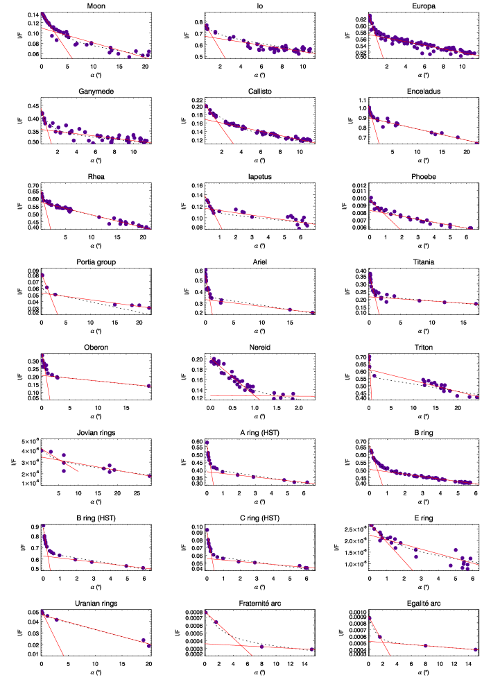
Figure 1: Phase curves of a selection of rings and satellites in the Solar System (see Table 1 for references). The solid curves correspond to the best fit obtained with the linear-by-parts model and the dotted curves to the best linear-exponential fit.

Insert Fig. 1

2.3.1 The linear-by-parts model

For an intuitive description of the main features of the phase curves, the linear-by-parts model is the most convenient one. It is constituted of two linear functions fitting both the surge at small phase angles ($\alpha<\alpha_{1}$) and the linear regime at larger phase angles ($\alpha>\alpha_{2}$), where, generally, $\alpha_{1}\neq\alpha_{2}$. Besides $\alpha_{1}$ and $\alpha_{2}$, this function depends on 4 parameters, $A_{0}$, $B_{0}$, $A_{1}$, and $B_{1}$, such that:

$$I/F(\alpha<\alpha_{1})=-A_{0}\cdot\alpha+B_{0}$$ (2)

$$I/F(\alpha>\alpha_{2})=-A_{1}\cdot\alpha+B_{1}$$ (3)

Lumme and Irvine (1976) and Esposito et al. (1979) use $\alpha_{1}$=0.27^o and $\alpha_{2}$=1.5^o. By testing several values of $\alpha_{1}$, it appears that for our data set, values of $\alpha_{1}=0.5$^o and $\alpha_{2}$=2^o provide the best results, so these values are now adopted in the rest of the paper except for the Moon and tenuous rings for which we take $\alpha_{1}=1$^o.
In terms of the four parameters $A_{0}$, $B_{0}$, $A_{1}$, and $B_{1}$, the shape of the curve is characterized by introducing three morphological parameters : A, HWHM and S designating the amplitude of the surge, the half-width at half-maximum of the surge, and the absolute slope at ``large'' phase angles (i.e., a few degrees up to tens of degrees), respectively. The parameters are defined by :

$$\textrm{A}=\frac{B_{0}}{B_{1}}~{}~{}~{}~{}~{}~{}~{}~{}\textrm{HWHM}=\frac{(B_{0}-B_{1})}{2(A_{0}-A_{1})}~{}~{}~{}~{}\textrm{and}~{}~{}~{}~{}S=A_{1}$$ (4)

Even if all the part of the opposition curve cannot be fitted by two linear functions, this model offer a convenient description of the main trends of the phase curve.

2.3.2 The linear-exponential model

The linear-exponential model describes the shape of the phase function as a combination of an exponential peak and a linear part. Its main interest is that it has been used in previous work for the study of the backscattering part of the phase curves of the Solar System's icy satellites and rings (Kaasalainen et al., 2001; Poulet et al., 2002).
However, as noted by French et al. (2007), we find that this model does not fit the phase curves well: in particular A, HWHM and S are under- or overestimated. In addition, the converging solutions found by a downhill simplex technique have large error bars, which means that a large set of solutions is possible and thus produce some difficulties for the comparison with the other objects.
For completeness, we give the four parameters of this model : the intensity of the peak $I_{p}$, the intensity of the background $I_{b}$, the slope of the linear part $I_{s}$ and the angular width of the peak $w$ such that the phase function is represented by :

$$I/F=I_{b}+I_{s}\cdot\alpha+I_{p}\cdot e^{-\frac{\alpha}{2w}}$$ (5)

As $\alpha\rightarrow 0$, $\exp({-\alpha/2w})\rightarrow 1-\alpha/2w+\mathcal{O}$($\alpha^{2}$), so that the slope approaches $I_{s}+I_{p}/(2w)$. The degeneracy of these parameters may explain some of the difficulty in obtaining good fits described above. For consistency with previous work, we can express the amplitude and HWHM of the opposition surge in this model as:

$$\textrm{A}=\frac{I_{p}+I_{b}}{I_{b}}~{}~{}~{}~{}~{}~{}~{}~{}\textrm{HWHM}=2\cdot\ln 2w~{}~{}~{}~{}\textrm{and}~{}~{}~{}~{}S=-I_{s}$$ (6)

We report in Table 2, the morphological parameters of the linear-by-parts model and that of the linear-exponential model.

Insert Table 2

2.3.3 The logarithmic model

As noted by Bobrov (1970), Lumme and Irvine (1976) and Esposito et al. (1979), we remark that a logarithmic model describes the phase curves very well. It depends on two parameters ($a_{0}$ and $a_{1}$). This model has the following form :

$$I/F=a_{0}+a_{1}\cdot\ln(\alpha)$$ (7)

In general, this model is the best morphological fit to the data. However, $a_{0}$ and $a_{1}$ are not easily expressed in terms of A, HWHM and S, since the model's dependence on $\alpha$ is scale-free. Thus we report the values of these two parameters in table 3 to allow an easier reproduction of the observational data.

2.3.4 A method that takes into account the angular size of the Sun

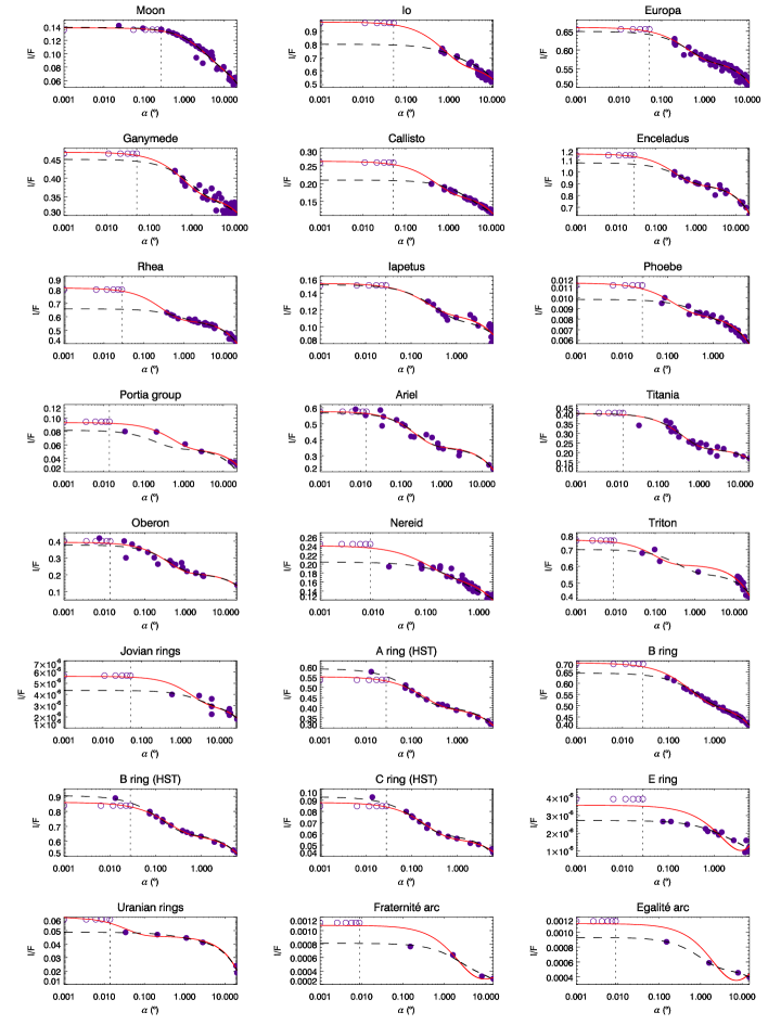
Figure 2: Phase curves of a selection of rings and satellites in the Solar System. The solid curves correspond to the best fit obtained with the linear-exponential model convolved with the size of the Sun (using extrapolated data below the angular size of the Sun, empty symbols) and the dashed curves correspond to the best linear-exponential fit (using only original data, filled symbols). The vertical dotted lines represent the angular size of the Sun at the observation time (see Table 6 of Appendix).

For all the phase curves presented here, a comparison of their surges could be compromised because they have different values of their observed minimum phase angle values. For example, data for the Galilean satellites never reach 0.1^o, whereas data for Saturn's rings almost reach 0.01^o.
Although the behavior within the angular radius of the Sun represents a small part of the phase function, these smallest phase angles are crucial to constrain the fit, especially for the linear-exponential model. Indeed, when $\alpha\rightarrow 0$, the linear-exponential function tends toward $I_{b}+I_{p}/(2w)$; as a consequence, this function flattens at very small phase angles.
However, in some cases this flattening does not correspond to the expected flattening due to the angular size of the Sun because the linear-exponential flattening fits itself arbitrarily with the phase angle coverage. The less points there are at small phase angles, the sooner will occur the flattening of the phase function.
Déau et al. (2008) showed for Saturn's rings that the behavior of the surge was accurately represented by a logarithmic model between 15^o and 0.029^o, where 0.029^o corresponds to the angular size of the Sun at the time of the Cassini observations. Below 0.029^o, the resulting phase function flattens, whereas the logarithmic function continues increasing. The use of this fact observed specifically for Saturn's rings and its generalization to the Solar System objects of this study allows us to create extrapolated data points. Indeed, it is more convenient to use extrapolated data points than convolve the linear-exponential function or the logarithmic function with the solar limb darkening. First because, for incomplete phase functions, the flattening of linear-exponential function is almost uncontrollable and second because for the logarithmic model, even if a convolution is possible, linking the morphological parameters A, HWHM and S to the outputs $a_{0}$ and $a_{1}$ is not trivial.
The method to create extrapolated data points consists of first fitting the logarithmic model to the data and then taking the value of the logarithmic function at the phase angle which corresponds to the solar angular size ($\alpha_{\odot}$, see Appendix). We then give to six points the same $y$-value : I/F($\alpha=\alpha_{\odot}$) and $x$-values ranging from 0.001^o to $\alpha_{\odot}$ of phase angle. These extrapolated data points are represented in Figure 2 (the full method is detailed in the Appendix). The extrapolated data and the original data are then fitted by the linear-exponential model in the last step.

Insert Fig. 2

For the Moon, Ariel and Oberon, for which the phase curve has a few points below the solar angular radius, we can see that the extrapolated points match the observational points quite well. This proves that the solar angular size effect is a flattening of the phase function below $\alpha_{\odot}$. In the case of the HST data for Saturn's rings, for which we have also a few points below the solar angular radius, the extrapolated points are a bit smaller than the observed points. This is may be due to the fact that the data of French et al. (2007) are already deconvolved by another method.

We also performed a convolution of the linear-exponential function to a limb darkening function (see Appendix), but this refinement did not significantly change the values of A, HWHM and S, because the linear-exponential model already flattens as $\alpha\rightarrow 0$. Thus, by adding extrapolated data below $\alpha_{\odot}$, we are sure that the resulting fitting function will have a constant behavior below $\alpha_{\odot}$ and that the resulting fitting function will take into account the angular size of the Sun. However, we assume that all bodies have a logarithmic increase up to the solar angular radius, which is only confirmed for Saturn's rings. Output parameters of our best fit for the ``extrapolated linear-exponential'' function are given in table 3.

Insert Table 3

2.3.5 A method of solar size deconvolution

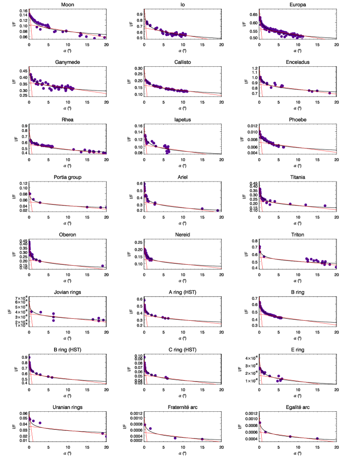
Figure 3: Phase curves of a selection of rings and satellites in the Solar System. The solid lines correspond to the best fit obtained with the linear-by-parts fit to the logarithmic model (in solid curves).

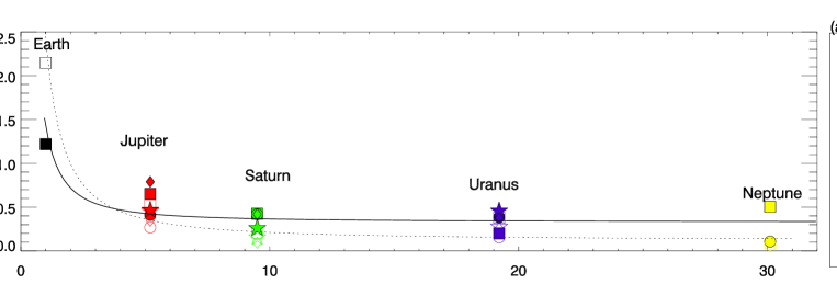
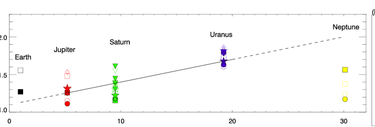
Figure 8: Variation of the morphological parameters HWHM and A derived with the linear-by-parts model (filled symbols and solid line) and the extrapolated linear-exponential model (empty symbols and dotted line) with respect to the distance from the Sun (distances are taken from Murray and Dermott, 2000).

Although the behavior at phase angles smaller than the solar angular radius represents a small part of the surge, a comparison of the surge of Solar System rings and satellites could be compromised because they have different values for the mean solar angular radius ($\alpha_{\textrm{min}}$=0.051, 0.028, 0.014, 0.009^o respectively for Jupiter, Saturn, Uranus and Neptune at their mean distances from the Sun). Indeed, according to the results presented here, the amplitude and HWHM seems linked to the finite angular size of the Sun. However, our morphological study doesn't clearly show that the Sun's angular size effect is preponderant for the amplitude A, because even considering more accurately the ``solar environmental effect,'' the surges of Neptune's satellites have smaller amplitudes than those of Uranus (figure 8b). This contradicts the theoretical assumption that the solar angular size would give the largest amplitude to the most distant objects, for which the Sun has the smallest angular size. Because we previously noted that the effect of the ``solar environmental effect'' was to flatten the phase function when the phase angle is less than or equal to the solar angular radius (Déau et al., 2008), a naive deconvolution method would be to allow the phase curve to rise below $\alpha_{\odot}$. This is also suggested by a previous deconvolution of HST data on Saturn's rings, for which the brightness still increases below $\alpha_{\odot}$ (French et al., 2007). However, the linear-exponential function is not appropriate for this purpose because it intrinsically flattens as $\alpha\rightarrow 0$. Thus the only morphological function that allows an increase, even at very small phase angles, is the logarithmic function. In particular, this function allows the same increase of the brightness above and below the solar angular radius (without break in the brightness), then using this function simulates a point source of light. However, we assume that the smallest phase angles are about $\alpha$=0.001^o, in this way, if a physical flattening should be performed by the coherent backscattering or the shadow hiding effect, it will be possible at these phase angles.
The logarithmic function fits the phase function quite well at small and large phase angles (0.1-15^o, Déau et al., 2008); however, none of the morphological parameters A, HWHM and S are well-defined in this model. Because the logarithmic model is a good representation of the data and perform a kind of deconvolution at phase angles less than $\alpha_{\odot}$, we fit this function by the linear-by-parts function. As shown in figure 3, the fitting results of this crude deconvolution method is reasonably acceptable when the phase function is plotted on a linear scale of phase angle.

Insert Fig. 3

However, on a logarithmic scale of $\alpha$, the linear-by-parts fit is obviously not acceptable because intrinsically, a linear function cannot fit a logarithmic increase. As a consequence, we have slightly changed the linear-by-parts parameters in order to take into account the inappropriate flattening of this function, compared to the logarithmic function. Because the y-intercept $B_{0}$ of the linear-by-parts model is less than the values of the logarithmic function when $\alpha$<0.01^o, we replace $B_{0}$ by the value of the logarithmic function when $\alpha$=0.001^o :

$$B_{0}^{\prime}=a_{0}+a_{1}\cdot\ln(10^{-3}),$$ (8)

where $a_{1}\leq 0$, in such a way that the amplitude and the angular width are now given by :

$$A=\frac{B_{0}^{\prime}}{B_{1}}~{}~{}~{}~{}~{}~{}~{}~{}\textrm{and}~{}~{}~{}~{}~{}~{}~{}~{}\textrm{HWHM}=\frac{(B_{0}^{\prime}-B_{1})}{2(|a_{1}|-A_{1})}$$ (9)

where $|a_{1}|$ is the absolute slope of the logarithmic function (see section 2.3.3). Replacing $|a_{1}|$ by $A_{0}$ in the formula for HWHM was motivated by the fact that the original values of the linear-by-parts parameters were systematically the same (HWHM$\thicksim$0.22^o for $\alpha_{1}$=0.3^o). This is due to the fact that the logarithmic function is a fractal function, so it is not possible to obtain a Half-Width at Half Maximum. Values of the linear-by-parts parameters A, HWHM and S are given in Table 5. Our best result is probably that for the B ring, for which we previously found different values of A from the Franklin and Cook (1965) data and the French et al. (2007) data (A=1.30 and A=1.38 respectively, see table 2 with the convolved models). The discrepancy was still present with the extrapolated linear-exponential model (A=1.35 for Franklin and Cook (1965) and A=1.32 for French et al. (2007)), due to the fact that the solar angular size was different at the two observation times (see table Appendix6). Now, with the unconvolved model, the discrepancy of the two values is somewhat reduced compared to values from the fit to the original data : A=1.82 for Franklin and Cook (1965) and A=1.77 for French et al. (2007), table 5, which implies that the angular size effect is now absent.

Insert Table 5

3 Results

Our procedure is to interpret more carefully the morphological results of a large dataset. We start first by studying the behaviors of the morphological parameters with the single scattering albedo with the raw data (Section 3.1 and 3.2) and the improved data that take into account of the solar size of the Sun (Section 3.3). In a last step, we freed from the solar size biais by trying to look the opposition effect in the outer Solar System with the same solar size, assumed to be a point (Section 3.4).

3.1 Behaviors of the morphological parameters

In this section we compare the morphological parameters as a function of the single scattering albedo $\varpi_{0}$.
Since the single scattering albedo $\varpi_{0}$ represents the ratio of scattering efficiency to total light extinction over the phase angle range (Chandrasekhar, 1960), its value must be computed with the largest coverage of phase angle as possible (0 to 180 degrees). This is why we did not compute the single scattering albedo with the phase curves presented in this paper but we use previously published values of single scattering albedo computed from phase curves with a larger phase angle coverage than ours and a wavelength close to ours. Thus, references for phase curves (table 1) and references for $\varpi_{0}$ (table 4) are not always the same.

Insert Table 4

We did not found single scattering albedo values for the jovian main ring and the Saturn's E ring, so these two objects will be excluded of the study of the mophological parameters with the single scatterig albedo.

3.1.1 Variation of the angular width of the surge with albedo

First, we discuss the variation of HWHM=$f(\varpi_{0})$ derived from the linear-by-parts model (Figure 4a) and HWHM=$f(\varpi_{0})$ derived from the extrapolated linear-exponential model (Figure 4b). Interestingly, the variation differs according to the morphological model : the first case leads to a decrease of HWHM when $\varpi_{0}$ increases, while the latter case leads to an increase of HWHM when $\varpi_{0}$ increases.

Insert Fig. 4

The different results for HWHM=$f(\varpi_{0})$ between the linear-by-parts results (well fitted by HWHM$\thicksim 0.9\times 0.3^{\varpi_{0}}$, Figure 4a) and the extrapolated linear-exponential results (represented by HWHM$\thicksim 0.15+0.19\varpi_{0}$, Figure 4b) is mainly due to the points which correspond to the Moon, Callisto and Nereid. Indeed, in general, values from the extrapolated linear-exponential model significantly decrease for the outer Solar System objects, whereas the value for the Moon increases by almost 1^o. This is due to the fact that when we take into account the Sun's angular size, this effect lower the values of HWHM for the incomplete phase functions.
However, Figure 4 shows a large dispersion of HWHM with albedo.

3.1.2 Variation of the amplitude of the surge with albedo

Figure 5 shows a weak dependence of the amplitude of the surge on the albedo for the satellites, already noted by Helfenstein et al. (1997); Rozenbush et al. (2002).

Insert Fig. 5

In both cases (linear-by-parts model, Figure 5a and extrapolated linear-exponential model, Figure 5b) we note a dependence of $A$ with $\varpi_{0}$, which follow a function leading to a decrease of $A$ when $\varpi_{0}$ increases (A$\thicksim 1.65\times 0.72^{\varpi_{0}}$ in Figure 5a and A$\thicksim 1.75\times 0.72^{\varpi_{0}}$ in Figure 5b). The consistent trends in both cases imply that the finite size of the Sun was correctly derived by the linear-by-parts model.
The decrease of $A$ with increasing $\varpi_{0}$ could be understood by a relation between the amplitude and the single scattering albedo via the intensity of the background phase function $I_{b}$ (with the linear-exponential model), which is inversely proportional to the albedo. Thus, the predicted trend of Lumme et al. (1990) is confirmed by our present results.
In addition, Figure 5b labels satellites by color to indicate their parent planet. This figure indicates that distant objects (such as the Uranian satellites) have a significantly larger amplitude than less distant objects (such as the Galilean or Saturnian satellites) while the Neptunian satellites have values in the average. Then it must be considered that the finite size of the Sun has a role in the amplitude's value (Shkuratov, 1991). As a consequence, even if the trend of A=$f(\varpi_{0})$ is well explained by theoretical considerations, one can remark that the large dispersion in this correlation could be due to other effects (such as the finite size of the Sun) that weakens the albedo dependence of A. Thus, as for HWHM, we cannot physically interpret the variation of HWHM and A as long as they are convolved with the effect of the solar angular size.

3.1.3 Variation of the slope of the linear part with albedo

The last morphological parameter is the slope S, which we represent as a function of the single scattering albedo $\varpi_{0}$ for the rings (Figure 6a) and satellites (Figure 6b) of the Solar System.

Insert Fig. 6

In this figure, rings and satellites have different values of slope as function of their albedo, and a slight increase for S with increasing $\varpi_{0}$ is noticed. For the rings (Figure 6a), it seems that a good correlation appears between S and the albedo, which may be roughly fitted by a function like S$\thicksim$0.001+0.02$\cdot\varpi_{0}^{2}$. A similar fit works well for the satellites (the Moon, Saturnian and Uranian satellites are not far from the dashed line in figure 6b). This fit to the points could be S$\thicksim$0.001+0.01$\cdot\varpi_{0}^{2}$ (Figure 6b). However, three objects fall far from this curve : Europa, Ganymede and Io. This correlation suggests that multiple scattering may be a strong element at play in the regime of self-shadowing (beyond $\thicksim$1^o of phase angle), in qualitative agreement with Kawata and Irvine (1974).

3.2 Cross comparisons between the morphological parameters of the surge

We see in Figure 4 that the angular width of the surge can change significantly by taking into account the solar angular radius. However, it is not the case for the amplitude of the surge (Figure 5). Figure 7 shows the behavior of a cross comparison between the morphological parameters A and HWHM obtained with the linear-exponential model convolved (Figure 7b) or not (Figure 7a) with the limb darkening function.

Insert Fig. 7

In the first graph (Figure 7a), it first seems that two different groups may be qualitatively distinguished.
On the one hand, there is a group of objects with similar values of the HWHM, in the range 0.1^o to 0.4^o, but with significantly different values of the amplitude, from 1.4 to 1.8. It is interesting to note that these bodies, which include the Saturnian rings and Uranian satellites, are not bodies in the outermost part of the Solar System (such as the Neptunian satellites). Within this group, we also note that similar objects are gathered in the (A,HWHM) space: the Uranian satellites have, on average, the largest values of the amplitude, $\thicksim$1.7. Saturn's rings have an amplitude between 1.3 and 1.6, closer to the Uranian satellites. We also note that whereas all satellites have quite a constant HWHM (between 0.2^o and 0.4^o), Saturn's rings have systematically lower values, between 0.08^o and 0.09^o, which may be suggestive of a different state of their surface.
The second group includes Saturn's satellites, along with Io, Europa and Triton, which have the lowest values of amplitude. A very striking feature is the peculiar behavior of bodies such as Callisto and the Moon : they have similar amplitudes (about 1.5) and also similar HWHMs (about 2^o). In the second graph (Figure 7b), it first seems that the bodies belonging to the same primary planet have similar values of A and HWHM. For the Galilean satellites, we found the largest HWHM for the outer Solar System satellites (between 0.2^o and 0.5^o) and amplitude between 1.1 and 1.5. The Uranian satellites still have the largest amplitudes (A ranges between 1.6 and 1.9), but the values of HWHM are similar to that of those of Saturn's rings and satellites. The Neptunian satellites have the sharpest opposition peaks (HWHM$\lesssim$0.1^o) but moderate amplitudes (between 1.2 and 1.4), similar to the range of the Saturnian satellites.
Does this imply some deep structural difference of the surface regolith of bodies, or is it due to the Sun's angular size effect? For the moment we note that the opposition effect is poorly understood, especially at phase angles smaller than 1^o in the coherent backscattering regime.
Whereas physical implications are still hard to draw from these graphs, it is interesting to note that the solar angular size refinement that we use naturally clusters different kind of surfaces in different locations of the (A, HWHM) space, and that ``endogenically linked objects" are quite well gathered in small portions of this space. This could suggest that common environmental processes (meteoroid bombardment, surface collisions, space weathering, etc.) may homogenize different surface states by processing mechanisms that may determine the microstructure of the surface, and then, in turn, the behavior of the opposition surge at very low phase angles, as it may be linked with the spatial organization of micrometer-scale surface regolith (Mishchenko, 1992; Mishchenko and Dlugach, 1992a; Shkuratov et al., 1999).

3.3 Additionnal effect

With the cross comparison of the morphological parameters of the surge, the angular size of the Sun and the fact that objects seem ``endogenically linked", two supplementary effects (observationnal and physical) can significantly modify the values of A and HWHM : the ``solar size bias'' and the ``planetary environmental effect''.

3.3.1 The ``solar size bias''

We tested the influence of the solar angular size by representing in Figure 8 the morphological parameters of the surge A and HWHM as a function of the distance from the Sun $d$ (in Astronomical Units).

Insert Fig. 8

We represent HWHM (Figure 8a) and A (Figure 8b) from the linear-by-parts model with filled symbols and that of the extrapolated linear-exponential model with empty symbols.
We remark that the linear-by-parts angular width follows the power-law function HWHM$\thicksim$0.33+1.1$d^{-1.5}$ (the solid line in Figure 8a). The fit is quite good from the Moon to Uranus, but is far from the values of Neptune's satellites (especially that of Nereid). It is easier to see with this representation that the HWHM of Nereid is larger than that expected by the power-law function. The extrapolated linear-exponential HWHM corrects this because the Neptunian satellites now have smaller values of HWHM that are better fitted by the power-law function. Indeed, the extrapolated linear-exponential HWHM follows a similar function (HWHM$\thicksim$0.12+2.3$d^{-1.4}$), but values at the extreme parts of the Solar System (innermost with the Earth's satellite and outermost with Neptune's satellites) are significantly different : for the Moon, the extrapolated linear-exponential HWHM is larger than its linear-by-parts counterpart and for the Nereid, the extrapolated linear-exponential HWHM is smaller than the linear-by-parts HWHM.
However, such a strong trend is not observed in the case of the amplitude of the surge. As shown in Figure 8b, a fit to the linear-by-parts amplitudes is good for the Galilean, Saturnian and Uranian satellites (which we fit by a linear function A$\thicksim$1.1+0.08$d$) but not at all for the Moon and the Neptunian satellites. The predicted behavior (dashed line in Figure 8b) shows that the value for the Moon is overestimated and that the values of the Neptunian satellites are strongly underestimated. The use of values of the extrapolated linear-exponential A did not improve the fit. Indeed, the extrapolated linear-exponential amplitude is larger than the linear-by-parts amplitude for the Moon, whereas the extrapolated linear-exponential values of the Neptunian satellites are smaller than their linear-by-parts counterparts. The exact opposition trends were expected to obtain a good linear fit from the Moon to Neptune. Perhaps the solar size effect is not important at Neptune's distance and the values of A and HWHM are physical, in the sense that they depend only on the opposition effect mechanisms (coherent backscattering and shadow hiding).
These results seems to suggest that A is less affected by the ``solar size bias'' than HWHM, which is entirely controlled by this effect (which seems trivial because this bias is an angular effect). It is possible that the values of A result from a coupling of the physical opposition effects (coherent backscatter and shadow hiding) with the environmental opposition effects (solar and planetary). As a consequence, the deconvolution of the phase function (at least for the ``solar size bias'') should allow the physical opposition effects to express fully themselves in the values of A and HWHM.

3.3.2 The ``planetary environmental effect''

Previous studies by Bauer et al. (2006) and Verbiscer et al. (2007) have confirmed, at the scale of the Saturnian system, a kind of ``endogenic" or ``ecosystemic" classification of the opposition surge. Indeed, these works demonstrated that the opposition surge paramaters of the outermost and innermost Saturnian satellites, respectively, can be a function of the distance from Saturn.
For the planetary environments of Jupiter, Uranus and Neptune, there is no significant variations with distance from the parent planet. The first reason is maybe statistical because there are not enough data to make (for these systems, we have less than four objects). The second is that the dust environment can be influenced by other effects (the magnetospheric activity, the satellite's activity, the proximity to the Kuiper Belt and transneptunian objects), in such way that the distance from the planet host could be irrelevant for some of the planetary environments.
For the Saturnian system, for which local interactions between satellites and rings exists, we observe similar trends with our results than the trends of Bauer et al. (2006) and Verbiscer et al. (2007) (see Figure 9).

Insert Fig. 9

Variations of the morphological parameters on large scales of distance (for the Saturn system) show trends that suggest a common ground for environmental processes. These processes may imply different surfaces, but will be handled by the opposition effect in the same way by the mechanisms that determine the microstructure of the surface. According to theoretical models of coherent backscattering, the amplitude is related to the grain size and HWHM depends on the composition, distribution of grain size and the regolith filling factor. Thus the behavior of the opposition surge is connected to the spatial organization of the regolith (Mishchenko and Dlugach, 1992a; Shkuratov et al., 1999).
Therefore, the study of the morphology of the opposition peak can highlight dynamical interactions between the rings, satellites and the surrounding environment through the photometry. These ring/satellite interactions noticed here go beyond the general dynamical interactions between rings and satellites (such as resonances, for example). Here these interactions involve common erosion histories on the surfaces of the rings and satellites. Similar values of HWHM according to the theory of Mishchenko and Dlugach (1992a) can be explained by similar values of refractive index (with various values of grain size and filling factor), or by different values of refractive indices, but similar values of grain sizes and filling factor of the regolith.
There are two known mechanisms that can act together in order to explain the similarities in the values of HWHM for objects that are endogenically linked.
①  The impacts of debris in planetary environments can change the chemical composition of the rings and satellites : new elements can be directly added to the system ; the more volatile elements can be preferentially removed and the more fragile compounds can be preferentially processed. The work of Cuzzi and Estrada (1998), in particular, details changes in the chemical composition of Saturn's rings by meteoroid bombardment and ballistic transport.
② The second mechanism that is likely to act concerns every kind of collisional mechanism capable of modifying, at microscopic scales, the surface of the satellite's regolith (meteoroid bombardment, external collisions, disintegration in space, etc.); see (Lissauer et al., 1988; Colwell and Esposito, 1992, 1993). In the case of ring particles, models of erosion by ballistic transport have been developed and predict the destruction of micrometer-sized grains in dense rings ($\tau$> 1), see (Ip, 1983).

3.4 Study of the unconvolved opposition parameters

With the unconvolved morphological parameters obtained with the method in Section 2.3.5, we are now sure that the morphological surge parameters are independent of the distance from the Sun, and thus independent of the ``solar size bias''. Indeed, in Figure 10, we represent A and HWHM derived from the linear-by-parts model which fits the logarithmic model as a function of the distance from the Sun and there is no relation with the distance, unlike in Figure 8.

Insert Fig. 10

Moreover, we can see that three groups can be distinguished :

• A group with the Moon, Callisto, the C ring, Phoebe, the classical Uranian satellites (Ariel, Titania and Oberon) and Nereid. They have large angular widths and amplitudes (HWHM$\gtrsim$0.5^o, Figure 10a and A$\gtrsim$2.0, figure 10b). We can see that these objects are dark, with low and moderate albedos (table 4). These objects are also known to be heavily cratered (Neukum et al., 2001; Zahnle et al., 2003); thus, they don't have intrinsic resurfacing mechanisms. For the specific case of the resurfacing of the Saturn's C ring, it is known that the collisional activity of a ring is controlled by the optical depth $\tau$ (Cuzzi and Estrada, 1998). The number of collisions per orbit per particle is proportional to $\tau$ (in the regime of low optical depth, see Wisdom and Tremaine, 1988), and the random velocity in a ring of thickness $H$ is about $H\times\Omega$ (with $\Omega$ standing for the local orbital frequency). Since $H$ is a decreasing function of $\tau$, impact velocities are high in regions of low optical depth. As a result, particles in low optical depth regions (such as the C ring) may suffer of resurfacing characterized by rare, but somewhat higher-speed, collisions.

• A group with Io, Iapetus, Rhea and the bright Saturnian rings characterized by smaller amplitude and angular width : A$\lesssim$1.7 and HWHM$\thicksim$0.4^o (figures 10a,b).

• A group with Ganymede, Europa, Enceladus and Triton with the smallest amplitude and angular width (1.3<A<1.6, Figure 10a and 0.1<HWHM<0.3^o, Figure 10b). Interestingly for the amplitude, we can see that this group contains only the brightest surfaces of the Solar System, with a single scattering albedo close to $\varpi_{0}\thicksim$0.9 (however, Bond albedo of Ganymede is quite lower, see Squyres and Veverka, 1981). These objects are also known to have active resurfacing. Indeed, this was confirmed for Europa, which has a very young surface and perhaps recent geyser-like or volcanic activity (Sullivan et al., 1998; Pappalardo et al., 1998b), and Ganymede, on which the grooved terrains could have formed through tectonism, probably combined with icy volcanism (Pappalardo et al., 1998a; McCord et al., 2001). Present-day resurfacing is also taking place on Enceladus, whose geysers produce the E ring (Porco et al., 2006), and for Triton, which also has geysers (Croft et al., 1995).

This classification seems to suggest that the darkest and oldest surfaces have the largest amplitudes for the surge and that the brightest and youngest surfaces have the smallest amplitudes. However, one might be surprised that the third group does not include Io, which has an intense resurfacing via tidally induced volcanism. Also, the Portia group does not belong to only one group in figure 10 : it belongs to the group 3 for HWHM and to the group 2 for the amplitude A. For these two isolated cases, it is possible that the average of photometric phase curves from different satellites is responsible of the fact that Io and the Portia group are difficult to classify.

4 Discussion

4.1 Implications of the surge parameters of the unconvolved data

By removing the ``solar size bias'', we can try to physically interpret the amplitude variations with the single scattering alebdo with the mechanisms proposed to explain the opposition effect. Our study shows a link between the single scattering albedo and the unconvolved morphological parameters. A linear fit to the unconvolved amplitude is A=$2.2-0.5\varpi_{0}$ (with a correlation coefficient of -61%) and the linear fit to the unconvolved angular width is HWHM=$0.52-0.19\varpi_{0}$ (with a correlation coefficient of -38%). By excluding the Portia group, we find a better correlation coefficient for HWHM : -66%. These correlations are stronger than that previously found with the convolved data. This shows that the ``solar size bias'' acts to scatter the morphological parameters. As a consequence, the fact that old and dark surfaces with a low resurfacing activity have high unconvolved amplitude whereas the bright and young surfaces with an intense resurfacing activity have low unconvolved amplitude is linked to the single scattering albedo variations of A. Indeed the single scattering albedo is a measure of the brightness of a surface. But not only: according to Shkuratov et al. (1999), the amplitude of the coherent backscattering opposition surge is a decreasing function of increasing regolith grain size. If the morphological amplitude is due to the coherent backscattering effect (Mishchenko and Dlugach, 1992b; Mishchenko et al., 2006), the dependence of $A=f(\varpi_{0})$ could be understood as a positive correlation between the grain size and the single scattering albedo. However, it is possible that the morphological amplitude is not only that of the coherent backscattering effect but is dominated by both effects : coherent backscatter and shadow hiding, as underlined by Hapke (2002). However, here it is not possible to separate the two effects and say which effect is dominant because to separate the coherent backscatter and shadow hiding mechanisms, the polarization is required (Muinonen et al., 2007).

4.2 Implications of the slope of linear part

The strong correlation of the slope S (in I/F.deg^-1 units) with single scattering albedo (Figure 6) implies that shadow hiding is more efficient in high albedo surfaces. This trend was previously remarked in the opposition slope of asteroids by (Belskaya and Shevchenko, 2000). It was first interpreted by these authors as a decrease of the absolute slope with albedo, consistent with the analytical model of Helfenstein et al. (1997) which predicted that the amplitude of the shadow hiding must decrease with albedo. However, because the slope unit in (Belskaya and Shevchenko, 2000) is magnitude (remark that the scale of the mangitude is not reversed for their graph, figure 4, as for the the other graphes that show the phase curves, figures 1 and 2), a decreasing slope in mag.deg^-1 corresponds to an increasing slope in I/F.deg^-1 units. As a consequence, the behavior of the slope as a function of the albedo for the rings, satellites and asteroids of the Solar System is consistent and all lead to the same idea that shadow hiding is reinforced at high albedo. The correlation between slope and albedo seems to be the strongest trend of the opposition effect in satellites and rings of the Solar System and the use of more sophisticated models is needed to understand them.

The results from Figure 6 are in agreement with the simulations of ray-tracing, (Stankevich et al., 1999), which models shadow hiding in a layer of particles. These simulations show that shadow hiding creates a linear part in the phase function from 10 to 40 degrees and that the absolute slope of the linear part becomes steeper when optical depth increases and the filling factor of the layer of particles increases.
How does albedo relate to the optical depth and the filling factor? Previous studies have shown that the albedo and optical depth are highly positively correlated for the rings, (see Doyle et al., 1989; Cooke, 1991; Dones et al., 1993). For satellites, optical depth is effectively infinite; since this removes one variable, relating the slope parameter to the nature of the surface is easier for satellites than for rings. Thus we must consider two kinds of objects:

• For rings, where the optical depth is finite, variation of the slope S will be a subtle effect involving both optical depth and filling factor ;

• For satellites, which have ``solid'' surfaces, variations in slope are linked to the filling factor of each surface. If the optical depth is invariant for satellites, according to the model of Stankevich et al. (1999), only variations of the filling factor can explain differences in the slope S. However, the notion of filling factor is not well suited for satellites; indeed, a description involving a topographical roughness is more appropriate.

We noticed that when the optical depth is finite, as for the rings, the effects of slope are stronger with a high albedo than for high albedo satellites. Consequently the shadow hiding effect for the ring is more efficient than for satellites and reflects a difference between the three-dimensional aspect of a layer of particles in the rings and a planetary regolith.

5 Conclusion

The goal of this paper was to understand the role of the viewing conditions on the morphological parameters of the opposition surge and the role played by the single scattering albedo on the morphological parameters. We have use three methods to fit the data: the first one with a simple morphological model, secondly by taking more accurately into account the role of the size of the Sun in the morphological model and thirdly eliminating the role of the size of the Sin in the morphological model.
The results of this study allow us to highlight several facts related to the observation and the mechanisms of the opposition effect in the Solar System.

• The slope of the linear part is an increasing function of albedo. Our results are consistent with those of Belskaya and Shevchenko (2000), for which the slope of the phase function of asteroids increases when albedo increases. These results confirm the predictions from simulations of shadow hiding for the first time.

• We note that the morphological parameters of the surge (A and HWHM) are sensitive to the phase angle coverage, specifically to the smallest phase angles. We have extrapolated observational data points in order to correct the lack of data near the solar angular radius. However, this method needs to be improved, for example by taking directly into account of the solar angular radius in the linear-exponential function. We hope that future data at the smallest phase angles, will confirm the extrapolated data that we use to perform the ``extrapolated linear-exponential'' model.

• The amplitude and the angular width of the opposition surge are linked to the single scattering albedo of the surfaces, as already noted in laboratory measurements (Kaasalainen, 2003). Like Belskaya and Shevchenko (2000), we believe that the single scattering albedo is one of the key elements constraining morphological parameters. However before physically interpreting these results, A and HWHM need to be deconvolved to the ``solar size bias'' since we have a large dispersion in the relations of $A=f(\varpi_{0})$ and HWHM=$f(\varpi_{0})$.

• By deconvolving the phase functions to the Sun's angular size effect, we showed that A and HWHM are still correlated with the albedo (with better correlation coefficients). The dependence of A and HWHM are now independent of the distance from the Sun, unlike their convolved counterparts. Indeed, values of A and HWHM from deconvolved phase functions can be classified into three groups that include a mix of bodies from the inner and the outer Solar System. This shows that icy and young surfaces (such as Europa, Io, Enceladus and Triton) have the smallest amplitudes, whereas dark and older surfaces (such as the Moon, Phoebe and the C ring) have the largest amplitudes.

• It seems that two effects (the ``solar size bias'' and the ``planetary environmental effect''), act together to disperse data taken from different places in the Solar System. Moreover, with our technique of deconvolution of phase curves, we see that the ``solar size bias'' can be removed from A and HWHM, because unconvolved data have A and HWHM that don't show any trend with distance from the Sun. These arguments strengthen the conclusions that the notion of ``ecosystem'' for a planetary environment can be the key element determining the opposition effect surge morphology.

Our method cannot directly derive the physical properties obtained from the models. Firstly, because there is a large set of models and it seemed more convenient to separate the morphological models from the more physical and sophisticated ones. Secondly, because the various spectral resolution of our data set is not appropriate for a majority of physical models which need a fine spectral resolution (for example, in the coherent backscatter theory, HWHM is linked to the ratio of the wavelength over the free mean path of photons). In addition, the coherent backscatter can singificantly polarized the brightness of a surface (1993tres.book.....H; 002sael.book.....M), so the polarized phase curves can bring crucial and complementary informations to that of the unpolarized phase curves. Consequently, more investigations need to be provided for this purpose by using color and polarized phase curves.

For a future work, which will critically depend on the quality of the observations, first it would be interesting to study the phase functions of the leading and trailing faces of synchronously rotating satellite in order to test the role of the environmental effect more preciselys. Indeed, satellites are subject to energy fluxes from electrons, photons and magnetospheric plasma, and ion bombardment, which are not the same on the leading and trailing sides (Buratti et al., 1988). Consequently, morphological parameters might vary significantly from the leading side to the trailing side for the same satellites. However, the important dispersion in trailing side data (see for example Kaasalainen et al., 2001) did not allow us to pursue this comparison. We then hope to have in the future that more accurate data of all satellites of the satellites of the Solar System.
Secondly, to better understand the role of the ``planetary environmental effect,'' a more relevant study would be the comparison of rings with ``ringmoons'' or small satellites which are in the vicinity of the rings. Several examples of such a ring/ringmoon system are present in the environment of each giant planet  :

• for Jupiter : Metis and Adrastea with the main ring (Showalter et al., 1987); Amalthea and Thebe with the Gossamer ring (Burns et al., 1999) ;

• for Saturn : Pan, Dapnhis and Atlas with the outer A ring (Smith et al., 1981; Spitale et al., 2006), Prometheus and Pandora with the F ring (Smith et al., 1981), and Enceladus with the E ring (although Enceladus is the primary source of the E ring, it is usually not called a ``ringmoon'' (Verbiscer et al., 2007) ;

• for Uranus : Cordelia and Ophelia with the $\epsilon$ ring (French and Nicholson, 1995) ;

• for Neptune : Galatea with the Adams ring (Porco, 1991).

Unfortunately, opposition phase curves of the small satellites are not actually available because they require a fine spatial resolution.

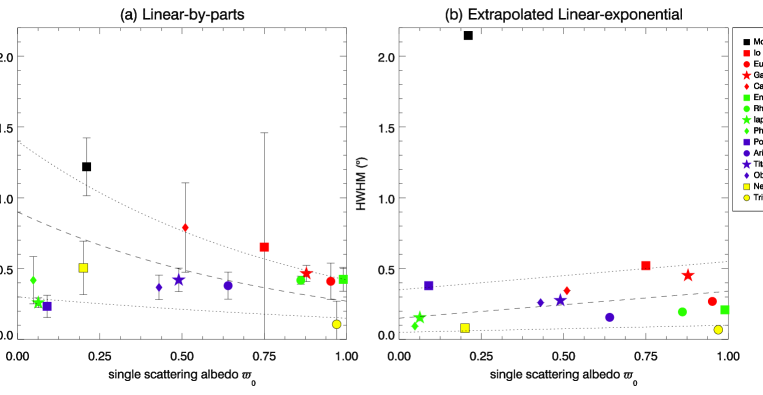
Figure 4: HWHM of the surge for satellites of Jupiter, Saturn, Uranus and Neptune derived with : (a) the linear-by-parts model and (b) the linear-exponential model convolved with the size of the Sun.
In (a) dashed line corresponds to a power-law fit to the data which is HWHM$\thicksim 0.9\times 0.3^{\varpi_{0}}$.
In (b) dashed line corresponds to a linear fit HWHM$\thicksim 0.15+0.19\varpi_{0}$.
Dotted lines are empirical functions to the boundaries of the data.

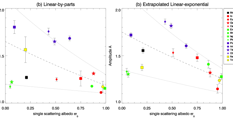
Figure 5: Amplitude of the surge derived with the linear-by-parts model for satellites of Jupiter, Saturn, Uranus and Neptune : (a) the linear-by-parts model and (b) the linear-exponential model convolved with the size of the Sun.
In (a) dashed line corresponds to a power fit to the data A$\thicksim 1.65\times 0.72^{\varpi_{0}}$
In (b) dashed line corresponds to the fit A$\thicksim 1.75\times 0.72^{\varpi_{0}}$.
Dotted lines are empirical functions to the data boundaries.

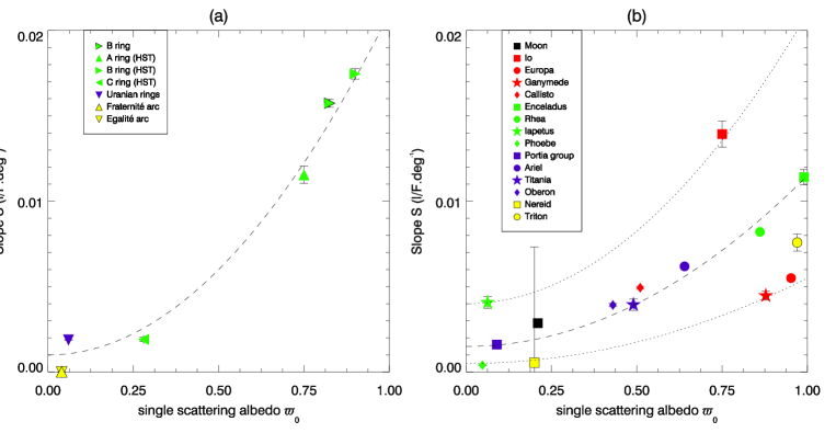
Figure 6: Morphological parameter S derived with the linear-by-parts model for : rings (a) and satellites (b) of Jupiter, Saturn, Uranus and Neptune.
In (a) dashed line corresponds to a power-law fit to the data which is S$\thicksim 0.001+0.02\varpi_{0}^{2}$
In (b) dashed line corresponds to a fit to the data which is S$\thicksim 0.001+0.01\varpi_{0}^{2}$.
Dotted lines are empirical functions to the data boundaries.

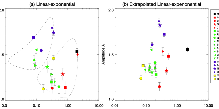
Figure 7: Cross comparison between the morphological parameters of the surge derived (a) with the linear-exponential model and (b) with the linear-exponential model convolved with the size of the Sun (see tables  7 and 6 of Appendix).
Dashed and dotted ellipses are arbitrary delimitations of the data points (see text).

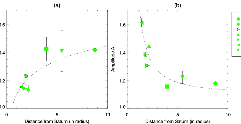
Figure 9: Variation of the morphological parameters: the amplitude A of the surge (a) and the half-width at half-maximum HWHM (b) derived with the linear-by-parts model with the distance from Saturn.
(Distances are taken from Murray and Dermott, 2000).

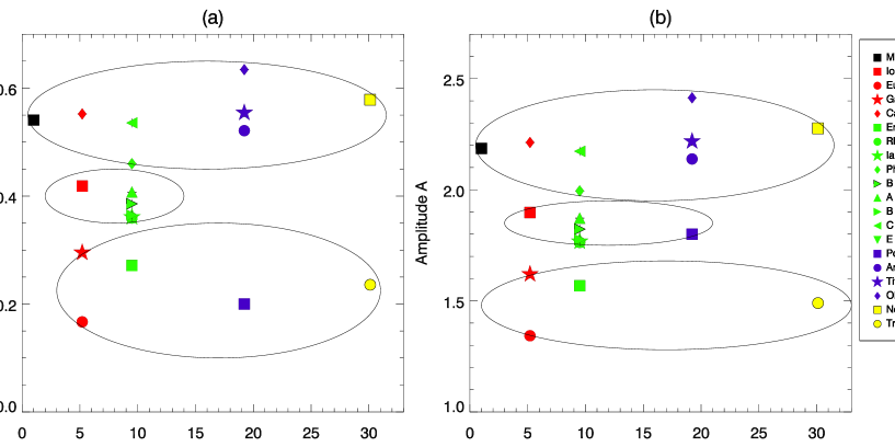
Figure 10: Variation of the morphological parameters: the amplitude A of the surge (a) and the half-width at half-maximum HWHM (b) derived with the logarithmic model fitted by the linear-by-parts model with the distance from Saturn.
(Distances are taken from Murray and Dermott, 2000).
Solid ellipses in (a) and (b) are arbitrary delimitations of the data points (see text).

Table 1: References for opposition phase curves of the selection of Solar System rings and satellites.

	Object	$\lambda$	References
		(nm)
	Moon	$\thicksim$570	(Whitaker, 1969; Rougier, 1933)
Jupiter	Main ring	$\thicksim$460	(Throop et al., 2004)
	Io	$\thicksim$570	(McEwen et al., 1988)
	Europa	$\thicksim$500	(Thompson and Lockwood, 1992)
	Ganymede	$\thicksim$600	(Morrison et al., 1974; Millis and Thompson, 1975; Blanco and Catalano, 1974)
	Callisto	$\thicksim$500	(Thompson and Lockwood, 1992)
Saturn	C ring	672	(French et al., 2007)
	B ring	$\thicksim$650	(Franklin and Cook, 1965)
	B ring (HST)	672	(French et al., 2007)
	A ring	672	(French et al., 2007)
	E ring	$\thicksim$650	(Pang et al., 1983; Larson, 1984; Showalter et al., 1991)
	Enceladus	439	(Verbiscer et al., 2005)
	Rhea	$\thicksim$500	(Domingue et al., 1995; Verbiscer and Veverka, 1989)
	Iapetus	$\thicksim$600	(Franklin and Cook, 1974)
	Phoebe	$\thicksim$650	(Bauer et al., 2006)
Uranus	Rings	$\thicksim$500	(Karkoschka, 2001)
	Portia group	$\thicksim$500	(Karkoschka, 2001)
	Ariel	$\thicksim$600	(Buratti et al., 1992; Karkoschka, 2001)
	Titania	$\thicksim$600	(Buratti et al., 1992; Karkoschka, 2001)
	Oberon	$\thicksim$600	(Buratti et al., 1992; Karkoschka, 2001)
Neptune	Fraternité	$\thicksim$500	(de Pater et al., 2005; Ferrari and Brahic, 1994)
	Egalité	$\thicksim$500	(de Pater et al., 2005; Ferrari and Brahic, 1994)
	Nereid	$\thicksim$570	(Schaefer and Tourtellotte, 2001)
	Triton	$\thicksim$400	(Buratti et al., 1991)

Table 2: Morphological parameters of opposition phase curves of Solar System objects. The unit of HWHM is the degree and the unit of the slope $S$ is I/F.deg^-1

	Object	Linear-by-parts fit			Linear-exponential fit
		A	HWHM	$S$	A	HWHM	$S$
	Moon	1.27	1.21	0.0261	1.53	1.98	0.0017
Jupiter	Main ring	1.23	2.68	0.0170	1.34	2.03	4.82$\times 10^{-8}$
	Io	1.25	0.65	0.0204	1.14	0.83	0.01500
	Europa	1.11	0.41	0.0095	1.13	0.31	0.0054
	Ganymede	1.31	0.46	0.0125	1.28	0.69	0.0040
	Callisto	1.25	0.78	0.0291	1.50	2.07	0.0024
Saturn	C ring	1.61	0.15	0.0342	1.55	0.09	0.0030
	B ring	1.30	0.23	0.0312	1.28	0.30	0.0155
	B ring (HST)	1.38	0.14	0.0278	1.37	0.09	0.0238
	A ring	1.44	0.13	0.0297	1.44	0.08	0.0159
	E ring	1.22	0.40	0.0903	1.51	0.86	1.19$\times 10^{-7}$
	Enceladus	1.15	0.42	0.0127	1.20	0.29	0.0113
	Rhea	1.17	0.41	0.0142	1.14	0.52	0.0080
	Iapetus	1.22	0.25	0.0348	1.36	0.22	0.0030
	Phoebe	1.17	0.41	0.0485	1.20	0.38	0.0003
Uranus	Rings	1.07	0.21	0.0274	1.08	0.45	0.0012
	Portia group	1.80	0.20	0.0015	1.48	0.13	0.0015
	Ariel	1.63	0.38	0.0178	1.60	0.18	0.0074
	Titania	1.67	0.45	0.0126	1.82	0.27	0.0032
	Oberon	1.77	0.37	0.0174	1.81	0.31	0.0037
Neptune	Fraternité	2.16	2.57	0.0136	1.86	1.50	1.10$\times 10^{-5}$
	Egalité	1.72	1.01	0.0160	1.77	0.67	8.34$\times 10^{-6}$
	Nereid	1.56	0.50	0.0042	1.45	0.34	0.0099
	Triton	1.17	0.10	0.0124	1.25	0.27	0.0049

Table 3: Direct output parameters of morphological models using opposition phase curves and ``ideal'' opposition phase curves of Solar System objects. The unit of $w$ is the degree and the unit of the slope $I_{s}$ is I/F.deg^-1

	Object	Logarithmic fit		Linear-exponential fit				Extrapolated linear-exponential fit
		$a_{0}$	$a_{1}$	$I_{p}$	$I_{b}$	$w$	$I_{s}$	$I_{p}$	$I_{b}$	$w$	$I_{s}$
	Moon	0.114	-0.015	0.048	0.090	1.433	0.0017	0.049	0.088	1.548	0.0016
Jupiter	Main ring	3.9$\times 10^{-6}$	-5.6$\times 10^{-7}$	1.1$\times 10^{-6}$	3.2$\times 10^{-6}$	1.470	4.8$\times 10^{-8}$	2.4$\times 10^{-6}$	3.2$\times 10^{-6}$	0.905	4.6$\times 10^{-8}$
	Io	0.726	-0.077	0.100	0.699	0.600	0.0150	0.313	0.652	0.375	0.0107
	Europa	0.580	-0.025	0.076	0.572	0.230	0.0054	0.086	0.573	0.193	0.0055
	Ganymede	0.379	-0.028	0.100	0.349	0.500	0.0040	0.114	0.355	0.325	0.0041
	Callisto	0.182	-0.025	0.070	0.140	1.500	0.0024	0.091	0.171	0.248	0.0051
Saturn	C ring	0.056	-0.007	0.033	0.059	0.070	0.0030	0.031	0.056	0.104	0.0021
	B ring	0.506	-0.050	0.142	0.502	0.223	0.0155	0.179	0.511	0.143	0.0174
	B ring (HST)	0.628	-0.058	0.249	0.656	0.066	0.0238	0.213	0.647	0.094	0.0216
	A ring	0.390	-0.046	0.182	0.409	0.060	0.0159	0.150	0.401	0.093	0.0143
	E ring	2.1$\times 10^{-6}$	-5.2$\times 10^{-7}$	9.3$\times 10^{-7}$	1.8$\times 10^{-6}$	0.623	1.2$\times 10^{-7}$	4.8$\times 10^{-7}$	1.2$\times 10^{-6}$	1.085	3.8$\times 10^{-7}$
	Enceladus	0.912	-0.063	0.180	0.895	0.215	0.0113	0.251	0.899	0.150	0.0116
	Rhea	0.602	-0.055	0.085	0.573	0.379	0.0080	0.236	0.576	0.139	0.0082
	Iapetus	0.112	-0.010	0.039	0.110	0.160	0.0030	0.035	0.116	0.111	0.0039
	Phoebe	0.007	-0.0001	0.001	0.008	0.276	0.0003	0.002	0.008	0.067	0.0004
Uranus	Rings	0.038	-0.004	0.003	0.044	0.326	0.0012	0.014	0.045	0.017	0.0012
	Portia group	0.058	-0.006	0.026	0.055	0.100	0.0015	0.038	0.054	0.273	0.0010
	Ariel	0.366	-0.044	0.213	0.355	0.129	0.0074	0.217	0.359	0.112	0.0077
	Titania	0.252	-0.034	0.181	0.221	0.198	0.0032	0.181	0.221	0.198	0.0032
	Oberon	0.236	-0.034	0.168	0.208	0.229	0.0037	0.181	0.211	0.186	0.0040
Neptune	Fraternité	0.0005	-0.0001	0.00037	0.00043	1.082	1.1$\times 10^{-5}$	0.00086	0.00022	1.1$\times 10^{-5}$	5.6$\times 10^{-6}$
	Egalité	0.0001	-0.001	0.00040	0.00052	0.489	8.3$\times 10^{-6}$	0.00090	0.00021	1.106	1.5$\times 10^{-5}$
	Nereid	0.144	-0.021	0.064	0.140	0.250	0.0099	0.065	0.175	0.057	0.0301
	Triton	0.584	-0.035	0.140	0.560	0.200	0.0049	0.146	0.609	0.049	0.0075

Table 4: References for the single scattering albedo of Solar System objects.

	Object	$\varpi_{0}$	$\lambda$	References
			(nm)
	Moon	0,21	$\thicksim$500	(Helfenstein et al., 1997)
Jupiter	Io	0,75	590	(McEwen et al., 1988)
	Europa	0,96	550	(Domingue and Verbiscer, 1997)
	Ganymede	0,87	470	(Domingue and Verbiscer, 1997)
	Callisto	0,53	470	(Domingue and Verbiscer, 1997)
Saturn	C ring	0,16	672	(French et al., 2007)
	B ring	0,83	672	(Poulet et al., 2002)
	B ring (HST)	0,85	672	(French et al., 2007)
	A ring	0,79	672	(French et al., 2007)
	Enceladus	0,99	480	(Verbiscer and Veverka, 1991)
	Rhea	0,86	480	(Verbiscer and Veverka, 1989)
	Iapetus	0,16	480	(Buratti, 1984)
	Phoebe	0,06	480	(Simonelli et al., 1999)
Uranus	Rings	0,06	$\thicksim$500	(Karkoschka, 2001)
	Portia group	0,09	$\thicksim$500	(Karkoschka, 2001)
	Ariel	0,64	$\thicksim$500	(Karkoschka, 2001)
	Titania	0,48	$\thicksim$475	(Veverka et al., 1987)
	Oberon	0,43	$\thicksim$500	(Karkoschka, 2001)
Neptune	Fraternité	0,02	480	(Ferrari and Brahic, 1994)
	Egalité	0,02	480	(Ferrari and Brahic, 1994)
	Nereid	0,21	$\thicksim$500	(Thomas et al., 1991)
	Triton	0,97	500	(Lee et al., 1992)

Table 5: Morphological parameters of ``ideal'' opposition phase curves of Solar System objects. The unit of HWHM is the degree and the unit of the slope $S$ is I/F.deg^-1

	Object	Linear-by-parts and log fits			Extrapolated linear-exponential fit
		A	HWHM	$S$	A	HWHM	$S$
	Moon	2.18	0.54	0.0224	1.55	2.14	0.0016
Jupiter	Main ring	2.21	0.55	0.0230	1.76	1.25	4.55$\times 10^{-8}$
	Io	1.89	0.41	0.0169	1.47	0.52	0.0107
	Europa	1.34	0.16	0.0064	1.15	0.26	0.0055
	Ganymede	1.62	0.29	0.0117	1.32	0.45	0.0041
	Callisto	2.21	0.55	0.0229	1.53	0.34	0.0051
Saturn	C ring	2.17	0.53	0.0221	1.54	0.14	0.0021
	B ring	1.82	0.38	0.0155	1.35	0.19	0.0174
	B ring (HST)	1.77	0.36	0.0146	1.32	0.13	0.0216
	A ring	1.87	0.40	0.0165	1.37	0.12	0.0143
	E ring	3.38	0.99	0.0450	2.80	1.50	3.76$\times 10^{-7}$
	Enceladus	1.56	0.27	0.0107	1.27	0.20	0.0116
	Rhea	1.76	0.35	0.0144	1.41	0.19	0.0082
	Iapetus	1.76	0.36	0.0145	1.30	0.15	0.0039
	Phoebe	1.99	0.45	0.0187	1.33	0.09	0.0004
Uranus	Rings	1.98	0.45	0.0186	1.31	0.02	0.0012
	Portia group	1.80	0.20	0.0015	1.71	0.37	0.0010
	Ariel	2.13	0.52	0.0215	1.60	0.15	0.0077
	Titania	2.21	0.55	0.0230	1.81	0.27	0.0032
	Oberon	2.41	0.63	0.0267	1.86	0.25	0.0040
Neptune	Fraternité	2.72	0.75	0.0314	4.99	1.53	5.61$\times 10^{-6}$
	Egalité	2.39	0.62	0.0253	5.34	1.53	1.53$\times 10^{-5}$
	Nereid	2.27	0.57	0.0241	1.37	0.08	0.0301
	Triton	1.49	0.23	0.0092	1.23	0.06	0.0075

APPENDIX :
REFINEMENTS TO THE SUN'S ANGULAR SIZE EFFECT To compute the distance from a Solar System object to the Sun at any given date, it is not appropriate to use the semi-major axis. We use a series of equations which take into consideration the distance between the Sun and the planet at the approximate date. The heliocentric radius $r_{\textrm{p}}$, the distance from the focus of the ellipse (i.e. the Sun) to the planet, is given by:

$$r_{\textrm{p}}=a(1-e\cos E)$$ (10)

where $E$ is the eccentric anomaly, $a$ and $e$ are two of the seven orbital elements which define an ellipse in space : $a$ is the mean distance, or the value of the semi-major axis of the orbit (average Sun to planet distance); $e$ is the eccentricity of the ellipse which describes the orbit (dimensionless); $i$ is the inclination (in degrees), or angle between the plane of the ecliptic (the plane of the Earth's orbit about the Sun) and the plane of the planets orbit; $\Omega$ is the longitude of ascending node (in degrees), or the position in the orbit where the elliptical path of the planet passes through the plane of the ecliptic, from below the plane to above the plane; $\tilde{\omega}$ is the longitude of perihelion (in degrees), or the position in the orbit where the planet is closest to the Sun; $\lambda$ is the mean longitude (in degrees), the position of the planet in the orbit; and $M$ is mean anomaly (in degrees). The mean anomaly gives the planet's angular position for a circular orbit with radius equal to the semi major axis. It is computed directly from the elements using:

$$M=\lambda-\tilde{\omega}$$ (11)

Kepler's second law states that the radius vector of a planet sweeps out equal areas in equal times. The planet must speed up and slow down in its orbit. The true anomaly $f$ gives the planet's actual angular position in its orbit. It is the angle (at the Sun) between perihelion of the orbit and the current location of the planet. To obtain its value, first we compute the eccentric anomaly, $E$, from $M$ and the eccentricity $e$ by using the ``Kepler equation'':

$$M=E-e\sin E$$ (12)

An expansion to order $e^{3}$ of the solution to the ``Kepler equation'' is:

$$E=M+(e-\frac{e^{3}}{8})\sin M+\frac{1}{2}e^{2}\sin 2M+\frac{3}{8}e^{3}\sin 3M$$ (13)

Now, to find the orbital elements of a planet at a specific date, we use:

$$a = a_{0}+\dot{a}t$$ (14)

$$e = e_{0}+\dot{e}t$$ (15)

$$i = i_{0}+\left(\dot{a}/3600\right)t$$ (16)

$$\tilde{\omega} = \tilde{\omega}_{0}+\left(\dot{\tilde{\omega}}/3600\right)t$$ (17)

$$\Omega = \Omega_{0}+\left(\dot{\Omega}/3600\right)t$$ (18)

$$\lambda = \lambda_{0}+\left(\dot{\lambda}/3600+360~{}N_{r}\right)t$$ (19)

where $t$ is the observation time (Table Appendix6) converted in Julian centuries since JD 2451545.0, the zero index quantities are the orbital elements at the epoch of J2000 (JD 2451545.0) and the dot quantities are the change per julian century of the orbital elements (values are taken in Murray and Dermott, 2000). When we have the heliocentric radius at the given observation time, we can compute the solar angular size $\alpha_{\odot}$ using $r_{p}$ and $r_{\odot}$, the radius of the Sun:

$$\alpha_{\odot}=\arcsin\frac{r_{\odot}}{r_{p}}$$ (20)

The limb darkening function of Pierce and Waddell (1961) has been used in the past to be convolved with a theoretical opposition effect function (Kawata and Irvine, 1974). Its formula is:

$$W(\mu^{\prime})=a_{\lambda}+b_{\lambda}\mu^{\prime}+c_{\lambda}\left[1-\mu^{\prime}\cdot\log\left(1+\frac{1}{\mu^{\prime}}\right)\right]$$ (21)

where $\mu^{\prime}=\cos\theta^{\prime}$ and $\theta^{\prime}$ varies from 0 to the Sun's angular radius $\alpha_{\odot}$. $a_{\lambda}$, $b_{\lambda}$ and $c_{\lambda}$ are coefficients that depend on the wavelength (values are given in table Appendix7). We perform a normalized convolution of the limb darkening function to the linear-exponential function $P(\alpha)$ by doing:

$$P^{\prime}(\alpha)=\frac{\int_{0}^{\alpha_{\odot}}P(\alpha)\cdot W(\cos\theta^{\prime})d\theta^{\prime}}{\int_{0}^{\alpha_{\odot}}W(\cos\theta^{\prime})d\theta^{\prime}}$$ (22)

Table 6: References for the observational parameters needed to compute the angular size of the Sun $\alpha_{\odot}$. Bold text corresponds to missing data replaced arbitrarily, we assumed an hourly time of 18:00:00.0

	Object	Solar Angular Size	Observation Time	References
		$\alpha_{\odot}$(o)	UT
	Moon	0.263	1968 December 24	(Whitaker, 1969)
Jupiter	Main ring	0.0506	2000 December 13	(Throop et al., 2004)
	Io	0.0498	1977 December 15	(Lockwood et al., 1980)
	Europa	0.0515	1976 January 1	(Thompson and Lockwood, 1992)
	Ganymede	0.0499	1971 may 1	(Blanco and Catalano, 1974)
	Callisto	0.0515	1976 January 1	(Thompson and Lockwood, 1992)
Saturn	C ring	0.0295	2005 January 13	(French et al., 2007)
	B ring	0.0266	1959 June 26	(Franklin and Cook, 1965)
	B ring (HST)	0.0295	2005 January 13	(French et al., 2007)
	A ring	0.0295	2005 January 13	(French et al., 2007)
	E ring	0.0271	1980 January 1	(Larson, 1984)
	Enceladus	0.0287	1997 October 10	(Verbiscer et al., 2005)
	Rhea	0.0268	1976 January 13	(Lockwood et al., 1980)
	Iapetus	0.0266	1972 December 1	(Franklin and Cook, 1974)
	Phoebe	0.0295	2005 January 13	(Bauer et al., 2006)
Uranus	Rings	0.0138	1997 July 29	(Karkoschka, 2001)
	Portia group	0.0138	1997 July 29	(Karkoschka, 2001)
	Ariel	0.0138	1997 July 29	(Karkoschka, 2001)
	Titania	0.0138	1997 July 29	(Karkoschka, 2001)
	Oberon	0.0138	1997 July 29	(Karkoschka, 2001)
Neptune	Fraternité	0.00885	2002 July 27	(de Pater et al., 2005)
	Egalité	0.00885	2002 July 27	(de Pater et al., 2005)
	Nereid	0.00889	1998 June 20	(Schaefer and Tourtellotte, 2001)
	Triton	0.00885	1988 June 20	(Buratti et al., 1991)

Table 7: Parameters of the limb darkening function of Pierce and Waddell (1961) at similar wavelengths to the observations.

	Object		Pierce and Waddell (1961)
		$\lambda_{\textrm{obs}}$	$\lambda$	$a_{\lambda}$	$b_{\lambda}$	$c_{\lambda}$
		(nm)	(nm)
	Moon	$\thicksim$570	560	0.75079	0.41593	-0.54334
Jupiter	Main ring	$\thicksim$460	460	0.58274	0.56078	-0.46772
	Io	$\thicksim$570	560	0.75079	0.41593	-0.54334
	Europa	$\thicksim$500	500	0.68897	0.47873	-0.54651
	Ganymede	$\thicksim$600	600	0.78074	0.38427	-0.53777
	Callisto	$\thicksim$500	500	0.68897	0.47873	-0.54651
Saturn	C ring	672	660	0.83717	0.33283	-0.55400
	B ring	$\thicksim$650	640	0.81999	0.34918	-0.55132
	B ring (HST)	672	660	0.83717	0.33283	-0.55400
	A ring	672	660	0.83717	0.33283	-0.55400
	E ring	$\thicksim$650	640	0.81999	0.34918	-0.55132
	Enceladus	439	440	0.49375	0.62584	-0.38974
	Rhea	$\thicksim$500	500	0.68897	0.47873	-0.54651
	Iapetus	$\thicksim$600	600	0.78074	0.38427	-0.53777
	Phoebe	$\thicksim$650	640	0.81999	0.34918	-0.55132
Uranus	Rings	$\thicksim$500	500	0.68897	0.47873	-0.54651
	Portia group	$\thicksim$500	500	0.68897	0.47873	-0.54651
	Ariel	$\thicksim$600	600	0.78074	0.38427	-0.53777
	Titania	$\thicksim$600	600	0.78074	0.38427	-0.53777
	Oberon	$\thicksim$600	600	0.78074	0.38427	-0.53777
Neptune	Fraternité	$\thicksim$500	500	0.68897	0.47873	-0.54651
	Egalité	$\thicksim$500	500	0.68897	0.47873	-0.54651
	Nereid	$\thicksim$570	560	0.75079	0.41593	-0.54334
	Triton	$\thicksim$400	400	0.16732	0.84347	-0.03516

References

- Bauer et al. (2006) Bauer, J. M., Grav, T., Buratti, B. J., Hicks, M. D., Sep. 2006. The phase curve survey of the irregular saturnian satellites: A possible method of physical classification. Icarus 184, 181–197.
- Belskaya et al. (2008) Belskaya, I. N., Levasseur-Regourd, A.-C., Shkuratov, Y. G., Muinonen, K., 2008. Surface Properties of Kuiper Belt Objects and Centaurs from Photometry and Polarimetry. The Solar System Beyond Neptune, pp. 115–127.
- Belskaya and Shevchenko (2000) Belskaya, I. N., Shevchenko, V. G., Sep. 2000. Opposition Effect of Asteroids. Icarus 147, 94–105.
- Blanco and Catalano (1974) Blanco, C., Catalano, S., Jun. 1974. On the photometric variations of the Saturn and Jupiter satellites. Astronomy & Astrophysics 33, 105–111.
- Bobrov (1970) Bobrov, M. S., 1970. Physical properties of Saturn's rings. In: Surfaces and interiors of planets and satellites, edited by A. Dollfus (Academic, New York). pp. 376–461.
- Buratti (1984) Buratti, B. J., Sep. 1984. Voyager disk resolved photometry of the Saturnian satellites. Icarus 59, 392–405.
- Buratti and Veverka (1985) Buratti, B. J., 1985. Photometry of rough planetary surfaces : The role of multiple scattering. Icarus 64, 320–328.
- Buratti et al. (1992) Buratti, B. J., Gibson, J., Mosher, J. A., Oct. 1992. CCD photometry of the Uranian satellites. Astronomical Journal 104, 1618–1622.
- Buratti et al. (1991) Buratti, B. J., Lane, A. L., Gibson, J., Burrows, H., Nelson, R. M., Bliss, D., Smythe, W., Garkanian, V., Wallis, B., Oct. 1991. Triton's surface properties - A preliminary analysis from ground-based, Voyager photopolarimeter subsystem, and laboratory measurements. Journal of Geophysical Research Supplement 96, 19197–+.
- Buratti et al. (1988) Buratti, B. J., Nelson, R. M., Lane, A. L., May 1988. Surficial textures of the Galilean satellites. Nature 333, 148–151.
- Burns et al. (1999) Burns, J. A., Showalter, M. R., Hamilton, D. P., Nicholson, P. D., de Pater, I., Ockert-Bell, M. E., Thomas, P. C., May 1999. The Formation of Jupiter's Faint Rings. Science 284, 1146–+.
- Chandrasekhar (1960) Chandrasekhar, S. 1960. Radiative transfer. New York (Dover).
- Colwell and Esposito (1992) Colwell, J. E., Esposito, L. W., Jun. 1992. Origins of the rings of Uranus and Neptune. I - Statistics of satellite disruptions. Journal of Geophysical Research 97, 10227–+.
- Colwell and Esposito (1993) Colwell, J. E., Esposito, L. W., Apr. 1993. Origins of the rings of Uranus and Neptune. II - Initial conditions and ring moon populations. Journal of Geophysical Research 98, 7387–7401.
- Cooke (1991) Cooke, M. L., 1991. Saturn's rings: Photometric studies of the C Ring and radial variation in the Keeler Gap. Ph.D. thesis, AA(Cornell Univ., Ithaca, NY.).
- Croft et al. (1995) Croft, S. K., Kargel, J. S., Kirk, R. L., Moore, J. M., Schenk, P. M., Strom, R. G., 1995. The geology of Triton. In: Neptune and Triton. pp. 879–947.
- Cuzzi and Estrada (1998) Cuzzi, J. N., Estrada, P. R., Mar. 1998. Compositional Evolution of Saturn's Rings Due to Meteoroid Bombardment. Icarus 132, 1–35.
- Déau et al. (2008) D au, E., Charnoz, S., Dones, L., Brahic, A., Porco, C. C., 2008. ISS/Cassini observes the opposition effect in Saturn's rings: I. Morphology of optical phase curves. Icarus submited in April 2007 and corrected in May 2008.
- de Pater et al. (2005) de Pater, I., Gibbard, S. G., Chiang, E., Hammel, H. B., Macintosh, B., Marchis, F., Martin, S. C., Roe, H. G., Showalter, M., Mar. 2005. The dynamic neptunian ring arcs: evidence for a gradual disappearance of Liberté and resonant jump of courage. Icarus 174, 263–272.
- Domingue and Verbiscer (1997) Domingue, D., Verbiscer, A., Jul. 1997. Re-Analysis of the Solar Phase Curves of the Icy Galilean Satellites. Icarus 128, 49–74.
- Domingue et al. (1995) Domingue, D. L., Lockwood, G. W., Thompson, D. T., Jun. 1995. Surface textural properties of icy satellites: A comparison between Europa and Rhea. Icarus 115, 228–249.
- Dones et al. (1993) Dones, L., Cuzzi, J. N., Showalter, M. R., Sep. 1993. Voyager Photometry of Saturn's A Ring. Icarus 105, 184–215.
- Doyle et al. (1989) Doyle, L. R., Dones, L., Cuzzi, J. N., Jul. 1989. Radiative transfer modeling of Saturn's outer B ring. Icarus 80, 104–135.
- Esposito et al. (1979) Esposito, L. W., Lumme, K., Benton, W. D., Martin, L. J., Ferguson, H. M., Thompson, D. T., Jones, S. E., Sep. 1979. International planetary patrol observations of Saturn's rings. II - Four color phase curves and their analysis. Astronomical Journal 84, 1408–1415.
- Ferrari and Brahic (1994) Ferrari, C., Brahic, A., Sep. 1994. Azimuthal brightness asymmetries in planetary rings. 1: Neptune's arcs and narrow rings. Icarus 111, 193–210.
- Franklin and Cook (1974) Franklin, F. A., Cook, A. F., Nov. 1974. Photometry of Saturn's satellites - The opposition effect of Iapetus at maximum light and the variability of Titan. Icarus 23, 355–362.
- Franklin and Cook (1965) Franklin, F. A., Cook, F. A., Nov. 1965. Optical properties of Saturn's rings. II. Two-color phase curves of the 2 bright rings. Astronomical Journal 70, 704–+.
- French and Nicholson (1995) French, R. G., Nicholson, P. D., May 1995. Edge waves and librations in the Uranus epsilon ring. In: Bulletin of the American Astronomical Society. Vol. 27 of Bulletin of the American Astronomical Society. pp. 857–+.
- French et al. (2007) French, R. G., Verbiscer, A., Salo, H., McGhee, C., Dones, L., Jun. 2007. Saturn's Rings at True Opposition. The Publications of the Astronomical Society of the Pacific 119, 623–642.
- Hapke (1984) Hapke, B., Jul. 1984. Bidirectional reflectance spectroscopy. III - Correction for macroscopic roughness. Icarus 59, 41–59.
- Hapke (1986) Hapke, B., Aug. 1986. Bidirectional reflectance spectroscopy. IV - The extinction coefficient and the opposition effect. Icarus 67, 264–280.
- Hapke (2002) Hapke, B., Jun. 2002. Bidirectional Reflectance Spectroscopy5. The Coherent Backscatter Opposition Effect and Anisotropic Scattering. Icarus 157, 523–534.
- Hapke et al. (1996) Hapke, B., Dimucci, D., Nelson, R., Smythe, W., Mar. 1996. The Nature of the Opposition Effect in Frost, Vegetation and Soils. In: Lunar and Planetary Institute Conference Abstracts. Vol. 27 of Lunar and Planetary Inst. Technical Report. pp. 491–+.
- Harris et al. (1989a) Harris, A. W., Young, J. W., Bowell, E., Martin, L. J., Millis, R. L., Poutanen, M., Scaltriti, F., Zappala, V., Schober, H. J., Debehogne, H., Zeigler, K. W., Jan. 1989a. Photoelectric observations of asteroids 3, 24, 60, 261, and 863. Icarus 77, 171–186.
- Harris et al. (1989b) Harris, A. W., Young, J. W., Contreiras, L., Dockweiler, T., Belkora, L., Salo, H., Harris, W. D., Bowell, E., Poutanen, M., Binzel, R. P., Tholen, D. J., Wang, S., Oct. 1989b. Phase relations of high albedo asteroids - The unusual opposition brightening of 44 NYSA and 64 Angelina. Icarus 81, 365–374.
- Helfenstein et al. (1997) Helfenstein, P., Veverka, J., Hillier, J., Jul. 1997. The Lunar Opposition Effect: A Test of Alternative Models. Icarus 128, 2–14.
- Ip (1983) Ip, W.-H., May 1983. Collisional interactions of ring particles - The ballistic transport process. Icarus 54, 253–262.
- Irvine (1966) Irvine, W. M., 1966. The shadowing effect in diffuse reflection. Journal of Geophysical Research 71, 2931–2937.
- Kaasalainen (2003) Kaasalainen, S., Oct. 2003. Laboratory photometry of planetary regolith analogs. I. Effects of grain and packing properties on opposition effect. Astronomy and Astrophysics 409, 765–769.
- Kaasalainen et al. (2001) Kaasalainen, S., Muinonen, K., Piironen, J., Aug. 2001. Comparative study on opposition effect of icy solar system objects. Journal of Quantitative Spectroscopy and Radiative Transfer 70, 529–543.
- Karkoschka (2001) Karkoschka, E., May 2001. Comprehensive Photometry of the Rings and 16 Satellites of Uranus with the Hubble Space Telescope. Icarus 151, 51–68.
- Kawata and Irvine (1974) Kawata, Y., Irvine, W. M., 1974. Models of Saturn's rings which satisfy the optical observations. In: Woszczyk, A., Iwaniszewska, C. (Eds.), Exploration of the Planetary System. Vol. 65 of IAU Symposium. pp. 441–464.
- Larson (1984) Larson, S., 1984. Summary of Optical Ground-Based E Ring Observations at the University of Arizona. In: Greenberg, R., Brahic, A. (Eds.), IAU Colloq. 75: Planetary Rings. pp. 111–+.
- Lee et al. (1992) Lee, P., Helfenstein, P., Veverka, J., McCarthy, D., Sep. 1992. Anomalous-scattering region on Triton. Icarus 99, 82–97.
- Lissauer et al. (1988) Lissauer, J. J., Squyres, S. W., Hartmann, W. K., Nov. 1988. Bombardment history of the Saturn system. Journal of Geophysical Research 93, 13776–13804.
- Lockwood et al. (1980) Lockwood, G. W., Thompson, D. T., Lumme, K., Jul. 1980. A possible detection of solar variability from photometry of Io, Europa, Callisto, and Rhea, 1976-1979. Astronomical Journal 85, 961–968.
- Lumme and Irvine (1976) Lumme, K., Irvine, W. M., Oct. 1976. Photometry of Saturn's rings. Astronomical Journal 81, 865–893.
- Lumme et al. (1990) Lumme, K., Peltoniemi, J., Irvine, W. M., 1990. Some photometric techniques for atmosphereless solar system bodies. Advances in Space Research 10, 187–193.
- McCord et al. (2001) McCord, T. B., Hansen, G. B., Hibbitts, C. A., May 2001. Hydrated Salt Minerals on Ganymede's Surface: Evidence of an Ocean Below. Science 292, 1523–1525.
- McEwen et al. (1988) McEwen, A. S., Soderblom, L. A., Johnson, T. V., Matson, D. L., Sep. 1988. The global distribution, abundance, and stability of SO2 on Io. Icarus 75, 450–478.
- Millis and Thompson (1975) Millis, R. L., Thompson, D. T., Dec. 1975. UBV photometry of the Galilean satellites. Icarus 26, 408–419.
- Mishchenko (1992) Mishchenko, M. I., Aug. 1992. The angular width of the coherent back-scatter opposition effect - an application to icy outer planet satellites. Astrophysics and Space Science 194, 327–333.
- Mishchenko (1993) Mishchenko, M. I., Jul. 1993. On the nature of the polarization opposition effect exhibited by Saturn's rings. Astrophysical Journal 411, 351–361.