Dynamical Fine Tuning in Brane Inflation

Abstract

We investigate a novel mechanism of dynamical tuning of a flat potential in the open string landscape within the context of warped brane-antibrane inflation in type IIB string theory. Because of competing effects between interactions with the moduli stabilizing $D7$-branes in the warped throat and anti-$D3$-branes at the tip, a stack of branes gives rise to a local minimum of the potential, holding the branes high up in the throat. As branes successively tunnel out of the local minimum to the bottom of the throat the potential barrier becomes lower and is eventually replaced by a flat inflection point, around which the remaining branes easily inflate. This dynamical flattening of the inflaton potential reduces the need to fine tune the potential by hand, and also leads to successful inflation for a larger range of inflaton initial conditions, due to trapping in the local minimum.

I Introduction

The suitability of a scalar field potential for inflation is sensitive to the form of nonrenormalizable interactions: even if their effects are Planck-suppressed, a correction to the inflaton mass of order $V/M_{p}^{2}$ is enough to spoil inflation. Therefore it makes sense to use ultraviolet (UV) complete theories such as string theory to compute the form of, and possible corrections to, inflationary potentials and models. Important progress has been made in the last few years in refining string theoretic models of inflation, especially those based on the motion of a mobile $D3$ brane in the extra, compact dimensions Dvali and Tye (1999); Kachru et al. (2003); Baumann et al. (2006); Burgess et al. (2007); Baumann et al. (2008); Krause and Pajer (2008); Panda et al. (2007); Ali et al. (2009); Baumann et al. (2009). Increasingly, assumptions about the form of the inflaton potential that were necessary to make initial progress are being replaced by calculations of the potential from effective field theory and AdS/CFT techniques arising from string theory constructions.

Despite this progress (or rather because of it), several fine-tuning challenges typical in usual inflationary model building which can be sensitive to UV-physics still remain, namely fine-tuning of the precise functional form of the potential and of the initial conditions of the inflaton field. In Figure 1 we illustrate the problem of functional fine-tuning for the brane inflationary scenario of Baumann et al. (2008): for one set of parameter values, the potential has an inflection point which is flat enough to support a sufficient number of e-folds of inflation (labeled (b)), while small deviations from these parameters ((a) and (c)) can lead to a potential which does not support inflation.

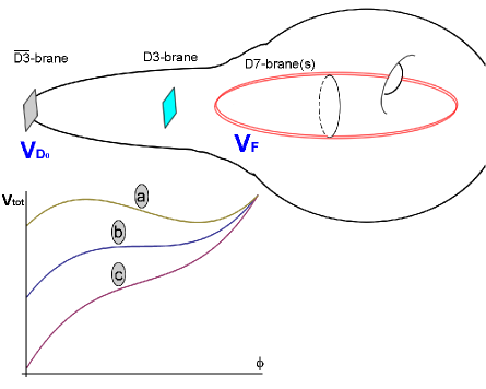
Figure 1: Warped brane inflation suffers from a fine tuning problem due to the fact that small changes in parameters (a)-(c) lead to drastic changes in the behavior of the potential which make it unsuitable for inflation.

In addition to the functional fine tuning of the potential, small field inflation models such as brane inflation in which the inflaton ranges over sub-Planckian field values typically also suffer from an overshoot problem. This occurs when the initial conditions are such that the inflaton has too much kinetic energy when it enters the inflationary region to satisfy the slow roll conditions, and it overshoots the slow roll region (for a recent discussion of the overshoot problem in string theory models of inflation, see Linde and Westphal (2008); Itzhaki and Kovetz (2007); Underwood (2008); Itzhaki (2008)). This problem is particularly acute for the inflection-point type of inflationary potentials which arise from the brane constructions of Baumann et al. (2008).

From the point of view of the 4-dimensional effective theory, the fine tuning in both the potential and initial conditions must be done by hand. However, since the potential originates from a higher dimensional string theoretic model, it is interesting to investigate whether this tuning can arise in a dynamical way. One method of dynamical tuning commonly used in string theoretic constructions is that of the landscape; as one moves, by tunneling or rolling, in the multidimensional field space the parameters of the theory (such as the fluxes wrapped on cycles in the internal space) change in a dynamic way.

In this paper we will consider a mechanism of dynamical resolution of these fine tuning problems in the open string landscape; we will focus on the specific model in which brane inflation arises as the interaction between $D3$- and $\overline{D}3$-branes in a locally warped throat in the presence of moduli stabilizing ingredients such as $D7$-branes Baumann et al. (2008), as shown schematically in Figure 1. Recently it was shown that the (relative) functional fine tuning problem in this model is greatly ameliorated for certain optimal values of the parameters Hoi and Cline (2009): near this optimal region, each parameter could vary at the level of a part in a few without spoiling inflation. Nevertheless, once the full allowed field range is included correctly the model still requires fine tuning of the initial conditions to avoid overshooting the inflationary region of the inflection point.

Revisiting a novel mechanism, first suggested in Cline and Stoica (2005), we will show that in the presence of sufficiently many branes and anti-branes the potential typically develops a local minimum that serves to trap the branes at a finite distance in the throat. The local minimum arises because of a competition between the backreaction of the $D3$-branes on the four cycle volume and the attractive force of the antibranes at the tip of the throat. Individual branes have a finite probability to tunnel out of the local minimum and annihilate with the antibranes at the tip, and as they do so they change the balance of forces on the remaining branes. As the number of trapped branes decreases so does the height of the potential barrier of the local minimum, until at some point the local minimum disappears and is replaced with an inflection point potential. This scenario is shown schematically in Figure 2.

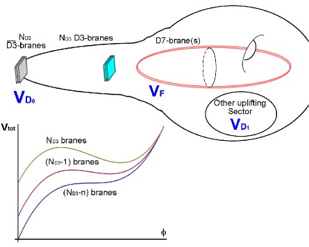
Figure 2: In the presence of multiple branes and antibranes, the inflationary potential develops a local minimum which traps the branes at a finite distance in the throat. As individual branes tunnel out of the local minimum the potential barrier decreases, until the potential forms a flat inflection point. This dynamical process can aid in reducing the amount of necessary fine-tuning of the parameters in the potential, and can also help to reduce the overshoot problem.

The tunneling of the branes and subsequent modification to the potential is equivalent to scanning over parameters of the potential in a dynamical way. As long as other sectors dominate the uplifting energy, the step size can be sufficiently small and we can dynamically access the parameters needed to obtain a sufficient amount of inflation, alleviating the parameter fine tuning problem. Moreover, prior to the inflationary period, as mobile $D$-branes fall into the throat they are naturally trapped in the local minimum, both due to requirement of large enough kinetic energy to overcome the potential barrier as well as due to energy loss in collisions with other trapped $D$-branes Kofman et al. (2004); McAllister and Mitra (2005). This leads to a relaxation of the overshoot problem. The original scenario Cline and Stoica (2005) was incomplete because important stringy corrections to the nonperturbative superpotential for the $D3$ brane position in the throat were not yet known. Our new observation is that the dynamical tuning mechanism does in fact exist when these corrections are taken into account.

The paper is organized as follows. In Section II we review the form of the inflationary potential, and illustrate the functional and initial conditions fine-tuning problems. In Section III we demonstrate the mechanism in which the potential is dynamically flattened, and discuss how this can help in relaxing the amount of functional and initial conditions fine-tuning for this model. We also discuss the constraints on the parameters of the model for the rate of the dynamical tunneling process to be faster than other decay rates, and find these constraints to be quite strong. Finally, in Section IV we summarize our findings.

II Potential for D-brane Inflation

The model of type IIB $D3$-brane inflation we will consider consists of several ingredients Dvali and Tye (1999); Kachru et al. (2003); Baumann et al. (2008); Krause and Pajer (2008); Burgess et al. (2007):

• Stacks of spacetime filling $D3$- and $\overline{D3}$-branes, where the radial separation between the branes serves as the inflaton field and the energy from the non-BPS $\overline{D3}$-branes provide the inflationary energy. In particular, for simplicity we will consider $N_{D3}$ mobile $D3$-branes and the same number of $\overline{D3}$-branes. If this is not the case then the energy from reheating is trapped on the remaining branes at the tip, so reheating of the standard model sector does not occur unless the standard model itself is realized in this throat, and it is not known whether this is possible. In contrast, if there are no branes remaining in the inflationary throat after inflation then the inflationary energy is channeled into closed string modes Barnaby et al. (2005); Chialva et al. (2006); Kofman and Yi (2005); Chen and Tye (2006); Berndsen et al. (2008) that may reheat the standard model, which can be constructed elsewhere in the compact space. Our results, however, will not be sensitive to this assumption because it only changes the dependence on the number of $D3$-branes in the subdominant Coulomb attraction, and it is straightforward to generalize the scenario.

• A warped throat, which suppresses the attractive Coulombic force between the $D3-\overline{D3}$ pair and provides a local metric of the internal space in which to do concrete computations. For concreteness, we will be considering the warped deformed conifold Klebanov and Strassler (2000) glued to a compact space as described in Giddings et al. (2002).

• $D7$-brane(s) wrapped on a four cycle $\Sigma_{4}$ extended along the radial direction of the throat (and extending into the bulk), upon which there are non-perturbative effects such as gaugino condensation (alternatively, the $D7$-brane can be replaced by a Euclidean $D3$-brane instanton) necessary for the stabilization of the Kähler modulus of the internal geometry.

• Other sectors elsewhere in the bulk geometry such as $\overline{D3}$-branes in other warped throats or fluxes on $D7$-branes Burgess et al. (2003); Jockers and Louis (2005); Cremades et al. (2007) which contribute to the uplifting energy.

The schematic picture of this setup is shown in Figure 2. We will assume that contributions to the inflaton potential from the bulk (as recently computed in Baumann et al. (2009) and discussed further in Chen and Gong (2008)) are subdominant in comparison to the force on the $D3$-branes from the part of the $D7$-brane in the throat. Because each of the $N_{D3}$ branes in the stack are all subject to the same forces, we will identify the inflaton field with the the overall position modulus $z^{\alpha}$ of the stack as a whole.

The potential can be computed using the formalism of ${\mathcal{N}}=1$ supergravity,

$$V=V_{F}+V_{D}=e^{{\mathcal{K}}}\left[K^{A\bar{B}}D_{A}WD_{\bar{B}}\bar{W}-3|W|^{2}\right]+V_{D}$$ (1)

where the superpotential and Kähler potential are given by

$$W = W_{0}+A(z^{\alpha})e^{-a\rho}$$ (2)

$${\mathcal{K}} = -3\log[\rho+\bar{\rho}-\gamma k(z^{\alpha},\bar{z}^{\bar{\alpha}})]\equiv-3\log U(\phi,\sigma)$$ (3)

in which $k(z^{\alpha},\bar{z}^{\bar{\alpha}})$ is the little Kähler potential of the internal metric $g_{\alpha\bar{\beta}}=\partial_{\alpha}\partial_{\bar{\beta}}k$, $W_{0}$ represents the contribution from the GVW flux-induced superpotential stabilizing the complex moduli Gukov et al. (2000); Giddings et al. (2002)

$$W_{0}\equiv\left(\int G_{3}\wedge\Omega\right)\,,$$ (4)

and we took a single Kähler modulus $\rho=\sigma+i\varsigma$ (the details of the stabilization of $\varsigma$ will not be important as its vev can be compensated by the phase of $A(z^{\alpha})$). The presence of $N_{D3}$ $D3$-branes leads to backreaction on the volume $\Sigma_{4}$ of the moduli-stabilizing $D7$-branes Baumann et al. (2006) which induces a dependence of the non-perturbative superpotential on the position of the $D3$-brane stack

$$A(z^{\alpha})\equiv A_{0}g^{N_{D3}/n}(z^{\alpha})$$ (5)

where $A_{0}$ depends on the details of the gaugino condensation and stabilized values of the complex structure moduli, $n$ is the number of $D7$-branes, and $g(y^{\alpha})=0$ is the embedding equation of the four cycle $\Sigma_{4}$. The dependence on the number of $D3$ branes in the stack can be inferred by noticing that $A(z^{\alpha})\sim e^{\delta V_{w}(z^{\alpha})}$ where $\delta V_{w}\sim N_{D3}\ln g(z^{\alpha})$ is the perturbation of the warped four cycle volume Baumann et al. (2006) from the presence of the $D3$-branes, which is linear in $N_{D3}$. For concreteness, we will choose the Kuperstein embedding Kuperstein (2005), for which the embedding as a function the radial coordinate $\phi$ is $g(\phi)=1+\left(\frac{\phi}{\phi_{\mu}}\right)^{3/2}$, where $\phi_{\mu}$ is a parameter in the embedding of the D7-brane which determines how far it reaches into the throat.

We will express the potential in terms of the following useful dimensionless rescalings of the radial position of the $D3$-brane stack $\phi$ and the Kähler modulus $\sigma$,

$$x \equiv \sqrt{N_{D3}}\frac{\phi}{\phi_{\mu}}$$ (6)

$$\omega \equiv a\sigma=\frac{2\pi}{n}\sigma\,.$$ (7)

The factor of $\sqrt{N_{D3}}$ in (6) simply comes from the rescaling of $N_{D3}$ identical kinetic terms. With this rescaling, the stack of $D3$-branes reaches the $D7$-branes at $x_{\rm max}\equiv\sqrt{N_{D3}}>1$. The stabilized value of the Kähler modulus

$$\left.\frac{\partial V}{\partial\omega}\right|_{\omega=\omega_{*}(x)}=0$$ (8)

depends on the $D3$-brane position $\omega_{*}=\omega_{*}(x)$, and as such cannot be integrated out of the effective four dimensional potential Baumann et al. (2008); Krause and Pajer (2008); Burgess et al. (2007); Panda et al. (2007); Hoi and Cline (2009).

It is useful to define several additional parameters to compute the inflationary potential. We will define the stable value of the Kähler modulus before uplifting $\omega_{F}$ by solving

$$3\left|\frac{W_{0}}{A_{0}}\right|e^{\omega_{F}}=2\omega_{F}+3\,,$$ (9)

thus the parameter $W_{0}$ can be traded for $\omega_{F}$. Similarly, we define the stable value of the Kähler modulus after inflation $\omega_{0}$ as,

$$\left.\frac{\partial V}{\partial\omega}\right|_{x=0,\omega=\omega_{0}}=0\,.$$ (10)

It is easy to show that requiring the vacuum energy at the end of inflation to be equal to the current cosmological constant (which is approximately zero for our purposes) $V(0,\omega_{0})\approx 0$ leads to the relation

$$(2\omega_{F}+3)e^{\omega_{0}-\omega_{F}}-2\omega_{0}-5=0\,,$$ (11)

thus $\omega_{0}=\omega_{0}(\omega_{F})$ is not a free parameter. Another useful parameter is the ratio of the D-term and F-term energies,

$$s\equiv\frac{V_{D}(0,\omega_{F})}{|V_{F}(0,\omega_{F})|}\,.$$ (12)

The constraint on uplifting at the end of inflation leads to a relation Hoi and Cline (2009),

$$s=\frac{\omega_{0}(\omega_{F})+2}{\omega_{F}}\left(\frac{2\omega_{F}+3}{2\omega_{0}(\omega_{F})+5}\right)^{2}\cong\frac{\omega_{F}}{\omega_{0}(\omega_{F})}\left[1+3\left({1\over\omega_{F}}-{1\over\omega_{0}(\omega_{F})}\right)\right]\,,$$ (13)

thus $s$ is also not a free parameter and is fixed to $s\approx 1$ ($\omega_{0}\cong\omega_{F}\gg 1$) by the requirement $V(0,\omega_{0})\approx 0$.

Writing the potential in terms of these parameters, we have

$$V_{F}(x,\omega) = \frac{a|A_{0}|^{2}}{3U^{2}(x,\omega)}e^{-2\omega}g(\frac{x}{\sqrt{N_{D3}}})^{2N_{D3}/n}$$ (14)

$$\times\left[2\omega+6-2(2\omega_{F}+3)e^{\omega-\omega_{F}}g(\frac{x}{\sqrt{N_{D3}}})^{-N_{D3}/n}\right.$$

$$\left.+\frac{3N_{D3}}{ng(\frac{x}{\sqrt{N_{D3}}})}\left(\frac{cx}{N_{D3}^{1/2}g(\frac{x}{\sqrt{N_{D3}}})}-\left(\frac{x}{N_{D3}^{1/2}}\right)^{3/2}\right)\right]$$

$$V_{D}(x,\omega) = \frac{1}{U^{2}(x,\omega)}\left(D_{1}+\frac{2N_{D3}T_{0}}{\displaystyle 1+C_{D}\frac{2N_{D3}^{3}T_{0}}{x^{4}}}\right)$$ (15)

$$= \frac{2a|A_{0}|^{2}}{3U(x,\omega)^{2}}s\omega_{F}e^{-2\omega_{F}}\left(1+\frac{D_{01}(N_{D3})}{\displaystyle 1+C_{D}\frac{2N_{D3}^{3}T_{0}}{x^{4}}}\right)$$

where $c=9/(4n\omega_{0}\phi_{\mu}^{2})$, $C_{D}=(27/64\pi^{2})\phi_{\mu}^{-4}$, and we defined,

$$D_{01}(N_{D3})=2\frac{N_{D3}T_{0}}{D_{1}}\,,$$ (16)

as the ratio of the uplifting energy from the warped $D3$-$\overline{D3}$ interaction and the uplifting energy left over after inflation. The definition of $s$ in (12) allows us to determine the leftover uplifting energy in terms of the F-term potential,

$$D_{1}=\frac{2}{3}a|A_{0}|^{2}s\omega_{F}e^{-2\omega_{F}}\,.$$ (17)

The Kähler potential function in these variables is

$$U(x,\omega)=\frac{1}{a}\left(2\omega-\frac{1}{3}\omega_{0}\phi_{\mu}^{2}x^{2}\right)\,.$$ (18)

Notice that the $N_{D3}$ dependence from the rescaling (6) cancels out in the Kähler potential.

Altogether, we find that the potential depends on the set of (effectively) continuous and discrete parameters

$$\{D_{01},\omega_{F},A_{0},\phi_{\mu}\}$$ effectively continuous (19)

$$\{n,N_{D3}\} \mbox{discrete}\,.$$

II.1 Functional Fine-Tuning Problem

As the parameters in (19) are varied the potential (14-15) takes many different shapes. In order to obtain inflation, we would like to engineer the potential to contain a sufficiently flat region within which slow roll inflation can occur. The challenge, nicknamed by Baumann et al. (2008) as the “Delicate Universe,” is that changing the parameters of (19) by small amounts appears to lead to drastic changes in the suitability of the potential for inflation.

For example, consider the set of parameters Hoi and Cline (2009),

$$\{D_{01}=0.1227,\omega_{F}=15,A_{0}=1,\phi_{\mu}=0.2406\}$$ (20)

$$\{n=8,N_{D3}=1\}\,.$$

The potential for these parameters, shown in the left hand side of Figure 3, has an inflection point near $x\approx 0.305$ which can support inflation. Now let us change one of the parameters, $D_{01}$, by $1\%$ to $D_{01}=0.1239$. The resulting potential, shown in the right hand side of Figure 3, no longer supports inflation due to the presence of a local minimum. Thus, in order to obtain a model which supports inflation, for the values of the parameters we chose we must tune $D_{01}$ to, at least, less than the $1\%$ (1 part in 100) level.

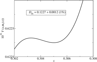
Figure 3: The inflationary potential as a function of the $D3$-position $x$ for the parameters given in (20) and $D_{01}$ modified by $1\%$. The potential is “delicate” since changing the value of $D_{01}$ by $1\%$ modifies the form of the potential from a flat inflection point to one with a local minimum.

This simple one-dimensional fine tuning illustrates the basic problem of the “Delicate Universe.” A more comprehensive scan of the entire parameter space has been carried out in Hoi and Cline (2009), with the conclusion that the set of optimal parameters only needs to be tuned by hand to the level of one part in two. In Section III we will show that this model actually contains a mechanism that can dynamically tune the parameter $D_{01}$ at the level of less than $10\%$, removing the need for the arbitrary fine tuning by hand for this parameter (the other parameters still need to be tuned by hand at the levels discussed in Hoi and Cline (2009), or tuned dynamically by some other mechanism).

II.2 Overshoot Problem

A generic weakness of small field inflation models, and in particular of inflection-point potentials which arise in the model we study here, is that the initial conditions for the inflaton’s position and momentum must be fine tuned in order for inflation to occur. In particular, for an inflection-point potential if the inflaton starts near the inflection point with too large of an initial momentum (or starts at an initial condition high up on the non-slow roll part of the potential) then it will be moving too fast along the flat part of the potential for slow-roll inflation to occur. In order to prevent this overshooting of the inflationary region we must fine tune the initial conditions by hand.

There is a technical complication in studying the overshoot problem for our model concerning the angular coordinates of the mobile D3 brane in the warped throat. As was shown in Baumann et al. (2008), the position of the angular minimum shifts suddenly when the radial coordinate $x$ passes some critical value $x_{c}$. This was determined in Appendix C of Baumann et al. (2008) to be the value at which the quantity $X$ in eq. (C.24) changes sign. We generalize the equation for $X$ to $N_{D3}>1$:

$$X = \pm{2{\cal C}N_{D3}^{1/4}\over n}\frac{(x/\sqrt{N_{D3}})^{3/2}}{\left|1\mp(x/\sqrt{N_{D3}})^{3/2}\right|^{2(1-N_{D3}/n)}}\left\{2\omega+{9\over 2}-\frac{(2\omega_{F}+3)e^{\omega-\omega_{F}}}{\left|1\mp(x/\sqrt{N_{D3}})^{3/2}\right|^{N_{D3}/n}}\right.$$ (21)

$$\left.\mp\frac{3(1-N_{D3}/n)}{\left|1\mp(x/\sqrt{N_{D3}})^{3/2}\right|^{2}}\left[\left({x\over\sqrt{N_{D3}}}\right)^{3/2}\left(1\mp\left({x\over\sqrt{N_{D3}}}\right)^{3/2}\right)-c{x\over\sqrt{N_{D3}}}\right]\right\}.$$

For the model parameters we are primarily interested in (see below), the critical value is close to $x_{c}=1.59$.

Instead of following the detailed motion of the angular brane moduli, we will assume that they quickly move to their new minima since they are heavy. This leads to a sudden drop in the potential, and if this process happened instantaneously, it would make $V(x)$ discontinuous at $x_{c}$. The discontinuity shows up in $V$ through a sign change in various terms in the F-term potential, namely

$$V_{F}(x,\omega) = \frac{a|A_{0}|^{2}}{3U^{2}(x,\omega)}e^{-2\omega}g_{\pm}(\frac{x}{\sqrt{N_{D3}}})^{2N_{D3}/n}$$ (22)

$$\times\left[2\omega+6-2(2\omega_{F}+3)e^{\omega-\omega_{F}}g_{\pm}(\frac{x}{\sqrt{N_{D3}}})^{-N_{D3}/n}\right.$$

$$\left.+\frac{3N_{D3}}{ng_{\pm}(\frac{x}{\sqrt{N_{D3}}})}\left(\frac{cx}{N_{D3}^{1/2}g_{\pm}(\frac{x}{\sqrt{N_{D3}}})}\mp(\frac{x}{N_{D3}^{1/2}})^{3/2}\right)\right]$$

where $g_{\pm}(x)=1\pm(x/\sqrt{N_{D3}})^{3/2}$. To smooth this out, we make the replacement

$$\pm 1\to\tanh(\Lambda(x_{c}-x))$$ (23)

where $\Lambda$ is chosen to be sufficiently large so that the potential for $x<x_{c}$ has reverted to its usual form (14) within a few Hubble times after $x$ passes $x_{c}$. We show the form of the potential for several values in Figure 4. The magnitude of the vertical shift in the potential is relatively small, and it occurs far away from the inflationary region $x\sim 0.06$, where the inflection point is located. We take $\Lambda=100$, which insures that the effects of the transition have damped out within a few e-foldings after $x$ passes $x_{c}$.

    

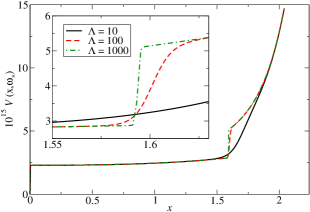
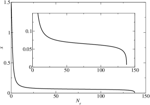
Figure 4: Left: potential with smoothed discontinuity, for smoothing parameter $\Lambda=10,\ 100,\ 1000$ (see eq. (23)). Inset shows close-up of the transition region where angular brane moduli suddenly change. Right: The inflaton $x$ as a function of number of e-foldings. Inset is a close-up of the small-$x$ region where most of inflation occurs.

With this modification we are able to explore the effects of starting high up on the potential, where it is much steeper and the overshoot problem becomes evident. For a given initial field value $x_{\rm init}$ and momentum in the $-x$ direction $v_{\rm init}$ it is straightforward to follow the evolution of the field and determine the total number of e-folds. Since the potential diverges as $x\rightarrow\sqrt{N_{D3}}$ when the $D3$-brane approaches the $D7$-brane, we must restrict the initial field values to $0\leq x\leq\sqrt{N_{D3}}$. In fact one must sometimes be more restrictive, taking $x\leq{\tt min}(\sqrt{N_{D3}},x_{\omega_{*}})$, where $x_{\omega_{*}}$ is the maximum value for which $\partial V/\partial\omega=0$ has a solution, i.e., for which there exists a stable trajectory. To be concrete, let us consider the optimal parameter set (the set of parameters with the smallest amount of overall relative fine tuning) for which the potential has a flat inflection point which supports inflation:

$$D_{01}=0.1995,\quad\omega_{F}=9.761,\quad A_{0}=0.02058,\quad\phi_{\mu}=0.5804,\quad n=8,\quad N_{D3}=5\,.$$ (24)

The allowed initial conditions which lead to $N_{e}\geq 60$ e-folds of inflation are shown as the region below the solid line in Figure 5. For $\phi_{\rm init}/\phi_{\mu}>0.93$, the trajectory is unstable and $\nu_{\rm max}$ is set to zero; for any given initial field value $\phi_{\rm init}/\phi_{\mu}\leq 0.93$ there is always a maximum velocity $v_{\rm init}\leq\nu_{\rm max}(x_{\rm init})$ for which inflation occurs.

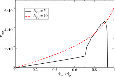
Figure 5: The allowed initial positions $\phi_{\rm init}/\phi_{\mu}$ and velocities $v_{\rm init}$ in the $-x$ direction which give rise to $N_{e}\geq 60$ are in the region below the curves $\nu_{\rm max}$, which is defined as the maximum allowed velocity before overshooting. The solid curve corresponds to the set of parameters (24) which lead to a flat inflection point. The dashed curve corresponds to $N_{D3}=10$ which leads to a local minimum. The trapping of the inflaton by the local minimum occurs for a large range of initial conditions.

Naturally, if the potential has a local minimum rather than an inflection point then we expect that the inflaton will become trapped in the local minimum if it is moving sufficiently slowly. If the inflaton starts with too much initial momentum or too high on the potential, however, then it can still overshoot the local minimum. The region below the dashed line of Figure 5 corresponds to the initial conditions for which the inflaton is trapped in the local minimum of the potential with parameters (24) except with larger $N_{D3}=10$.

One might imagine that the inflaton will overshoot the inflection point if it rolls down the steep part of the potential where the transition happens at $x_{c}$. The solid line in Figure 5, however, belies this expectation, since $x_{c}=1.59$ corresponds to $\phi/\phi_{\mu}=0.71$ by eq. (6), yet we find successful examples of inflation up to $\phi/\phi_{\mu}>0.9$. Figure 6 shows the trajectory of the inflaton starting above the transition point. The inflaton runs into a potential barrier and bounces back to follow the instantaneous minimum trajectory along which inflation occurs. This process damps out a large fraction of the kinetic energy and explains the curious bump in Figure 5. A detailed investigation of the phase space $(\phi,\omega,\dot{\phi},\dot{\omega})$ would be needed for fully understanding the sensitivity to initial conditions, but this is beyond the scope of the present work. Nevertheless, it is clear that the unexpected shift of the instantaneous minimum trajectory implies $v_{\phi}$ is sensitive to the position of $\omega$, and hence inflation becomes more intricate. The case of $N_{D3}=10$, however, is less sensitive since the transition point does not occur in the region $\phi/\phi_{\mu}\leq 1$.

Figure 6: The trajectory (solid line) of the inflaton with initial conditions $\phi_{\rm init}/\phi_{\mu}=0.91$ and $v_{\rm init}=\nu_{\rm max}(\phi_{\rm init})$. The dashed line is the trajectory of the instantaneous minimum; see (8).

II.3 Stabilization of the Kähler Modulus

We conclude this section with a discussion of the stabilization of the Kähler modulus in the scenario with multiple $\overline{D}$-branes and uplifting sectors. One should be concerned that with the addition of many antibranes one introduces a large amount of uplifting energy, which could destabilize the minimum of the Kähler modulus. If the uplifting energy is dominated by other sectors, however,

$$V_{D}(x,\omega)\approx\frac{1}{U^{2}(x,\omega)}\left(D_{1}+2N_{D3}T_{0}\right)\approx\frac{D_{1}}{U^{2}(x,\omega)}\,,$$ (25)

then it is clear that the stabilization of the Kähler modulus is largely independent of the number of antibranes in the inflationary throat since they only enter into the potential through this term. In particular, in Figure 7, we see that the Kähler modulus is not destabilized by the addition of ${\mathcal{O}}(30)$ mobile $D3$-$\overline{D3}$ pairs, as expected.

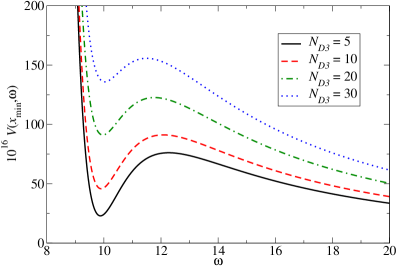
Figure 7: The addition of many mobile D3-branes (stabilized at the local minimum of the potential, $x_{\rm min}$) does not destabilize the Kähler modulus, although it does change the stabilized value.

III Dynamical Fine Tuning in Brane Inflation

In the previous section we identified two fine tuning problems with warped $D$-brane inflation models, the “Delicate Universe” problem of fine tuning in the potential, and the “overshoot problem” of fine tuning in the initial conditions. Both of these problems are present in usual small field inflation as well, but are enhanced due to the inflection-point type potential which occurs in these brane inflation models (as well as in other string-inspired inflationary models Itzhaki and Kovetz (2007); Itzhaki (2008); Linde and Westphal (2008); Conlon et al. (2008); Burgess et al. (2009)). In what follows, we will describe a dynamical mechanism in D-brane inflation models to achieve these required fine tunings.

Let us use a modified set of parameters for our model (exchanging $D_{01}$ for $T_{0}$),

$$\{T_{0},\omega_{F},A_{0},\phi_{\mu}\}$$ effectively continuous (26)

$$\{n,N_{D3}\} \mbox{discrete}\,.$$

Notice that this implies $D_{01}$ is no longer a free parameter, but rather that it depends on the number of $\overline{D}$-branes in the throat,

$$D_{01}=2\frac{N_{D3}T_{0}}{D_{1}}\equiv N_{D3}\Delta D_{01}(\omega_{F},A_{0},n,T_{0})\,,$$ (27)

where we emphasized the fact that $\Delta D_{01}$ is a function of the other parameters. The number of $\overline{D}$-branes in the throat is not constant since $D$-branes can annihilate with $\overline{D}$-branes at the tip of the throat. Keeping all other parameters fixed, removing $D$-branes effectively decreases $D_{01}$ in steps per brane of

$$\Delta D_{01}=2\frac{T_{0}}{D_{1}}\,.$$ (28)

We can then imagine the following scenario: in the pre-inflationary scenario, there are a number of $\overline{D}$- and $D$-branes in the compact space. The $\overline{D}$-branes are quickly attracted to the tip of warped throats by the flux-induced $D3$-charge. The remaining $D$-branes migrate towards the $\overline{D}$-branes, attracted by Coulomb attraction and moduli stabilization effects. All of the parameters (26) are fixed except the number of $D3$-branes $N_{D3}$ which may be large. As a result, the parameter $D_{01}$ in (27) is large, which generically leads to a local minimum in the potential, as shown in the right hand plot of Figure 3. As the $D$-branes fall into the throat (with random initial conditions) they are trapped at the local minimum by two effects: lack of enough energy to overcome the potential barrier, and loss of energy due to open string production by collision with other $D$-branes trapped at the minimum. Gradually, all of the mobile $D$-branes are sitting in a false vacuum of the potential. One by one, the $D$-branes will tunnel out of the false vacuum and annihilate against one of the $\overline{D}$-branes, decreasing the number of $D$-branes in the throat and subsequently decreasing the parameter $D_{01}$ in steps of $\Delta D_{01}$. The tunneling process continues until a sufficiently large number of $D$-branes tunnel out of the local minimum so that $D_{01}^{(n)}=D_{01}-n\Delta D_{01}$ is equal to a critical value at which the local minimum disappears and a flat inflection point appears. The remaining $D$-branes then inflate along this dynamically tuned inflection point. Because all of the remaining $D$-branes are subject to the same force, the stack of branes moves uniformly with the inflaton identified as the radial position of the stack. The schematic picture of this scenario is shown in Figure 2.

In order to remove the necessity to fine-tune by hand the value of $D_{01}$, we would like the step size $\Delta D_{01}$ to be sufficiently small. More precisely, let us consider a fixed set of parameters in (26) (except for $N_{D3}$ of course), let $D_{01}^{*}$ be the value of $D_{01}$ at which a flat inflection point which supports $60$ or more e-folds occurs, and let us say that $D_{01}^{*}$ must be tuned to the level of $1$ part in $1/\delta$ (e.g. to the $\delta\times 100\%$ level). In order to dynamically fine tune the scenario, we need the steps as $D$-branes tunnel from the minimum to be at least equal to the amount of tuning required, e.g. $\delta\geq\Delta D_{01}/D_{01}^{*}$. From (27) this implies that we need at least

$$N_{D3}\geq\delta^{-1}$$ (29)

$D$-branes initially in order to achieve the necessary fine tuning. Clearly, models which require a significant amount of tuning also require a significant number of initial mobile $D$-branes, at which point the probe approximation for the mobile $D$-branes may break down. The point at which the probe approximation breaks down depends on the effective $D3$-charge of the fluxes which generate the warped throat (more precisely, the condition depends on the backreaction of the mobile $D$-branes on the curvature scale of the warped throat), $N_{D3}<N_{\rm eff,D3}$. For typical values up to the bound $N_{\rm eff,D3}\sim{\mathcal{O}}(10^{6})$, we see that we cannot use this mechanism to address severe fine tuning of $D_{01}$ at the level of $1$ part in $10^{6}$ or more. In a later subsection we will actually find that the requirement that the dynamical flattening tunneling process be faster than the timescale for annihilation of the anti-branes with the flux in the throat Kachru et al. (2002) forces the number of antibranes to be small; $N_{D3}\sim{\mathcal{O}}(10)$, corresponding to a dynamical fine tuning at the level of $1$ part in $10$ or so, is a more reasonable expectation (although it may be possible to relax this slightly by allowing different numbers of branes and anti-branes).

III.1 Concrete example

We will now describe a specific set of parameters in which the dynamical mechanism described above does lead to a dynamical scanning of the parameter space ending in a viable inflationary model which matches observational constraints. Suppose that inflation takes place for the optimal parameter values (24), which corresponds to taking the following values for the microscopic parameters:

$$Q_{\mu}=1.07,\ N_{5}=10,\ B_{4}=76.95,\ B_{6}=1.0370$$ (30)

and the corresponding value of $D_{1}$ is $7.260\times 10^{-12}$. This set of parameters requires the same degree of fine tuning as the optimal set shown in ref. Hoi and Cline (2009): $D_{01}$ must be tuned at the 20% level ($\delta D_{01}\cong 0.04$) in order to get successful inflation. To ensure passing through the experimentally allowed interval, the uplifting sources must be chosen such that the increment in $D_{01}$ as branes tunnel from the stack is $\Delta D_{01}\cong 0.04$. Thus with the choice of antibrane tension $T_{0}=1\times 10^{-13}$, which by the relation $T_{0}\sim h_{i}^{4}m_{s}^{4}/g_{s}$ implies that the warp factor at the tip of the throat is approximately $h_{i}\sim 10^{-2}$ (assuming $m_{s}\approx 0.01M_{p}$), we have the step size

$$\Delta D_{01}=2{T_{0}\over D_{1}}=0.04.$$ (31)

Since $D_{01}=N_{D3}\Delta D_{01}$, there must be $N_{D3}=5$ branes in the stack at the time inflation takes place.

For concreteness, imagine starting with $N_{D3}=10$ mobile $D3$-branes, with a corresponding value of $D_{01}=0.3990$. The potential, shown in Figure 8, clearly has a local minimum around $x\approx 0.09$. As the number of $D3$-branes is decreased (corresponding to decreasing $D_{01}$ in steps of $\Delta D_{01}$ (31)), we find that the local minimum disappears and is replaced by an inflection point when the number of mobile $D3$-branes is $N_{D3}=5$, corresponding to the value $D_{01}=0.1995$. Subsequently following the evolution of the two-scalar field system $(x,\omega)$ as in Hoi and Cline (2009), we find an inflationary power spectrum with

$${\mathcal{P}}_{R} = 2.41\times 10^{-9}$$ (32)

$$n_{s} = 0.989$$ (33)

which is within the $2\sigma$ confidence level of the latest WMAP observations.

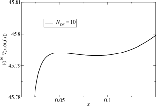
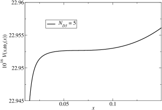
Figure 8: For a large number of mobile D3-branes a local minimum in the inflationary potential exists, trapping the branes at a finite distance in the throat. As individual branes tunnel out of the local minimum, the potential barrier decreases until the local minimum vanishes and is replaced by a very flat inflection point potential. (The height of the potential also goes down with the number of branes.) The tunneling of the branes leads to the dynamical tuning of the parameter $D_{01}$ in small steps.

III.2 Discussion

We have seen an example where the range of values for $D_{01}$ leading to a successful amount of inflation is expanded by our dynamical tunneling mechanism from its naive extent of “by hand” tuning, $\delta D_{01}\cong 0.04$, to a much larger range $\delta D_{01}\cong 0.2$. This is in fact as large as the actual value $D_{01}\cong 0.2$ needed during the final stage after all tunneling events have finished and slow-roll inflation begins; thus the residual fine-tuning problem for this parameter is completely eliminated. It is especially interesting that the mechanism dynamically tunes $D_{01}$, since this is the parameter to which the inflaton potential was found to be most sensitive in Hoi and Cline (2009), for the purpose of getting successful inflation.

Generalizing the above example, we see that in order for this dynamical mechanism to work the change in $D_{01}$ due to tunneling, $\Delta D_{01}$, must be no greater than the naive “by hand” tuning required for successful inflation, $\delta D_{01}$. If this is true, we are guaranteed to pass through the allowed range during some tunneling transition, provided that $D_{01}$ is initially greater than the desired value for inflation. In Figure 9 we show the results of a scan over a large number of models, determining the value of the parameter $D_{01}$ which gives rise to successful inflation and the fractional amount of fine tuning $\delta D_{01}/D_{01}$ of the parameter which is required. It is clear that most of the models require no more tuning than $1$ part in $10$, which can easily be done dynamically with the mechanism presented here, although it is possible that certain individual models may require more tuning than this.

Figure 9: Scatter plot of the fractional amount of required fine tuning $\delta D_{01}/D_{01}$ versus $D_{01}$ for approximately $22,000$ sample inflationary solutions. Most models only require tuning at the level of $1$ part in $10$.

The effective range of allowed values for $D_{01}$ becomes $\Delta N_{D3}\Delta D_{01}$, where $\Delta N_{D3}$ is the number of branes which tunnel between the initial configuration and the final one at which the local minimum disappears and slow-roll inflation begins. This effective range is greater than the naive range of “by hand” tuning by the factor $\Delta N_{D3}\Delta D_{01}/\delta D_{01}$. In the example above, we took $\Delta D_{01}=\delta D_{01}$ and $\Delta N_{D3}=5$ to find an enhancement by a factor of $5$, but it is possible to do even better by taking a larger initial number of branes. This number is only limited by the destabilization of the Kähler modulus and the danger of back-reaction of the branes distorting the background geometry in a way which is not taken into account. For the latter, if the back-reaction effects preserve the existence of a local minimum in the potential the dynamical tunneling regime will still occur, and our mechanism is rather insensitive to the details of the tunneling events as long as normal inflation occurs in the end.

Even if the model parameters do not obey the condition $\Delta D_{01}\leq\delta D_{01}$, we still obtain an enhancement in the range of parameters for which successful inflation can occur, only in this case it is a discrete series of islands in the space of $D_{01}$ rather than a nearly continuous range. As long as $D_{01}$ exceeds the value needed for inflation and $D_{01}/\Delta D_{01}$ is within $\delta D_{01}/\Delta D_{01}$ of being an integer, the last tunneling event will lead to slow roll inflation with the desired properties.

In addition to widening the parameter space compatible with inflation, the space of viable initial conditions for multiple branes is augmented. One effect is that the presence of the local minimum for large numbers of $D3$-branes makes it more difficult to overshoot. Simply comparing the areas below the curves in Figure 5 we see that the local minimum increases the allowed volume of initial conditions leading to $60$ e-folds by a factor of 2. This is actually an underestimate of the effect, since loss of energy through collisions between mobile $D$-branes and other $D$-branes already trapped at the local minimum can be a significant effect Kofman et al. (2004); McAllister and Mitra (2005). We also saw in Figure 6 that in the presence of additional branes the multifield trajectory becomes more intricate, and this can lead to additional helpful features (such as the barrier we saw there) that reduce the overshooting problem. It is clear from this that a more systematic study of the multifield initial conditions space is needed to say more about the tendency of these systems to overshooting, but it also seems that the tendency for overshooting is decreased when the effects of multiple branes are included.

III.3 Tunneling Rate

In the scenario as we have so far described it, the inflationary brane stack can sit in the metastable local minimum for an arbitrary amount of time before the final tunneling which initiates normal slow-roll inflation. However, there is a competing tunneling process which could in principle interfere with this picture, namely the annihilation of the $\overline{D}$-branes at the tip of the throat with the background flux, as described in ref. Kachru et al. (2002) (KPV). We need to make sure that the branes in our stack have time to tunnel before this geometry-changing transition can take place. To this end, we estimate the rates for the two processes in the present section.

First, let us estimate the rate for $D$-branes to tunnel from the local minimum. We note that the potential does not flatten out immediately after a $D$-brane tunnels, but rather it only flattens once the $D$-brane classically rolls to the tip of the throat and annihilates with an $\overline{D}$-brane. This means that there is no energy benefit for multiple branes to tunnel at once, so that the rate for $n$ branes to tunnel is the $n$th power of the tunneling rate for one brane; thus single brane tunneling is most likely. Further, because the tunneling timescale is long, any velocity-dependent interactions between the branes, such as open-string creation, are suppressed as well, and we can use a single field description for tunneling.

There are several different estimates of the tunneling rate, depending on the features of the potential. The rate for standard Coleman-De Luccia (CDL) instantons depends on whether there is significant gravitational backreaction Coleman and De Luccia (1980),

$$\Gamma_{CDL}\sim\cases{\mbox{exp}\left(-\frac{27\pi^{2}}{2}\frac{T^{4}}{V_{\rm min}^{3}}\right),&w/o\, gravitational back-reaction ($M_{p}^{2}V_{\rm min}\gg T^{2}$)\cr\mbox{exp}\left(-\frac{24\pi^{2}}{V_{\rm min}}\right),&with gravitational back-reaction ($M_{p}^{2}V_{\rm min}\ll T^{2}$)\,,\cr}$$ (34)

where $V_{\rm min}$ is the vacuum energy in the false vacuum, and the tension of the bubble of true vacuum

$$T=\int d\phi\sqrt{2V(\phi)}\sim\sqrt{V_{\rm max}}\Delta\phi$$ (35)

depends on the height $V_{\rm max}$ and width $\Delta\phi$ of the potential barrier. Alternatively, Hawking-Moss instantons depend only upon the separation between the false vacuum and the maximum of the potential barrier Hawking and Moss (1982),

$$\Gamma_{HM}\sim\mbox{exp}\left(-24\pi^{2}\left(\frac{M_{p}^{4}}{V_{\rm min}}-\frac{M_{p}^{4}}{V_{\rm max}}\right)\right)\,.$$ (36)

In the dynamical fine tuning scenario outlined above, the height of the potential barrier is small and decreases with each successive tunneling event, so we have $V_{\rm max}=V_{\rm min}(1+\epsilon)$ for some $\epsilon\ll 1$. We can ignore gravitational backreaction in the CDL instanton estimate since

$$\frac{T^{2}}{M_{p}^{2}V_{\rm min}}\sim\frac{\Delta\phi^{2}}{M_{p}^{2}}\frac{V_{\rm max}}{V_{\rm min}}\sim\frac{\Delta\phi^{2}}{M_{p}^{2}}\ll 1\,,$$ (37)

where in the last step we used that $\Delta\phi/M_{p}\ll 1$ for warped brane inflation models Chen et al. (2006); Baumann and McAllister (2007). The decay rate for branes to tunnel from the local minimum through the dynamical fine tuning process is then

$$\Gamma_{\rm dyn}\sim\mbox{exp}\left(-24\pi^{2}\frac{\alpha M_{p}^{4}}{V_{\rm min}}\right),$$ (38)

where $\alpha$ is the smaller of $\{\frac{9}{16}\frac{\Delta\phi^{4}}{M_{p}^{4}},\epsilon\}\ll 1$. For typical shapes of the potential we have $\Delta\phi^{4}/M_{p}^{4}\ll\epsilon$, so the decay rate is dominated by the CDL instanton.

Next we turn to the other relevant quantum tunneling process for this scenario, that of the annihilation of the $\overline{D3}$-branes with the flux in the throat, as described by Kachru, Pearson and Verlinde (KPV) Kachru et al. (2002) and studied in greater detail in the references Frey et al. (2003); Freivogel and Lippert (2008); Brown and DeWolfe (2009). With $M$ units of $F_{3}$ flux wrapped on the $A$-cycle of the throat and $K$ units of $H_{3}$ flux wrapped on the $B$-cycle of the throat we have an effective $D3$-charge of $N_{\rm eff}=MK$ and a warp factor of $h_{A}\sim e^{-2\pi K/(3g_{s}M)}$. When there are $p$ $\overline{D3}$-branes at the tip of the throat with $p/M\geq 0.08$, the configuration is classically unstable against the $\overline{D}$-branes annihilating with the fluxes. Since we have the same number of branes and antibranes, this puts another limit on the number of $D$-branes we can have in our compactification, $N_{D3}\leq 0.08\times N_{\rm eff,D3}/K$ which is somewhat more stringent than the one derived before due to backreaction. We will assume that we have large enough flux $M$ so that this effect can only proceed via quantum decay through CDL instantons. The rate, including corrections found in Freivogel and Lippert (2008), is

$$\Gamma_{KPV}\sim\mbox{exp}\left(-\beta\,{g_{s}M^{6}\over N_{\overline{D3}}^{3}}\right)\,,$$ (39)

where $\beta=3\times 10^{-3}$ is a pure number fixed for the geometry. Demanding that this be slower than the brane-tunneling rate (38) gives us a restriction on the $F_{3}$ flux,

$$M>\left(\frac{27\pi^{2}}{2\beta}\right)^{1/6}\frac{\Delta x^{2/3}\phi_{\mu}^{2/3}N_{D3}^{1/2}}{g_{s}^{1/6}V_{\rm min}^{1/6}}$$ (40)

(where we have again used our simplifying assumption that $N_{\overline{D3}}=N_{{D3}}$). Using the definition $\phi_{\mu}/M_{p}\equiv\frac{2}{\sqrt{MK}}\frac{1}{Q_{\mu}\sqrt{B_{6}}}<\frac{2}{\sqrt{MK}}$ where $Q_{\mu},B_{6}\geq 1$ and the definition of the vacuum energy in the local minimum $V_{\rm min}=\frac{2N_{D3}h_{A}^{4}}{(2\pi)^{3}g_{s}\ell_{s}^{4}}$ in terms of the fluxes $h_{A}=e^{-2\pi K/(3g_{s}M)}$, we can turn the requirement that KPV tunneling be suppressed into a bound on the parameter $\phi_{\mu}$,

$$\phi_{\mu}<\phi_{\rm max}\equiv 2^{3/5}\left(\frac{8\pi}{3}\right)^{3/10}\left(\frac{2\beta}{27\pi^{2}}\right)^{1/10}\frac{(V_{\rm min}/M_{p}^{4})^{1/10}}{g_{s}^{1/5}\,\Delta x^{2/5}\,N_{D3}^{3/10}\left(\ln\frac{2N_{D3}}{(2\pi)^{3}V_{\rm min}g_{s}\ell_{s}^{4}}\right)^{3/10}}\,.$$ (41)

When this bound is satisfied, KPV tunneling will be suppressed relative to the dynamical tuning effect. Surprisingly, this bound is difficult to satisfy—for the “optimal” parameter set presented in (24) with

$$V_{\rm min}\cong(2.6\times 10^{-4})^{4},\,\Delta x\cong 0.05,\,N_{D3}\cong 10,\,g_{s}\cong 0.1,\,\ell_{s}\cong 0.1,$$

we have $\phi_{\rm max}\approx 0.025$, which is much smaller than the value of the parameter $\phi_{\mu}=0.5804$. One way to satisfy the bound is to adjust $\phi_{\rm max}$ by reducing the value of $g_{s}$; however, since the bound (41) is only sensitive to $g_{s}^{1/5}$ we need to reduce the string coupling by a large factor to $g_{s}\sim 10^{-8}$. This allows the bound to be satisfied $\phi_{\rm max}\approx 0.70>\phi_{\mu}$ and leads to the tunneling rates

$$\Gamma_{\rm dyn} \sim e^{-2\times 10^{10}}$$

$$\Gamma_{KPV} \sim e^{-9\times 10^{10}}$$

which indicate that the dynamical fine tuning effect indeed dominates.

It is possible that there exists a parameter regime where the dominance of dynamical flattening over KPV tunneling can be achieved with a more realistic value of the string coupling (e.g. $g_{s}\sim 0.01$). In particular, instead of attempting to make the value of $\phi_{\rm max}$ in the bound larger by suppressing $g_{s}$, one can search for inflationary models with small $\phi_{\mu}$. Based on the observation that there is a degeneracy between $\phi_{\mu}$ and the number of D7-branes $n$ Hoi and Cline (2009), we have done some simple numerical searches of the parameter space and find that most models seem to require an equally unrealistic number of D7-branes $n\sim 10^{3}$, although we have not done a complete scan of parameter space. Since models which allow dynamical fine tuning to dominate the decay rate do not seem to be generic in parameter space, this raises the open question as to how much the dynamical effect will help the overall fine tuning required to obtain a viable model.

IV Conclusion

The idea that our universe could have emerged from a series of tunneling events has become rather popular in the context of the string theory landscape of vacua. In this paper, we have provided an explicit open-string example of this idea within the warped brane-antibrane inflation model, where branes from a stack trapped in the throat sequentially tunnel through a potential barrier to the bottom of the throat. The remarkable feature here is that it can be natural for the final tunneling event to lead to slow roll inflation, because the barrier becomes increasingly shallow after each tunneling. The concept of naturalness is quantified by the range of values of the parameter $D_{01}=D_{0}/D_{1}$ which (together with appropriate values of other parameters) are compatible with the CMB power spectrum observed in our universe. (The parameter $D_{01}$ is the ratio of uplifting due to antibranes in the inflationary throat versus that coming from other sources, such as other throats.) The range which leads to successful inflation after tunneling depends on how many branes tunnel, and could be enhanced relative to the usual value by a factor of 100 or even 1000, limited only by the number of branes which can be trapped in the throat before their back-reaction seriously alters the background throat geometry, or destabilization of the Kähler modulus from its dS vacuum.

Not only can successful inflation result from a much larger range of parameters of the model than previously thought, but also the range of initial conditions is expanded. This is because the problem of the inflaton overshooting the inflection point, where inflation should take place, is ameliorated if the inflection point is initially replaced by a local minimum of the potential. Once the stack of branes is trapped at the minimum, it will naturally start rolling away from the flattest region of the potential with initially vanishing velocity. This occurs at the moment of the final tunneling event when the last shallow local minimum converts to a monotonic potential, which is close to having an inflection point.

In order for the dynamical tunneling process to be faster than other decay processes, such as $\overline{D3}$-branes annihilating with the flux at the tip of the throat as in KPV Kachru et al. (2002), we found we needed to tune the string coupling to be quite small, although other parameter regimes without such extreme tuning of the string coupling may exist. It remains to be seen how generic this picture of a dynamical open string inflationary landscape is within the full set of allowed parameters.

References

- Dvali and Tye (1999) G. R. Dvali and S. H. H. Tye, Phys. Lett. B450, 72 (1999), eprint hep-ph/9812483.
- Kachru et al. (2003) S. Kachru et al., JCAP 0310, 013 (2003), eprint hep-th/0308055.
- Baumann et al. (2006) D. Baumann et al., JHEP 11, 031 (2006), eprint hep-th/0607050.
- Burgess et al. (2007) C. P. Burgess, J. M. Cline, K. Dasgupta, and H. Firouzjahi, JHEP 03, 027 (2007), eprint hep-th/0610320.
- Baumann et al. (2008) D. Baumann, A. Dymarsky, I. R. Klebanov, and L. McAllister, JCAP 0801, 024 (2008), eprint 0706.0360.
- Krause and Pajer (2008) A. Krause and E. Pajer, JCAP 0807, 023 (2008), eprint 0705.4682.
- Panda et al. (2007) S. Panda, M. Sami, and S. Tsujikawa, Phys. Rev. D76, 103512 (2007), eprint 0707.2848.
- Ali et al. (2009) A. Ali, R. Chingangbam, S. Panda, and M. Sami, Phys. Lett. B674, 131 (2009), eprint 0809.4941.
- Baumann et al. (2009) D. Baumann, A. Dymarsky, S. Kachru, I. R. Klebanov, and L. McAllister, JHEP 03, 093 (2009), eprint 0808.2811.
- Linde and Westphal (2008) A. Linde and A. Westphal, JCAP 0803, 005 (2008), eprint 0712.1610.
- Itzhaki and Kovetz (2007) N. Itzhaki and E. D. Kovetz, JHEP 10, 054 (2007), eprint 0708.2798.
- Underwood (2008) B. Underwood, Phys. Rev. D78, 023509 (2008), eprint 0802.2117.
- Itzhaki (2008) N. Itzhaki, JHEP 10, 061 (2008), eprint 0807.3216.
- Hoi and Cline (2009) L. Hoi and J. M. Cline, Phys. Rev. D79, 083537 (2009), eprint 0810.1303.
- Cline and Stoica (2005) J. M. Cline and H. Stoica, Phys. Rev. D72, 126004 (2005), eprint hep-th/0508029.
- Kofman et al. (2004) L. Kofman et al., JHEP 05, 030 (2004), eprint hep-th/0403001.
- McAllister and Mitra (2005) L. McAllister and I. Mitra, JHEP 02, 019 (2005), eprint hep-th/0408085.
- Barnaby et al. (2005) N. Barnaby, C. P. Burgess, and J. M. Cline, JCAP 0504, 007 (2005), eprint hep-th/0412040.
- Chialva et al. (2006) D. Chialva, G. Shiu, and B. Underwood, JHEP 01, 014 (2006), eprint hep-th/0508229.
- Kofman and Yi (2005) L. Kofman and P. Yi, Phys. Rev. D72, 106001 (2005), eprint hep-th/0507257.
- Chen and Tye (2006) X. Chen and S. H. H. Tye, JCAP 0606, 011 (2006), eprint hep-th/0602136.
- Berndsen et al. (2008) A. Berndsen, J. M. Cline, and H. Stoica, Phys. Rev. D77, 123522 (2008), eprint 0710.1299.
- Klebanov and Strassler (2000) I. R. Klebanov and M. J. Strassler, JHEP 08, 052 (2000), eprint hep-th/0007191.
- Giddings et al. (2002) S. B. Giddings, S. Kachru, and J. Polchinski, Phys. Rev. D66, 106006 (2002), eprint hep-th/0105097.
- Burgess et al. (2003) C. P. Burgess, R. Kallosh, and F. Quevedo, JHEP 10, 056 (2003), eprint hep-th/0309187.
- Jockers and Louis (2005) H. Jockers and J. Louis, Nucl. Phys. B718, 203 (2005), eprint hep-th/0502059.
- Cremades et al. (2007) D. Cremades, M. P. Garcia del Moral, F. Quevedo, and K. Suruliz, JHEP 05, 100 (2007), eprint hep-th/0701154.
- Chen and Gong (2008) H.-Y. Chen and J.-O. Gong (2008), eprint 0812.4649.
- DeWolfe and Giddings (2003) O. DeWolfe and S. B. Giddings, Phys. Rev. D67, 066008 (2003), eprint hep-th/0208123.
- Giddings and Maharana (2006) S. B. Giddings and A. Maharana, Phys. Rev. D73, 126003 (2006), eprint hep-th/0507158.
- Shiu et al. (2008) G. Shiu, G. Torroba, B. Underwood, and M. R. Douglas, JHEP 06, 024 (2008), eprint 0803.3068.
- Douglas and Torroba (2008) M. R. Douglas and G. Torroba (2008), eprint 0805.3700.
- Frey et al. (2009) A. R. Frey, G. Torroba, B. Underwood, and M. R. Douglas, JHEP 01, 036 (2009), eprint 0810.5768.
- Gukov et al. (2000) S. Gukov, C. Vafa, and E. Witten, Nucl. Phys. B584, 69 (2000), eprint hep-th/9906070.
- Kuperstein (2005) S. Kuperstein, JHEP 03, 014 (2005), eprint hep-th/0411097.
- Huang et al. (2008) M.-x. Huang, G. Shiu, and B. Underwood, Phys. Rev. D77, 023511 (2008), eprint 0709.3299.
- Langlois et al. (2008a) D. Langlois, S. Renaux-Petel, D. A. Steer, and T. Tanaka, Phys. Rev. Lett. 101, 061301 (2008a), eprint 0804.3139.
- Langlois et al. (2008b) D. Langlois, S. Renaux-Petel, D. A. Steer, and T. Tanaka, Phys. Rev. D78, 063523 (2008b), eprint 0806.0336.
- Chen et al. (2008) H.-Y. Chen, J.-O. Gong, and G. Shiu, JHEP 09, 011 (2008), eprint 0807.1927.
- Conlon et al. (2008) J. P. Conlon, R. Kallosh, A. Linde, and F. Quevedo, JCAP 0809, 011 (2008), eprint 0806.0809.
- Burgess et al. (2009) C. P. Burgess, J. M. Cline, and M. Postma, JHEP 03, 058 (2009), eprint 0811.1503.
- Kachru et al. (2002) S. Kachru, J. Pearson, and H. L. Verlinde, JHEP 06, 021 (2002), eprint hep-th/0112197.
- Coleman and De Luccia (1980) S. R. Coleman and F. De Luccia, Phys. Rev. D21, 3305 (1980).
- Hawking and Moss (1982) S. W. Hawking and I. G. Moss, Phys. Lett. B110, 35 (1982).
- Chen et al. (2006) X. Chen, S. Sarangi, S. H. Henry Tye, and J. Xu, JCAP 0611, 015 (2006), eprint hep-th/0608082.
- Baumann and McAllister (2007) D. Baumann and L. McAllister, Phys. Rev. D75, 123508 (2007), eprint hep-th/0610285.
- Frey et al. (2003) A. R. Frey, M. Lippert, and B. Williams, Phys. Rev. D68, 046008 (2003), eprint hep-th/0305018.
- Freivogel and Lippert (2008) B. Freivogel and M. Lippert, JHEP 12, 096 (2008), eprint 0807.1104.
- Brown and DeWolfe (2009) C. M. Brown and O. DeWolfe, JHEP 05, 018 (2009), eprint 0901.4401.