Dromion solutions of noncommutative Davey-Stewartson equations

Abstract

We consider a noncommutative version of the Davey-Stewartson equations and derive two families of quasideterminant solution via Darboux and binary Darboux transformations. These solutions can be verified by direct substitution. We then calculate the dromion solutions of the equations and obtain computer plots in a noncommutative setting.

1 Introduction

The Davey-Stewartson (DS) equations have become a topic of much interest in recent years. Derived by A. Davey and K. Stewartson in $1974$ [4], the system is nonlinear in $(2+1)$-dimensions and describes the evolution of a three-dimensional wave-packet on water of finite depth. By carrying out a suitable dimensional reduction, the system can be reduced to the $(1+1)$-dimensional nonlinear Schrödinger (NLS) equation.
A major development in the understanding of the DS equations came in $1988$, when Boiti et al. [3] discovered a class of exponentially localised solutions (two-dimensional solitons) which undergo a phase shift and possible amplitude change on interaction with other solitons. These were later termed dromions by Fokas and Santini [6], derived from the Greek dromos meaning tracks, to highlight that the dromions lie at the intersection of perpendicular track-like plane waves.
Multidromion solutions to the DS system have been obtained using a variety of approaches - the inverse scattering method [6], Hirota’s direct method [13] and others. These solutions have been determined both in terms of Wronskian [13] and Grammian [10] determinants.
Additionally, there has been considerable interest in noncommutative versions of the DS equations. Hamanaka [12] derived a system with noncommutativity defined in terms of the Moyal star product [19], while more recently, Dimakis and Müller-Hoissen [5] determined a similar system from a multicomponent KP hierarchy. This then enabled calculation of dromion solutions in the matrix case.
The strategy that we employ here, whereby we introduce noncommutativity into an integrable nonlinear wave equation without destroying the solvability, has previously been considered by others in the field, for example by Lechtenfeld and Popov [16], and by Lechtenfeld, Popov et al in [15], where a noncommutative version of the sine-Gordon equation is discussed.
In this paper we are not concerned with the nature of the noncommutativity, and derive a system of noncommutative DS equations in the most general way by utilising the same Lax pair as in the commutative case but assuming no commutativity of the dependent variables. This method has also been employed by Gilson and Nimmo in [11] for the case of the noncommutative Kadomtsev-Petviashvili (KP) equation. We find that the noncommutative DS system obtained in this manner corresponds to that given in an earlier paper by Schultz, Ablowitz and Bar Yaacov [21], where a quantum version of the DS equation is ultimately discussed.
We derive quasiwronskian and quasigrammian solutions of this system in section 4 via Darboux and binary Darboux transformations and, in section 6, verify these solutions by direct substitution.
We then use the quasigrammian solution to determine a class of dromion solution and, by specifying that certain parameters in the solution are of matrix rather than scalar form, obtain dromion solutions in the noncommutative case. We conclude with computer plots of these dromion solutions.

2 Noncommutative Davey-Stewartson equations

We consider the system of commutative DS equations given by Ablowitz and Schultz in [2], with Lax pair

$$L =\partial_{x}-\varLambda+\sigma{J}\partial_{y},$$ (2.1a)

$$M =\partial_{t}-A+\frac{\textrm{i}}{\sigma}\varLambda\partial_{y}-\textrm{i}J\partial_{yy},$$ (2.1b)

where

$$J=\begin{pmatrix}1&0\\ 0&-1\end{pmatrix},\,\varLambda=\begin{pmatrix}0&q(x,y,t)\\ r(x,y,t)&0\end{pmatrix}$$ (2.2)

for $r=\pm{q}^{*}$ ($q^{*}$ denotes the complex conjugate of $q$) and $A$ is a $2\times{2}$ matrix given by

$$A=\begin{pmatrix}A_{1}&\displaystyle\frac{\textrm{i}}{2\sigma^{2}}(q_{x}-\sigma{q}_{y})\\ -\displaystyle\frac{\textrm{i}}{2\sigma^{2}}(r_{x}+\sigma{r}_{y})&A_{2}\end{pmatrix}.$$ (2.3)

We choose $\sigma=-1$ or $\sigma=\textrm{i}$ for the DSI and DSII equations respectively. By considering the same Lax pair (2.1a,b) as is used in the commutative case and assuming no commutativity of variables (we do not specify the nature of the noncommutativity), we obtain the compatibility condition

$$-A_{x}+[\varLambda,A]+\varLambda_{t}-\sigma{J}A_{y}+\frac{\textrm{i}}{\sigma}\varLambda\varLambda_{y}-\textrm{i}J\varLambda_{yy} =0,$$ (2.4a)

$$\frac{\textrm{i}}{\sigma}\varLambda_{x}+\sigma[A,J]-\textrm{i}J\varLambda_{y} =0,$$ (2.4b)

from which we generate a system of noncommutative Davey-Stewartson (ncDS) eqations

$$\textrm{i}q_{t} =-\frac{1}{2\sigma^{2}}\left(q_{xx}+\sigma^{2}q_{yy}\right)+\textrm{i}(A_{1}q-qA_{2}),$$ (2.5a)

$$\textrm{i}r_{t} =\frac{1}{2\sigma^{2}}\left(r_{xx}+\sigma^{2}r_{yy}\right)-\textrm{i}(rA_{1}-A_{2}r),$$ (2.5b)

$$(\partial_{x}+\sigma\partial_{y})A_{1} =-\frac{\textrm{i}}{2\sigma^{2}}(\partial_{x}-\sigma\partial_{y})(qr),$$ (2.5c)

$$(\partial_{x}-\sigma\partial_{y})A_{2} =\frac{\textrm{i}}{2\sigma^{2}}(\partial_{x}+\sigma\partial_{y})(rq).$$ (2.5d)

(Note that we obtain from the above system the nonlinear Schrödinger (NLS) equation [1]

$$\textrm{i}{q_{t}+q_{yy}\pm{2}qrq=0}$$ (2.6)

and its corresponding complex conjugate by taking a dimensional reduction $\partial_{x}=0$, with $A_{1}=\pm{\frac{\textrm{i}}{2}}qr,$ $A_{2}=\pm\frac{\textrm{i}}{2}rq$ [12]).
 
 For notational convenience, and to avoid the use of identities later when verifying solutions, we introduce a $2\times{2}$ matrix $S=(s_{ij})$ ($i,j=1,2$) such that $\varLambda=[J,\sigma{S}]$ [17], and hence

$$S=\begin{pmatrix}s_{11}&\displaystyle\frac{q}{2\sigma}\\ -\displaystyle\frac{r}{2\sigma}&s_{22}\end{pmatrix}.$$ (2.7)

Additionally, by setting

$$A=\frac{\textrm{i}}{\sigma}S_{x}-\textrm{i}JS_{y},$$ (2.8)

equation (2.4b) is automatically satisfied, and (2.4a) becomes

$$-\frac{\textrm{i}}{\sigma}S_{xx}+\textrm{i}JSS_{x}-\textrm{i}SJS_{x}-\textrm{i}S_{x}JS+\textrm{i}S_{x}SJ+\textrm{i}\sigma{J}S_{y}JS\\ -\textrm{i}\sigma{J}S_{y}SJ+\sigma{J}S_{t}-\sigma{S}_{t}J-\textrm{i}\sigma{J}SS_{y}J+\textrm{i}\sigma{S}JS_{y}J+\textrm{i}\sigma{J}S_{yy}J=0.$$ (2.9)

Note that this is essentially the noncommutative analogue of the Hirota bilinear form (see for example [14]) of the DS equations.

3 Quasideterminants

Here we briefly recall some of the properties of quasideterminants. A more detailed analysis can be found in the original papers [8, 9].
The notion of a quasideterminant was first introduced by Gelfand and Retakh in [9] as a straightforward way to define the determinant of a matrix with noncommutative entries. Many equivalent definitions of quasideterminants exist, one such being a recursive definition involving inverse minors. Let $A=(a_{ij})$ be an $n\times{n}$ matrix with entries over a usually noncommutative ring $\mathcal{R}$. We denote the $(i,j)^{\text{th}}$ quasideterminant by $\mid\!{A}\!\mid_{ij}$, where

$$\mid\!{A}\!\mid_{ij}\,=a_{ij}-r_{i}^{j}(A^{ij})^{-1}s_{j}^{i}.$$ (3.1)

Here, $A^{ij}$ is the $(n-1)\times(n-1)$ minor matrix obtained from $A$ by deleting the $i^{\text{th}}$ row and the $j^{\text{th}}$ column (note that this matrix must be invertible), $r_{i}^{j}$ is the row vector obtained from the $i^{\text{th}}$ row of $A$ by deleting the $j^{\text{th}}$ entry, and $s_{j}^{i}$ is the column vector obtained from the $j^{\text{th}}$ column of $A$ by deleting the $i^{\text{th}}$ entry.
A common notation employed when discussing quasideterminants is to ‘box’ the expansion element, i.e. we write

$$\mid\!A\!\mid_{11}=\begin{vmatrix}\boxed{a_{11}}&a_{12}\\ a_{21}&a_{22}\end{vmatrix}$$ (3.2)

to denote the $(1,1)^{\textrm{th}}$ quasideterminant. It should be noted that the above expansion formula is also valid in the case of block matrices, provided the matrix to be inverted is square; for example considering a block matrix

$$\begin{pmatrix}N&B\\ C&d\end{pmatrix},$$

where $N$ is a square matrix over $\mathcal{R}$, $B$ and $C$ are column and row vectors over $\mathcal{R}$ of compatible lengths, and $d\in\mathcal{R}$, we have

$$\begin{vmatrix}N&B\\ C&\boxed{d}\end{vmatrix}=d-CN^{-1}B.$$ (3.3)

Quasideterminants also provide a useful formula for the inverse of a matrix: for an invertible $n\times{n}$ matrix $A=(a_{ij})\,(i,j=1,\ldots,n)$, the $(i,j)^{\textrm{th}}$ entry of $A^{-1}$ is given by

$$(A^{-1})_{ij}=\bigl{(}\mid\!A\!\mid_{ji}\bigr{)}^{-1}.$$ (3.4)

When the elements of $A$ commute, the quasideterminant $\mid\!A\!\mid_{ij}$ is not simply the determinant of $A$, but rather a ratio of determinants: it is well-known that, for $A$ invertible, the $(j,i)^{\text{th}}$ entry of $A^{-1}$ is

$$(-1)^{i+j}\frac{\det{A^{ij}}}{\det{A}}.$$

Then, by (3.4), we can easily see that

$$\mid\!A\!\mid_{ij}=(-1)^{i+j}\frac{\det{A}}{\det{A^{ij}}}$$ (3.5)

in the commutative case.

4 Quasideterminant solutions via Darboux transformations

4.1 Darboux transformations

Here we give a brief overview of Darboux transformations. Further information can be found in, for example, [18].
We follow the notation given in [11]. Let $\theta_{1},\ldots,\theta_{n}$ be a particular set of eigenfunctions of an operator $L$, and define $\Theta=(\theta_{1},\ldots,\theta_{n})$ and $\widehat{\Theta}=\Bigl{(}\theta_{j}^{(i-1)}\Bigr{)}$ for $i,j=1,\ldots,n$, the $n\times{n}$ Wronskian matrix of $\theta_{1},\ldots,\theta_{n}$, where ^(k) denotes the $k^{\textrm{th}}$ $y$-derivative.
To iterate the Darboux transformation, let $\theta_{[1]}=\theta_{1}$ and $\phi_{[1]}=\phi$ be a general eigenfunction of $L_{[1]}=L$, with $L_{[1]}$ covariant under the action of the Darboux transformation $G_{\theta_{[1]}}=\partial_{y}-\theta_{[1]}^{(1)}\theta_{[1]}^{-1}$. Then the general eigenfunctions $\phi_{[2]}$ for $L_{[2]}=G_{\theta_{[1]}}L_{[1]}G_{\theta_{[1]}}^{-1}$ are given by

$$\phi_{[2]}=G_{\theta_{[1]}}\bigl{(}\phi_{[1]}\bigr{)}=\phi_{[1]}^{(1)}-\theta_{[1]}^{(1)}\theta_{[1]}^{-1}\phi_{[1]},$$ (4.1)

with

$$\theta_{[2]}=\phi_{[2]}|_{\phi\rightarrow\theta_{2}.}$$ (4.2)

Continuing this process, after $n$ iterations ($n\geq{1}),$ the $n^{\textrm{th}}$ Darboux transformation of $\phi$ is given by

$$\phi_{[n+1]}=\phi_{[n]}^{(1)}-\theta_{[n]}^{(1)}\theta_{[n]}^{-1}\phi_{[n]},$$ (4.3)

where

$$\theta_{[k]}=\phi_{[k]}|_{\phi\rightarrow\theta_{k}}.$$ (4.4)

4.2 Quasiwronskian solution of ncDS using Darboux transformations

We now determine the effect of the Darboux transformation $G_{\theta}=\partial_{y}-\theta_{y}\theta^{-1}$ on the Lax operator $L$ given by (2.1a), with $\theta$ an eigenfunction of $L$. Corresponding results hold for the operator $M$ given by (2.1b). $L$ is covariant with respect to the Darboux transformation, and, by supposing that $L$ is transformed to a new operator $\tilde{L}$, say, we calculate that the effect of the Darboux transformation $\tilde{L}=G_{\theta}LG_{\theta}^{-1}$ is such that

$$\tilde{\varLambda}=\varLambda-\sigma[J,\theta_{y}\theta^{-1}].$$ (4.5)

Recalling that $\varLambda=[J,\sigma{S}]$, we have $\tilde{S}=S-\theta_{y}\theta^{-1}$, and hence, after $n$ repeated Darboux transformations,

$$S_{[n+1]}=S_{[n]}-(\theta_{[n]})_{y}\theta_{[n]}^{-1},$$ (4.6)

where $S_{[1]}=S$, $\theta_{[1]}=\theta$. We express $S_{[n+1]}$ in quasideterminant form as

$$S_{[n+1]} =S+\begin{vmatrix}\theta_{1}&\ldots&\theta_{n}&\begin{array}[]{cc}0&0\\ 0&0\end{array}\\ \vdots&{}&\vdots&\vdots\\ \theta_{1}^{(n-2)}&\ldots&\theta_{n}^{(n-2)}&\begin{array}[]{cc}0&0\\ 0&0\end{array}\\ \theta_{1}^{(n-1)}&\ldots&\theta_{n}^{(n-1)}&\begin{array}[]{cc}1&0\\ 0&1\end{array}\\ \theta_{1}^{(n)}&\ldots&\theta_{n}^{(n)}&\boxed{\begin{array}[]{cc}0&0\\ 0&0\end{array}}\end{vmatrix},$$ (4.7)

where ^(k) denotes the $k^{\textrm{th}}$ $y$-derivative. It should be noted here that each $\theta_{i}$ ($i=1,\ldots,n$) is not a single entry but a $2\times{2}$ matrix (since the $\theta_{i}$ are eigenfunctions of $L,M$). The Wronskian-like quasideterminant in (4.7) is termed a quasiwronskian, see [11], and [7] for details of Wronskian determinants.
For ease of notation, for integers $i,j=1,\ldots,n$, we denote by $Q(i,j)$ the quasideterminant [11]

$$Q(i,j)=\begin{vmatrix}\widehat{\Theta}&\begin{array}[]{cc}f_{j}&e_{j}\end{array}\\ \Theta^{(n+i)}&\boxed{\begin{array}[]{cc}0&0\\ 0&0\end{array}}\end{vmatrix},$$ (4.8)

where, as before, $\widehat{\Theta}=(\theta_{j}^{(i-1)})_{i,j=1,\ldots,n}$ is the $n\times{n}$ Wronskian matrix of $\theta_{1},\ldots,\theta_{n}$ and ^(k) denotes the $k^{\textrm{th}}$ $y$-derivative, $\Theta$ is the row vector $\left(\theta_{1},\ldots,\theta_{n}\right)$ of length $n$, and $f_{j}$ and $e_{j}$ are $2n\times{1}$ column vectors with a $1$ in the $(2n-2j-1)^{\textrm{th}}$ and $(2n-2j)^{\textrm{th}}$ row respectively and zeros elsewhere. Again each $\theta_{i}$ is a $2\times{2}$ matrix. In this definition of $Q(i,j)$, we allow $i,j$ to take any integer values subject to the convention that if either $2n-2j$ or $2n-2j-1$ lies outside the range $1,2,\ldots,2n$, then $e_{j}=f_{j}=0$ and so $Q(i,j)=0$. Hence (4.7) can be written as

$$S=S_{0}+Q(0,0),$$ (4.9)

where $S_{0}$ is any given solution of the ncDS equations. Here we choose the vacuum solution $S_{0}=0$ for simplicity.
It will be useful to express the quasiwronskian solution (4.9) in terms of the variables $q$ and $r$, the variables in which the ncDS equations (2.5a-d) are expressed. We have

$$S=Q(0,0),$$ (4.10)

which gives, by applying the quasideterminant expansion formula (3.1) and expressing each $\theta_{i}$ ($i=1,\ldots,n$) as an appropriate $2\times{2}$ matrix

$$\theta_{i}=\begin{pmatrix}\phi_{2i-1}&\phi_{2i}\\ \psi_{2i-1}&\psi_{2i}\end{pmatrix}$$ (4.11)

for $\phi=\phi(x,y,t),\,\psi=\psi(x,y,t)$, an expression for $S$ in terms of quasiwronskians, namely

$$S=\begin{pmatrix}\begin{vmatrix}\widehat{\Theta}&f_{0}\\ \phi^{(n)}&\boxed{0}\end{vmatrix}&\begin{vmatrix}\widehat{\Theta}&e_{0}\\ \phi^{(n)}&\boxed{0}\end{vmatrix}\\ {}&{}\\ \begin{vmatrix}\widehat{\Theta}&f_{0}\\ \psi^{(n)}&\boxed{0}\end{vmatrix}&\begin{vmatrix}\widehat{\Theta}&e_{0}\\ \psi^{(n)}&\boxed{0}\end{vmatrix}\end{pmatrix},$$ (4.12)

where $\phi^{(n)}$, $\psi^{(n)}$ denote the row vectors $\left(\phi_{1}^{(n)},\ldots,\phi_{2n}^{(n)}\right)$, $\left(\psi_{1}^{(n)},\ldots,\psi_{2n}^{(n)}\right)$ respectively. By comparing with (2.7), we immediately see that $q,\,r$ can be expressed as quasiwronskians, namely

$$q =2\sigma\begin{vmatrix}\widehat{\Theta}&e_{0}\\ \phi^{(n)}&\boxed{0}\end{vmatrix}, r =-2\sigma\begin{vmatrix}\widehat{\Theta}&f_{0}\\ \psi^{(n)}&\boxed{0}\end{vmatrix}.$$ (4.13)

4.3 Binary Darboux transformations

In order to define a binary Darboux transformation, we consider the adjoint Lax pair of the ncDS system (2.5a-d). The notion of adjoint can be easily extended from the well-known matrix situation to any ring $\mathcal{R}$. An element $a\in\mathcal{R}$ has adjoint $a^{{\dagger}}$, where the adjoint has the following properties: if $\partial$ is a derivative acting on $\mathcal{R}$, $\partial^{{\dagger}}=-\partial$, and for any product $AB$ of elements of, or operators on $\mathcal{R}$, $(AB)^{{\dagger}}=B^{{\dagger}}A^{{\dagger}}$. Thus the adjoint Lax pair for the ncDS system is given by

$$L^{{\dagger}} =-\partial_{x}-\varLambda^{{\dagger}}-\frac{1}{\sigma}J\partial_{y},$$ (4.14a)

$$M^{{\dagger}} =-\partial_{t}-A^{{\dagger}}+\textrm{i}\sigma(\varLambda_{y}^{{\dagger}}+\varLambda^{{\dagger}}\partial_{y})+\textrm{i}J\partial_{yy}.$$ (4.14b)

We construct a binary Darboux transformation in the usual manner (see for example [18]) by introducing a potential $\Omega(\phi,\psi)$ satisfying the relations

$$\Omega(\phi,\psi)_{y} =\psi^{{\dagger}}\phi,$$ (4.15a)

$$\Omega(\phi,\psi)_{x} =-\sigma\psi^{{\dagger}}J\phi,$$ (4.15b)

$$\Omega(\phi,\psi)_{t} =\textrm{i}(\psi^{{\dagger}}J\phi_{y}-\psi_{y}^{{\dagger}}J\phi),$$ (4.15c)

with $\phi$ an eigenfunction of $L,M$ and $\psi$ an eigenfunction of $L^{{\dagger}},M^{{\dagger}}$. This definition is also valid for non-scalar eigenfunctions: if $\Phi$ is an $n$-vector and $\Psi$ an $m$-vector, then $\Omega(\Phi,\Psi)$ is an $m\times{n}$ matrix. We then define a binary Darboux transformation $G_{\theta,\rho}$ by

$$G_{\theta,\rho}=1-\theta\Omega(\theta,\rho)^{-1}\partial_{y}^{-1}\rho^{{\dagger}}$$ (4.16)

for eigenfunctions $\theta$ of $L,M$ and $\rho$ of $L^{{\dagger}},M^{{\dagger}}$, so that

$$\phi_{[2]}=G_{\theta_{[1]},\rho_{[1]}}\bigl{(}\phi_{[1]}\bigr{)}=\phi_{[1]}-\theta_{[1]}\Omega(\theta_{[1]},\rho_{[1]})^{-1}\Omega(\rho_{[1]},\phi_{[1]})$$ (4.17)

and

$$\psi_{[2]}=G_{\theta_{[1]},\rho_{[1]}}\bigl{(}\psi_{[1]}\bigr{)}=\psi_{[1]}-\rho_{[1]}\Omega(\theta_{[1]},\rho_{[1]})^{-{\dagger}}\Omega(\theta_{[1]},\psi_{[1]})^{{\dagger}},$$ (4.18)

with

$$\theta_{[2]} =\phi_{[2]}|_{\phi\rightarrow\theta_{2},} \rho_{[2]} =\psi_{[2]}|_{\psi\rightarrow\rho_{2}.}$$ (4.19)

After $n\geq{1}$ iterations, the $n^{\textrm{th}}$ binary Darboux transformation is given by

$$\phi_{[n+1]}=\phi_{[n]}-\theta_{[n]}\Omega(\theta_{[n]},\rho_{[n]})^{-1}\Omega(\rho_{[n]},\phi_{[n]})$$ (4.20)

and

$$\psi_{[n+1]}=\psi_{[n]}-\rho_{[n]}\Omega(\theta_{[n]},\rho_{[n]})^{-{\dagger}}\Omega(\theta_{[n]},\psi_{[n]})^{{\dagger}},$$ (4.21)

with

$$\theta_{[n]} =\phi_{[n]}|_{\phi\rightarrow\theta_{n}}, \rho_{[n]} =\psi_{[n]}|_{\psi\rightarrow\rho_{n}.}$$ (4.22)

4.4 Quasigrammian solution of ncDS using binary Darboux transformations

We now determine the effect of the binary Darboux transformation $G_{\theta,\rho}$ on the operator $L$ given by (2.1a), with $\theta$ an eigenfunction of $L$ and $\rho$ an eigenfunction of $L^{{\dagger}}$. Corresponding results hold for the operator $M$ given by (2.1b) and its corresponding adjoint $M^{{\dagger}}$. The operator $L$ is transformed to a new operator $\hat{L}$, say, where

$$\hat{L}=G_{\theta,\rho}LG_{\theta,\rho}^{-1}.$$ (4.23)

We find that $\hat{\varLambda}=\varLambda-\sigma[J,\theta_{y}\theta^{-1}]-\sigma[{\hat{\theta}}_{y}{\hat{\theta}}^{-1},J]$, and hence, since $\varLambda=[J,\sigma{S}]$, it follows that

$$\hat{S}=S-\theta\Omega(\theta,\rho)^{-1}\rho^{{\dagger}}$$ (4.24)

with $\hat{\theta}=-\theta\Omega(\theta,\rho)^{-1}$. After $n$ repeated applications of the binary Darboux transformation $G_{\theta,\rho}$, we obtain

$$S_{[n+1]}=S_{[n]}-\sum_{k=1}^{n}\theta_{[k]}\Omega(\theta_{[k]},\rho_{[k]})^{-1}\rho_{[k]}^{{\dagger}},$$ (4.25)

where $S_{[1]}=S$, $\theta_{[1]}=\theta$. Defining $\Theta=(\theta_{1},\ldots,\theta_{n})$ and $P=(\rho_{1},\ldots,\rho_{n})$, we express $S_{[n+1]}$ in quasigrammian form [11] as

$$S_{[n+1]}=S+\begin{vmatrix}\Omega(\Theta,P)&P^{{\dagger}}\\ \Theta&\boxed{\begin{array}[]{cc}0&0\\ 0&0\end{array}}\end{vmatrix},$$ (4.26)

where $\Omega$ is the Grammian-like matrix defined by (4.15). Note that, for $i=1,\ldots,n,$ each $\theta_{i},\,\rho_{i}$ is a $2\times{2}$ matrix (since the $\theta_{i},\,\rho_{i}$ are eigenfunctions of $L,M$ and $L^{{\dagger}},M^{{\dagger}}$ respectively).
For integers $i,j=1,\ldots,n$, denote by $R(i,j)$ the quasigrammian [11]

$$R(i,j)=(-1)^{j}\begin{vmatrix}\Omega(\Theta,P)&P^{{\dagger}\,(j)}\\ \Theta^{(i)}&\boxed{\begin{array}[]{cc}0&0\\ 0&0\end{array}}\end{vmatrix},$$ (4.27)

so that, by once again choosing a trivial vacuum for simplicity, (4.26) can be expressed as

$$S=R(0,0).$$ (4.28)

As in the quasiwronskian case, we apply the quasideterminant expansion formula (3.1), choosing the matrices $\theta_{i}$ ($i=1,\ldots,n$) as in (4.11) and $P=\Theta{H}^{{\dagger}}$, where $H$ is a constant square matrix, in this case $2n\times{2n}$, which we assume to be invertible, with $H^{{\dagger}}$ denoting the Hermitian conjugate of $H$. Thus

$$S=\begin{pmatrix}\begin{vmatrix}\Omega(\Theta,P)&H\phi^{{\dagger}}\\ \phi&\boxed{0}\end{vmatrix}&\begin{vmatrix}\Omega(\Theta,P)&H\psi^{{\dagger}}\\ \phi&\boxed{0}\end{vmatrix}\\ {}&{}\\ \begin{vmatrix}\Omega(\Theta,P)&H\phi^{{\dagger}}\\ \psi&\boxed{0}\end{vmatrix}&\begin{vmatrix}\Omega(\Theta,P)&H\psi^{{\dagger}}\\ \psi&\boxed{0}\end{vmatrix}\end{pmatrix},$$ (4.29)

where $\phi$, $\psi$ denote the row vectors $\left(\phi_{1},\ldots,\phi_{2n}\right)$, $\left(\psi_{1},\ldots,\psi_{2n}\right)$ respectively, which gives, by comparing the above matrix with (2.7), quasigrammian expressions for $q$, $r$, namely

$$q =2\sigma\begin{vmatrix}\Omega(\Theta,P)&H\psi^{{\dagger}}\\ \phi&\boxed{0}\end{vmatrix}, r =-2\sigma\begin{vmatrix}\Omega(\Theta,P)&H\phi^{{\dagger}}\\ \psi&\boxed{0}\end{vmatrix}.$$ (4.30)

Thus we have obtained, in (4.13), expressions for $q$, $r$ in terms of quasiwronskians, and in (4.30), expressions in terms of quasigrammians. We now show how these solutions can be verified by direct substitution by firstly explaining the procedure used to determine the derivative of a quasideterminant.

5 Derivatives of a quasideterminant

We consider a general quasideterminant of the form

$$\Xi=\begin{vmatrix}A&B\\ C&\boxed{D}\end{vmatrix},$$ (5.1)

where $A$, $B$, $C$ and $D$ are matrices of size $2n\times{2n}$, $2n\times{2}$, $2\times{2n}$ and $2\times{2}$ respectively. If $A$ is a Grammian-like matrix with derivative

$$A^{\prime}=\sum_{i=1}^{k}E_{i}F_{i},$$ (5.2)

where $E_{i}$ $(F_{i})$ are column (row) vectors of comparable lengths, it can be shown that (see Appendix)

$$\Xi^{\prime}=\begin{vmatrix}A&B\\ C^{\prime}&\boxed{D^{\prime}}\end{vmatrix}+\begin{vmatrix}A&B^{\prime}\\ C&\boxed{0}\end{vmatrix}+\sum_{i=1}^{k}\begin{vmatrix}A&E_{i}\\ C&\boxed{0}\end{vmatrix}\begin{vmatrix}A&B\\ F_{i}&\boxed{0}\end{vmatrix},$$ (5.3)

where $`0$’ denotes the $2\times{2}$ matrix $\bigl{(}\begin{smallmatrix}0&0\\ 0&0\end{smallmatrix}\bigr{)}$. If $A$ does not have a Grammian-like structure, we find that

$$\Xi^{\prime}=\begin{vmatrix}A&B\\ C^{\prime}&\boxed{D^{\prime}}\end{vmatrix}+\sum_{k=0}^{n-1}\begin{vmatrix}A&\begin{array}[]{cc}f_{k}&e_{k}\end{array}\\ C&\boxed{\begin{array}[]{cc}0&0\\ 0&0\end{array}}\end{vmatrix}.\begin{vmatrix}A&B\\ \begin{array}[]{c}(A^{2n-2k-1})^{\prime}\\ (A^{2n-2k})^{\prime}\end{array}&\boxed{\begin{array}[]{c}(B^{2n-2k-1})^{\prime}\\ (B^{2n-2k})^{\prime}\end{array}}\end{vmatrix},$$ (5.4)

where $A^{k}$ denotes the $k^{\textrm{th}}$ row of $A$. The formulae (5.3) and (5.4) can be utilised to obtain expressions for the derivatives of the quasideterminants $Q(i,j)$ (detailed in the Appendix), namely

$$Q(i,j)_{y} =Q(i+1,j)-Q(i,j+1)+Q(i,0)Q(0,j),$$ (5.5a)

$$Q(i,j)_{x} =-\sigma\left({J}Q(i+1,j)-Q(i,j+1)J+Q(i,0)JQ(0,j)\right),$$ (5.5b)

$$Q(i,j)_{t} =\textrm{i}\left(JQ(i+2,j)-Q(i,j+2)J+Q(i,1)JQ(0,j)+Q(i,0)JQ(1,j)\right).$$ (5.5c)

It turns out that the derivatives of $R(i,j)$ match exactly with those of $Q(i,j)$, hence subsequent calculations to verify the quasiwronskian solution of the ncDS equations will also be valid in the quasigrammian case, meaning that we need only verify one case.

6 Direct verification of quasiwronskian and quasigrammian solutions

We now show that

$$S=Q(0,0)\qquad\qquad\text{and}\qquad\qquad{S}=R(0,0)$$ (6.1)

are solutions of the ncDS system (2.5a-d), where $S$ is the $2\times{2}$ matrix given by (2.7) and $\varLambda=[J,\sigma{S}]$. Using the derivatives of $Q(i,j)$ obtained in section 5, we have, on setting $i=j=0$,

$${S}_{y} =Q(0,0)_{y}=Q(1,0)-Q(0,1)+Q(0,0)^{2},$$ (6.2a)

$${S}_{x} =Q(0,0)_{x}=-\sigma\left({J}Q(1,0)-Q(0,1)J+Q(0,0)JQ(0,0)\right),$$ (6.2b)

$${S}_{t} =Q(0,0)_{t}=\textrm{i}\left(JQ(2,0)-Q(0,2)J+Q(0,1)JQ(0,0)+Q(0,0)JQ(1,0)\right),$$ (6.2c)

$$\begin{split}{S}_{yy}&=Q(2,0)+Q(0,2)-2Q(1,1)-Q(0,1)Q(0,0)+Q(0,0)Q(1,0)\\ &+2\{Q(1,0)Q(0,0)-Q(0,0)Q(0,1)\}+2Q(0,0)^{3},\end{split}$$ (6.2d)

$$\begin{split}{S}_{xx}&={\sigma}^{2}\bigl{(}Q(2,0)+Q(0,2)-2JQ(1,1)J-Q(0,1)Q(0,0)+Q(0,0)Q(1,0)\\ &-2\{Q(0,0)JQ(0,1)J-JQ(1,0)JQ(0,0)\}+2Q(0,0)JQ(0,0)JQ(0,0)\bigr{)}.\end{split}$$ (6.2e)

Substituting the above in (2.9), all terms cancel exactly and thus the quasiwronskian solution $S=Q(0,0)$ is verified. As mentioned previously, we obtain the same derivative formulae whether we use the quasiwronskian or quasigrammian formulation, and hence the above calculation also confirms the validity of the quasigrammian solution $S=R(0,0)$.

7 Dromion solutions

To obtain dromion solutions of the system of ncDS equations, we use the quasigrammian solution $S=R(0,0)$ rather than the quasiwronskian solution since verification of reality conditions is simpler.

7.1 $(n,n)$-dromion solution - noncommutative case

We modify the approach of [10], where dromion solutions of a system of commutative DS equations were determined. We consider the ncDS system (2.5a-d) and, by specifying that certain parameters in the quasigrammian are of matrix rather than scalar form, we are able to obtain dromion solutions valid in the noncommutative case. Due to the complexity of this solution compared to the scalar case considered in [10], we look in some detail only at the simplest cases of the $(1,1)$- and $(2,2)$-dromion solutions. We do however verify reality for the general case. Note here that to obtain dromion solutions, we consider the DSI case, and hence choose $\sigma=-1$.
 
 Recall the expressions for $q$, $r$ obtained in terms of quasigrammians in (4.30), namely

$$q =-2\begin{vmatrix}\Omega(\Theta,P)&H\psi^{{\dagger}}\\ \phi&\boxed{0}\end{vmatrix}, r =2\begin{vmatrix}\Omega(\Theta,P)&H\phi^{{\dagger}}\\ \psi&\boxed{0}\end{vmatrix},$$ (7.1)

where $\phi$, $\psi$ denote the row vectors $\left(\phi_{1},\ldots,\phi_{2n}\right)$, $\left(\psi_{1},\ldots,\psi_{2n}\right)$ respectively and $H=(h_{ij})$ is a constant square invertible matrix, with ^† denoting conjugate transpose. By once again considering the dispersion relations for the system, we are able to choose expressions for $\phi,$ $\psi$ corresponding to dromion solutions. From (A.9) and the definition of $\Theta=(\theta_{1},\ldots,\theta_{n})$, where $\theta_{i}$ is given by (4.11), it follows that $\phi,$ $\psi$ satisfy the relations

$$(\phi_{j})_{x} =(\phi_{j})_{y}, (\phi_{j})_{t} =\textrm{i}(\phi_{j})_{yy},$$ (7.2a)

$$(\psi_{j})_{x} =-(\psi_{j})_{y}, (\psi_{j})_{t} =-\textrm{i}(\psi_{j})_{yy}.$$ (7.2b)

(Since the dispersion relations for $P$ are the same as those for $\Theta$ when $\sigma=-1$ (see (A.9), (A.12)), considering $P$ rather than $\Theta$ and recalling that $P=\Theta{H}^{{\dagger}}$ will give the same relations (7.2)).
 
 So far we have not specified the nature of the noncommutativity we are considering. One of the most straightforward cases to consider is to express our fields $q$ and $r$ as $2\times{2}$ matrices. Thus for dromion solutions in the noncommutative case, we choose

$$\phi_{j} =\alpha_{j}I_{2},$$ (7.3a)

$$\psi_{j} =\beta_{j}I_{2},$$ (7.3b)

where $I_{2}$ denotes the $2\times{2}$ identity matrix, and $\alpha_{j}$, $\beta_{j}$ the exponentials [10, 13]

$$\alpha_{j} =\exp(p_{j}x+\textrm{i}p_{j}^{2}t+p_{j}y+\alpha_{j_{0}}),$$ (7.4a)

$$\beta_{j} =\exp(q_{j}x-\textrm{i}q_{j}^{2}t-q_{j}y+\beta_{j_{0}}),$$ (7.4b)

for $j=1,\ldots,2n$, suitable phase constants $\alpha_{j_{0}}$, $\beta_{j_{0}}$ and constants $p_{j}$, $q_{j}$, whose real parts are taken to be positive in order to give the correct asymptotic behaviour. The matrix $H$ can be assumed to have unit diagonal since we are free to choose the phase constants $\alpha_{j_{0}},$ $\beta_{j_{0}}$ arbitrarily [10]. Using the coordinate transformation $X=x+y,$ $Y=-(x-y)$, we have

$$\alpha_{j} =\exp(p_{j}X+\textrm{i}p_{j}^{2}t+\alpha_{j_{0}}),$$ (7.5a)

$$\beta_{j} =\exp(-q_{j}Y-\textrm{i}q_{j}^{2}t+\beta_{j_{0}}),$$ (7.5b)

so that $\alpha_{j}=\alpha_{j}(X,t)$, $\beta_{j}=\beta_{j}(Y,t)$.
We now choose to simplify our notation so that we are working with only $\phi_{1},\ldots,\phi_{n}$ and $\psi_{1},\ldots,\psi_{n}$ by relabeling $\phi_{j}$ as $\phi_{\frac{j+1}{2}}$ for odd $j$ (i.e. $j=1,3,\ldots,2n-1$) and setting $\phi_{j}=0$ for even $j$ ($j=0,2,\ldots,2n)$, and similarly relabeling $\psi_{j}$ as $\psi_{\frac{j}{2}}$ for even $j$ and setting $\psi_{j}=0$ for odd $j$, so that $\theta_{j}=\text{diag}(\phi_{j},\psi_{j})$ ($j=1,\ldots,n$) and

$$\phi =\begin{pmatrix}\phi_{1}&0&\phi_{2}&0&\ldots&\phi_{n}&0\end{pmatrix},$$ (7.6a)

$$\psi =\begin{pmatrix}0&\psi_{1}&0&\psi_{2}&\ldots&0&\psi_{n}\end{pmatrix},$$ (7.6b)

where each $\phi_{j}$, $\psi_{j}$ is a $2\times{2}$ matrix as defined in (7.3) above. Thus, for $n=1$, $q$ (which we henceforth denote by $q^{1}$ for the $(1,1)$-dromion case and $q^{n}$ for the $(n,n)$-dromion case) can be expressed in quasigrammian form as

$$q^{1}=-2\begin{vmatrix}\Omega(\Theta,P)&H\begin{array}[]{cc}0&0\\ 0&0\\ \beta_{1}^{*}&0\\ 0&\beta_{1}^{*}\end{array}\\ \begin{array}[]{cccc}\alpha_{1}&0&0&0\\ 0&\alpha_{1}&0&0\end{array}&\boxed{\begin{array}[]{cc}0&0\\ 0&0\end{array}}\end{vmatrix},$$ (7.7)

where $H=(h_{ij})$ is a constant invertible $4\times{4}$ matrix. Applying the quasideterminant expansion formula (3.1) allows us to express $q^{1}$ as a $2\times{2}$ matrix, where each entry is a quasigrammian, namely

$${q^{1}} =-2\begin{pmatrix}\begin{vmatrix}\Omega(\Theta,P)&\begin{array}[]{c}h_{13}\beta_{1}^{*}\\ \vdots\\ h_{43}\beta_{1}^{*}\end{array}\\ \begin{array}[]{cccc}\alpha_{1}&0&0&0\end{array}&\boxed{0}\end{vmatrix}&\begin{vmatrix}\Omega(\Theta,P)&\begin{array}[]{c}h_{14}\beta_{1}^{*}\\ \vdots\\ h_{44}\beta_{1}^{*}\end{array}\\ \begin{array}[]{cccc}\alpha_{1}&0&0&0\end{array}&\boxed{0}\end{vmatrix}\\ {}\\ \begin{vmatrix}\Omega(\Theta,P)&\begin{array}[]{c}h_{13}\beta_{1}^{*}\\ \vdots\\ h_{43}\beta_{1}^{*}\end{array}\\ \begin{array}[]{cccc}0&\alpha_{1}&0&0\end{array}&\boxed{0}\end{vmatrix}&\begin{vmatrix}\Omega(\Theta,P)&\begin{array}[]{c}h_{14}\beta_{1}^{*}\\ \vdots\\ h_{44}\beta_{1}^{*}\end{array}\\ \begin{array}[]{cccc}0&\alpha_{1}&0&0\end{array}&\boxed{0}\end{vmatrix}\end{pmatrix}$$

$$=-2\begin{pmatrix}q_{11}^{1}&q_{12}^{1}\\ q_{21}^{1}&q_{22}^{1}\end{pmatrix},\text{ say}.$$ (7.8)

We consider each quasigrammian in turn, but as an example we will look at the quasigrammian $q_{11}^{1}$. We apply (3.5) to express $q_{11}^{1}$ as a ratio of determinants, namely

$$q_{11}^{1}=-2\frac{\begin{vmatrix}\Omega(\Theta,P)&\begin{array}[]{c}h_{13}\beta_{1}^{*}\\ \vdots\\ h_{43}\beta_{1}^{*}\end{array}\\ \begin{array}[]{cccc}\alpha_{1}&0&0&0\end{array}&0\end{vmatrix}}{\begin{vmatrix}\Omega(\Theta,P)\end{vmatrix}}=-2\frac{G_{11}^{1}}{F},\text{ say}.$$ (7.9)

(We have introduced the notation $G_{vw}^{n}$ and $q_{vw}^{n}$ ($v,w=1,2$) to emphasise that we are considering the $(v,w)^{\textrm{th}}$ entry of the expansion of $q^{n}$ in the $(n,n)$-dromion case). Although (3.5) is valid only in the commutative case, our assumption here is that the variables $q$, $r$ in the system of DS equations, and also the parameters $\phi_{j}$, $\psi_{j}$, are noncommutative. The exponentials $\alpha_{j}$, $\beta_{j}$ given by (7.5) are clearly commutative by definition, hence we are free to use the result (3.5).
By expanding the quasigrammian $r$ in (7.1) in a similar way and extracting the $(1,1)^{\textrm{th}}$ entry, we obtain

$$r_{11}^{1}=2\frac{\begin{vmatrix}\Omega(\Theta,P)&\begin{array}[]{c}h_{11}\alpha_{1}^{*}\\ \vdots\\ h_{41}\alpha_{1}^{*}\end{array}\\ \begin{array}[]{cccc}0&0&\beta_{1}&0\end{array}&0\end{vmatrix}}{\begin{vmatrix}\Omega(\Theta,P)\end{vmatrix}}=2\frac{K_{11}^{1}}{F},\text{ say},$$ (7.10)

with similar results for $q_{12}^{1}$, $r_{12}^{1}$ etc.

7.2 Reality conditions

In the $(n,n)$-dromion case, we have

$$q_{vw}^{n} =-2\frac{G_{vw}^{n}}{F},$$ (7.11a)

$$r_{vw}^{n} =2\frac{K_{vw}^{n}}{F},$$ (7.11b)

for $v,w=1,2$. To verify reality, we must check that $r_{vw}^{n}=\pm({q_{vw}^{n}})^{*}$, i.e. that $F$ is real, and $(G_{vw}^{n})^{*}=\pm{K_{vw}^{n}}$, where $(G_{vw}^{n})^{*}$ denotes the complex conjugate of $G_{vw}^{n}$.
We do not give details here, however we can show that $F$ can be expressed in the form

$$F=\mid\!{I_{4n}}+H\Phi\!\mid,$$ (7.12)

where $H$ is $4n\times{4n}$, constant and invertible, and $\Phi$ is the $4n\times{4n}$ matrix

$$\Phi=\begin{pmatrix}\int_{-\infty}^{X}{\phi_{1}^{*}\phi_{1}\,\mathrm{d}X}&0&\ldots&\int_{-\infty}^{X}{\phi_{1}^{*}\phi_{n}\,\mathrm{d}X}&0\\ 0&\int_{Y}^{\infty}{\psi_{1}^{*}\psi_{1}\,\mathrm{d}Y}&\ldots&0&\int_{Y}^{\infty}{\psi_{1}^{*}\psi_{n}\,\mathrm{d}Y}\\ \vdots&\vdots&{}&\vdots&\vdots\\ \int_{-\infty}^{X}{\phi_{n}^{*}\phi_{1}\,\mathrm{d}X}&0&\ldots&\int_{-\infty}^{X}{\phi_{n}^{*}\phi_{n}\,\mathrm{d}X}&0\\ 0&\int_{Y}^{\infty}{\psi_{n}^{*}\psi_{1}\,\mathrm{d}Y}&\ldots&0&\int_{Y}^{\infty}{\psi_{n}^{*}\psi_{n}\,\mathrm{d}Y}\end{pmatrix},$$ (7.13)

remembering that each $\phi_{i}$, $\psi_{i}$ ($i=1,\ldots,n$) is a $2\times{2}$ matrix and ‘$0$’ denotes the $2\times{2}$ matrix $\left(\begin{smallmatrix}0&0\\ 0&0\end{smallmatrix}\right)$. With $F$ in this form, it is straightforward to show that $F$ is real so long as $H$ is a Hermitian matrix (see [20]). This condition is also required for $(G_{vw}^{n})^{*}=\pm{K_{vw}^{n}}$ - in fact, we find that $r_{vw}^{n}=-(q_{vw}^{n})^{*}$ so long as $H$ is Hermitian. This agrees with the work of Gilson and Nimmo in [10].

7.3 $(1,1)$-dromion solution - matrix case

We now show computer plots of the $(1,1)$-dromion solution in the noncommutative case, where we choose $\phi_{1}$, $\psi_{1}$ to be $2\times{2}$ matrices as in (7.3). A suitable choice of the parameters $p_{1}$, $q_{1}$ and of the $4\times{4}$ Hermitian matrix $H$ allows us to obtain plots of the four quasigrammian solutions $q_{11}^{1}$, $q_{12}^{1}$, $q_{21}^{1}$, $q_{22}^{1}$ as detailed in (7.8).
We are restricted in our choice of $p_{1}$, $q_{1}$ and $H$ in that we require $F\neq{0}$. In particular, we derive conditions so that $F>0$. The determinant $F$ can be expanded in terms of minor matrices of $H=(h_{ij})$ $(i,j=1,\ldots,4)$, giving

$$F=1+P_{1}\left(h_{234}^{234}+h_{134}^{134}\right){e^{2\eta}}+Q_{1}\left(h_{124}^{124}+h_{123}^{123}\right){e^{-2\xi}}+P_{1}^{2}h_{34}^{34}e^{4\eta}\\ +Q_{1}^{2}h_{12}^{12}e^{-4\xi}+P_{1}Q_{1}\left(h_{24}^{24}+h_{14}^{14}+h_{23}^{23}+h_{13}^{13}\right)e^{2\eta-2\xi}\\ +P_{1}^{2}Q_{1}\left(h_{4}^{4}+h_{3}^{3}\right)e^{4\eta-2\xi}+P_{1}Q_{1}^{2}\left(h_{2}^{2}+h_{1}^{1}\right)e^{2\eta-4\xi}+P_{1}^{2}Q_{1}^{2}he^{4\eta-4\xi},$$ (7.14)

where $P_{1}=1/2\mathfrak{R}(p_{1})$, $Q_{1}=1/2\mathfrak{R}(q_{1})$, $\eta=\mathfrak{R}\left(p_{1})(X-2\mathfrak{I}(p_{1})t\right)$, $\xi=\mathfrak{R}\left(q_{1})(Y-2\mathfrak{I}(q_{1})t\right)$, and $h_{ij\ldots}^{rs\ldots}$ denotes the minor matrix obtained by removing rows $i,j,\ldots$ and columns $r,s,\ldots$ of $H$, where $i,j,\ldots$, $r,s,\ldots\in\{1,2,3,4\}.$ We have used ‘$h$’ to indicate that no rows or columns have been removed, i.e. $h=\det{H}.$ We can also obtain expressions for each $G_{vw}^{1}$ ($v,w=1,2$), for instance

$$G_{11}^{1}=\alpha_{1}\beta_{1}^{*}\left(h_{234}^{124}-P_{1}h_{34}^{14}e^{2\eta}-Q_{1}h_{23}^{12}e^{-2\xi}-P_{1}Q_{1}h_{3}^{1}e^{2\eta-2\xi}\right),$$ (7.15)

with $\alpha_{1},\beta_{1}$ defined as in (7.5). Similar expansions can be obtained for $G_{12}^{1},G_{21}^{1}$ and $G_{22}^{1}$. Thus, it can be seen that for $F>0$, we require $\mathfrak{R}(p_{1}),$ $\mathfrak{R}(q_{1})$ and each of the minor matrices in the expansion of $F$ to be greater than zero. Suitable choices of $p_{1},q_{1}$ and $H$ have been used to obtain the dromion plots shown later. In addition to the matrix-valued fields $q$ and $r$, there are also matrix-valued fields $A_{1}$ and $A_{2}$ in the ncDS system (2.5a-d). Plotting the derivatives of these fields gives plane waves as follows.
From (4.29), we have an expression for the $2\times{2}$ matrix $S$ in terms of quasigrammians. In the DSI case $A=-\textrm{i}S_{x}-\textrm{i}JS_{y}$ by (2.8), therefore substituting for $S$ using (4.29) and equating matrix entries gives quasigrammian expressions for $A_{1}$, $A_{2}$, namely

$$A_{1} =-\textrm{i}\begin{vmatrix}\Omega&H\phi^{{\dagger}}\\ \phi&\boxed{0}\end{vmatrix}_{x}-\textrm{i}\begin{vmatrix}\Omega&H\phi^{{\dagger}}\\ \phi&\boxed{0}\end{vmatrix}_{y},$$ (7.16a)

$$A_{2} =-\textrm{i}\begin{vmatrix}\Omega&H\psi^{{\dagger}}\\ \psi&\boxed{0}\end{vmatrix}_{x}+\textrm{i}\begin{vmatrix}\Omega&H\psi^{{\dagger}}\\ \psi&\boxed{0}\end{vmatrix}_{y}.$$ (7.16b)

We choose $\phi_{1}$, $\psi_{1}$ to be $2\times{2}$ matrices as before so that the boxed expansion element ‘$0$’ in each quasigrammian is the $2\times{2}$ matrix $\left(\begin{smallmatrix}0&0\\ 0&0\end{smallmatrix}\right)$. Thus, expanding each quasigrammian in the usual manner gives a $2\times{2}$ matrix where each entry is a quasigrammian, and hence we have distinct expressions for $A_{1}$, $A_{2}$ corresponding to each of the four dromions $q_{11}^{1},q_{12}^{1},q_{21}^{1},q_{22}^{1}$. Considering (2.5c, d), we find that plotting the combination $(\partial_{x}+\sigma{\partial_{y}})A_{1}$ for $\sigma=-1$ gives a plane wave travelling in the $X$ direction, while the combination $(\partial_{x}-\sigma\partial_{y})A_{2}$ gives a plane wave in the $Y$ direction. These, along with the dromions corresponding to each plane wave, have been plotted at time $t=0$ in figures $1$ and $2$.

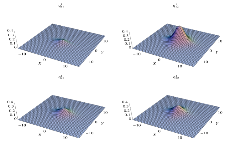
Figure 1: $(1,1)$-dromion plots with $p_{1}=\frac{1}{2}+\textrm{i}$, $q_{1}=\frac{1}{2}-\textrm{i}$ and $h_{12}=\frac{1}{2}$, $h_{13}=\frac{1}{4}$, $h_{14}=\frac{3}{4}$, $h_{23}=\frac{1}{3}$, $h_{24}=\frac{1}{2}$, $h_{34}=\frac{1}{3}$.

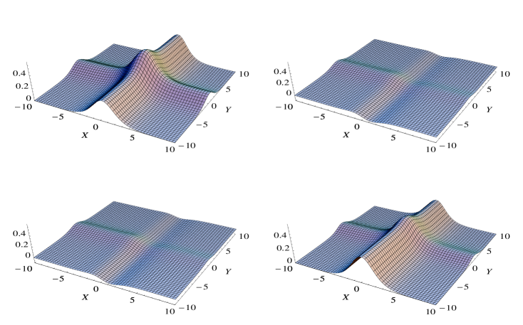
Figure 2: Plane waves corresponding to, clockwise from top left, $q_{11}^{1}$, $q_{12}^{1}$, $q_{22}^{1}$, $q_{21}^{1}$.

As can be seen from figure $1$, single dromions of differing heights occur in each of the fields $q_{11}$, $q_{12}$, $q_{21}$ and $q_{22}$. If we were to plot the $(1,1)$-dromion solution in the commutative (scalar) case (that is, if we were to choose $q$ and its complex conjugate to be of scalar rather than matrix form), we would obtain only one dromion in the single field $q$. This dromion and its plane waves would have the same basic structure as those above, and thus there would be no marked difference in the appearance of the dromions in the commutative and noncommutative cases. The main difference between the two situations concerns the number of parameters - a far greater number in the noncommutative case gives us more freedom to control the heights of the dromions, however some extra care has to be taken in choosing the parameters so that no singularities occur in the solution.

7.4 $(2,2)$-dromion solution - matrix case

In the scalar case [10], Gilson and Nimmo carried out a detailed asymptotic analysis of their $(M,N)$-dromion solution, and were able to obtain compact expressions for the phase-shifts and changes in amplitude that occur due to dromion interactions. They then used the results of this analysis to study a class of $(2,2)$-dromions with scattering-type interaction properties. The Hermitian matrix $H$ could be chosen in such a way so that some of the dromions had zero amplitude either as $t\rightarrow{-\infty}$ or as $t\rightarrow{+\infty}$.
 
 For the $(2,2)$-dromion solution in the matrix case, detailed calculations of this type are more complicated due to the large number of terms involved. However, we can adopt the same approach to carry out some of the more straightforward calculations. In particular, we obtain plots of the situation in which the $(1,1)^{\textrm{th}}$ dromion in each of the solutions $q_{11}^{2}$, $q_{12}^{2}$, $q_{21}^{2}$ and $q_{22}^{2}$ does not appear as $t\rightarrow{-\infty}$. These are depicted in figures $3$-$5$.
 
 To analyse this situation, we focus our attention on $q_{11}^{2}$ and consider $G_{11}^{2}$ in a frame moving with the $(1,1)^{\textrm{th}}$ dromion. We define

$$\hat{X} =X-2\Im({p_{1}})t,$$ (7.17a)

$$\hat{Y} =Y-2\Im({q_{1}})t,$$ (7.17b)

and consider the limits of $G_{11}^{2}$ as $t\rightarrow{-\infty}$. Let

$$\eta_{2} =\Re(p_{2})\left(X-2\Im(p_{2})t\right)$$

$$=\Re(p_{2})\left(\hat{X}-2(\Im(p_{2})-\Im(p_{1}))t\right),$$ (7.18a)

and similarly

$$\xi_{2} =\Re(q_{2})\left(Y-2\Im(q_{2})t\right)$$

$$=\Re(q_{2})\left(\hat{Y}-2(\Im(q_{2})-\Im(q_{1}))t\right).$$ (7.18b)

We choose to order the $p_{i},q_{i}$ ($i=1,2$) by means of their imaginary parts, so that $\Im(p_{1})>\Im(p_{2})$ and $\Im(q_{1})<\Im(q_{2})$. Thus, as $t\rightarrow{-\infty}$, $\eta_{2}\rightarrow{-\infty}$ and $\xi_{2}\rightarrow{+\infty}$. It can easily be shown that $\eta_{2}$, $-\xi_{2}$ determine the real parts of the exponents in $\alpha_{2}$, $\beta_{2}$ respectively, where $\alpha_{2}$, $\beta_{2}$ are defined as in (7.5), so that, as $t\rightarrow{-\infty}$, $\alpha_{2}$, $\beta_{2}\rightarrow{0}$ (and hence $\alpha_{2}^{*}$, $\beta_{2}^{*}\rightarrow{0}$ also). Therefore, by setting $\alpha_{2},\alpha_{2}^{*},\beta_{2},\beta_{2}^{*}\rightarrow{0}$ in $G_{11}^{2}$ and expanding the resulting determinant, we obtain a compact expression for $G_{11}^{2}$ as $t\rightarrow{-\infty}$, namely

$$G_{11}^{2}=-\alpha_{1}\beta_{1}^{*}\left(h_{2345678}^{1245678}-P_{1}h_{345678}^{145678}e^{2\eta}-Q_{1}h_{235678}^{125678}e^{-2\xi}+P_{1}Q_{1}h_{35678}^{15678}e^{2\eta-2\xi}\right).$$ (7.19)

Similar expressions can be obtained for the other three determinants $G_{12}^{2}$, $G_{21}^{2}$ and $G_{22}^{2}$ by considering an extension of (7.8) to the $(2,2)$-dromion case and interchanging columns appropriately: for example, we interchange columns $3$ and $4$, and $7$ and $8$, in the expansion of $G_{11}^{2}$ as $t\rightarrow{-\infty}$ to obtain an analogous expression for $G_{12}^{2}$. Thus we have, as $t\rightarrow{-}\infty$, compact expressions for the minors of $H$ governing the $(1,1)^{\textrm{th}}$ dromion in each of $G_{11}^{2}$, $G_{12}^{2}$, $G_{21}^{2}$, $G_{22}^{2}$, namely

$$\begin{pmatrix}G_{11}^{2}&G_{12}^{2}\\ G_{21}^{2}&G_{22}^{2}\\ \end{pmatrix}=-\alpha_{1}\beta_{1}^{*}\Biggl{\{}\begin{pmatrix}|h_{13}|&|h_{14}|\\ |h_{23}|&|h_{24}|\end{pmatrix}+P_{1}T\begin{pmatrix}{\begin{vmatrix}h_{12}&h_{13}\\ h_{22}&h_{23}\end{vmatrix}}&{\begin{vmatrix}h_{12}&h_{14}\\ h_{22}&h_{24}\end{vmatrix}}\\ {}&{}\\ {\begin{vmatrix}h_{11}&h_{13}\\ h_{21}&h_{23}\end{vmatrix}}&{\begin{vmatrix}h_{11}&h_{14}\\ h_{21}&h_{24}\end{vmatrix}}\end{pmatrix}e^{2\eta}\\ +Q_{1}T\begin{pmatrix}{\begin{vmatrix}h_{13}&h_{14}\\ h_{43}&h_{44}\end{vmatrix}}&{\begin{vmatrix}h_{13}&h_{14}\\ h_{33}&h_{34}\end{vmatrix}}\\ {}\\ {\begin{vmatrix}h_{23}&h_{24}\\ h_{43}&h_{44}\end{vmatrix}}&{\begin{vmatrix}h_{23}&h_{24}\\ h_{33}&h_{34}\end{vmatrix}}\end{pmatrix}e^{-2\xi}+P_{1}Q_{1}T\begin{pmatrix}{\begin{vmatrix}h_{12}&h_{13}&h_{14}\\ h_{22}&h_{23}&h_{24}\\ h_{42}&h_{43}&h_{44}\end{vmatrix}}&{\begin{vmatrix}h_{12}&h_{13}&h_{14}\\ h_{22}&h_{23}&h_{24}\\ h_{32}&h_{33}&h_{34}\end{vmatrix}}\\ {}\\ {\begin{vmatrix}h_{11}&h_{13}&h_{14}\\ h_{21}&h_{23}&h_{24}\\ h_{41}&h_{43}&h_{44}\end{vmatrix}}&{\begin{vmatrix}h_{11}&h_{13}&h_{14}\\ h_{21}&h_{23}&h_{24}\\ h_{31}&h_{33}&h_{34}\end{vmatrix}}\end{pmatrix}Te^{2\eta-2\xi}\Biggr{\}},$$ (7.20)

where $T=\text{diag}(-1,1)$. Since we have written out each minor matrix explicitly, rather than using the abbreviated notation as in (7.19) above, it can easily be seen that, by setting each of $h_{13},h_{14},h_{23},h_{24}$ equal to zero, the $(1,1)^{\textrm{th}}$ dromion in each of $q_{11}^{2},q_{12}^{2},q_{21}^{2}$ and $q_{22}^{2}$ will vanish as $t\rightarrow{-\infty}$. This is shown in figures $3$-$5$ below, where we have chosen $p_{1}=q_{2}=\frac{1}{2}+\textrm{i}$, $p_{2}=q_{1}=\frac{1}{2}-\textrm{i}$, and appropriate values of $h_{ij}$ ($i,j=1,\ldots,8$). (Note that in the plots of $q_{11}^{2}$ and $q_{12}^{2}$ in figure $3$, two of the dromions have very small amplitude). We have also shown, in figure $6$, a close-up of one of the dromion interactions at $t=0$.

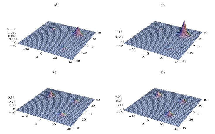
Figure 3: $(2,2)$-dromion plots at $t=-10$.

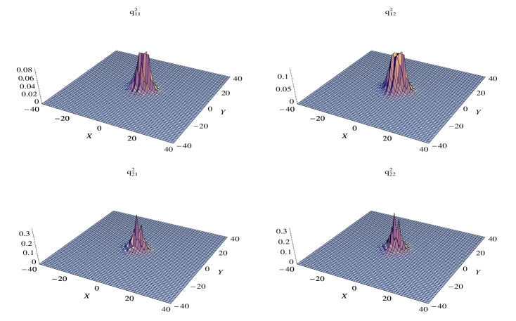
Figure 4: $(2,2)$-dromion plots at $t=0$.

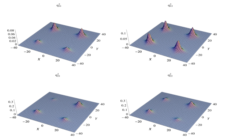
Figure 5: $(2,2)$-dromion plots at $t=10$.

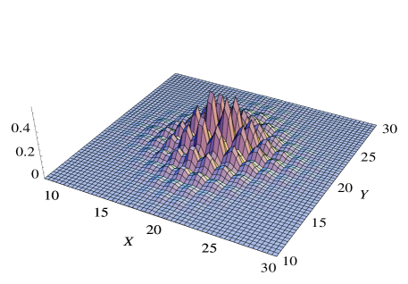
Figure 6: Detail of the $q_{22}^{2}$ dromion interaction shown in figure $4$.

8 Conclusions

In this paper we have derived a noncommutative version of the Davey-Stewartson equations and verified their quasiwronskian and quasigrammian solutions by direct substitution. The quasigrammian solution has then been used to obtain dromion solutions in the matrix case, which, if we were to consider these solutions in the scalar case, agree with the results of Gilson and Nimmo in [10]. We have obtained plots of the $(1,1)$-dromion solution and its plane waves, choosing the entries of the Hermitian matrix $H$ in such a way that our solution is always well-defined. In the $(2,2)$-dromion case, some of the more straightforward asymptotic calculations have been carried out, enabling us to obtain plots of the situation with one dromion vanishing as $t\rightarrow{-\infty}$.

Appendix

Here we prove the results of section 5. Consider a general quasideterminant of the form given by (5.1). Using the product rule for derivatives,

$$\Xi^{\prime}=D^{\prime}-C^{\prime}A^{-1}B+CA^{-1}A^{\prime}A^{-1}B-CA^{-1}B^{\prime}.$$ (A.1)

We modify slightly the approach of [11] and find that, if $A$ is a Grammian-like matrix with derivative

$$A^{\prime}=\sum_{i=1}^{k}E_{i}F_{i},$$ (A.2)

where $E_{i}$ $(F_{i})$ are column (row) vectors of comparable lengths, then

$$\Xi^{\prime} =D^{\prime}-CA^{-1}B+\sum_{i=1}^{k}(CA^{-1}E_{i})(F_{i}A^{-1}B)-CA^{-1}B^{\prime}$$

$$=\begin{vmatrix}A&B\\ C^{\prime}&\boxed{D^{\prime}}\end{vmatrix}+\begin{vmatrix}A&B^{\prime}\\ C&\boxed{0}\end{vmatrix}+\sum_{i=1}^{k}\begin{vmatrix}A&E_{i}\\ C&\boxed{0}\end{vmatrix}\begin{vmatrix}A&B\\ F_{i}&\boxed{0}\end{vmatrix}.$$ (A.3)

Note here that $`0$’ denotes the $2\times{2}$ matrix $\bigl{(}\begin{smallmatrix}0&0\\ 0&0\end{smallmatrix}\bigr{)}$. If, on the other hand, the matrix $A$ does not have a Grammian-like structure, we can once again write the derivative $\Xi^{\prime}$ as a product of quasideterminants as above by inserting the $2n\times{2n}$ identity matrix in the form

$$I=\sum_{k=0}^{n-1}(f_{k}\,e_{k})(f_{k}\,e_{k})^{T},$$ (A.4)

with $e_{k}$, $f_{k}$ defined as before, so that $(f_{k}\,e_{k})$ denotes the $2n\times{2}$ matrix with the $(2n-2k)^{\textrm{th}}$ and $(2n-2k-1)^{\textrm{th}}$ entries equal to 1 and every other entry 0. Then we find that

$$\Xi^{\prime}=\begin{vmatrix}A&B\\ C^{\prime}&\boxed{D^{\prime}}\end{vmatrix}+\sum_{k=0}^{n-1}\begin{vmatrix}A&\begin{array}[]{cc}f_{k}&e_{k}\end{array}\\ C&\boxed{\begin{array}[]{cc}0&0\\ 0&0\end{array}}\end{vmatrix}.\begin{vmatrix}A&B\\ \begin{array}[]{c}(A^{2n-2k-1})^{\prime}\\ (A^{2n-2k})^{\prime}\end{array}&\boxed{\begin{array}[]{c}(B^{2n-2k-1})^{\prime}\\ (B^{2n-2k})^{\prime}\end{array}}\end{vmatrix},$$ (A.5)

where $A^{k}$ denotes the $k^{\textrm{th}}$ row of $A$. It is also possible to obtain a column version of the derivative formula by inserting the identity in a different position. We now use the formulae (A.3) and (A.5) to derive expressions for the derivatives of the quasideterminants $Q(i,j)$, $R(i,j)$.
 
 Consider the quasiwronskian $Q(i,j)$ defined in section 4.2, namely

$$Q(i,j)=\begin{vmatrix}\widehat{\Theta}&\begin{array}[]{cc}f_{j}&e_{j}\end{array}\\ \Theta^{(n+i)}&\boxed{\begin{array}[]{cc}0&0\\ 0&0\end{array}}\end{vmatrix}.$$ (A.6)

Calculation of the derivatives of $Q(i,j)$ requires knowledge of the following result [11], that for arbitrarily large $n$,

$$Q(i,j)=\begin{cases}-I_{2}&i+j+1=0,\\ \bigl{(}\begin{smallmatrix}0&0\\ 0&0\end{smallmatrix}\bigr{)}&\text{$i<0$ or $j<0$ and $i+j+1\neq{0}$}.\end{cases}$$ (A.7)

We utilise the dispersion relations for the ncDS system (2.5a-d), found by considering the Lax pairs (2.1a,b) in the trivial vacuum case, giving, for $\theta$ an eigenfunction of $L$, $M$,

$$\theta_{x} =-\sigma{J}\theta_{y},$$ (A.8a)

$$\theta_{t} =\textrm{i}J\theta_{yy},$$ (A.8b)

and since $\Theta=\left(\theta_{1},\ldots,\theta_{n}\right),$ it follows that

$$\Theta_{x} =-\sigma{J}\Theta_{y},$$ (A.9a)

$$\Theta_{t} =\textrm{i}J\Theta_{yy}.$$ (A.9b)

Thus, using (A.5), we have

$${Q}(i,j)_{y} =Q(i+1,j)+\sum_{k=0}^{n-1}Q(i,k)Q(-k,j),$$ (A.10a)

$${Q}(i,j)_{x} =-\sigma\left({J}Q(i+1,j)+\sum_{k=0}^{n-1}Q(i,k)JQ(-k,j)\right),$$ (A.10b)

$${Q}(i,j)_{t} =\textrm{i}\left(JQ(i+2,j)+\sum_{k=0}^{n-1}Q(i,k)JQ(-k,j)\right).$$ (A.10c)

These can be simplified using (A.7), leaving the derivatives as given in (5.5).
 
 We can apply a similar procedure to determine the derivatives of the quasigrammian $R(i,j)$ defined in section 4.4. The dispersion relations are found by considering the adjoint Lax pairs (4.14a,b) in the trivial vacuum case, giving, for $\rho$ an eigenfunction of $L^{{\dagger}}$, $M^{{\dagger}}$,

$$\rho_{x} =-\frac{1}{\sigma}{J}\rho_{y},$$ (A.11a)

$$\rho_{t} =\textrm{i}J\rho_{yy},$$ (A.11b)

and since $P=(\rho_{1},\ldots,\rho_{n})$, we have

$$P_{x} =-\frac{1}{\sigma}{J}P_{y},$$ (A.12a)

$$P_{t} =\textrm{i}JP_{yy}.$$ (A.12b)

We also recall that from our construction of the binary Darboux transformation in section 4.3, the potential $\Omega(\phi,\psi)$ satisfies the relations (4.15a-c), from which it follows that

$$\Omega(\Theta,P)_{y} =P^{{\dagger}}\Theta,$$ (A.13a)

$$\Omega(\Theta,P)_{x} =-\sigma{P}^{{\dagger}}J\Theta,$$ (A.13b)

$$\Omega(\Theta,P)_{t} =\textrm{i}\left(P^{{\dagger}}J\Theta^{(1)}-P^{{\dagger}(1)}J\Theta\right),$$ (A.13c)

where ^(k) denotes the $k^{\textrm{th}}$ $y$-derivative. Thus, using (A.3), we calculate the derivatives of $R(i,j)$ and find that they are identical to those of $Q(i,j)$ in (5.5).

References

- [1] M. J. Ablowitz and P. A. Clarkson. Solitons, nonlinear evolution equations and inverse scattering. Cambridge University Press, 1991.
- [2] M. J. Ablowitz and C. L. Schultz. Action-angle variables and trace formula for D-bar limit case of Davey-Stewartson I. Physics Letters A, 135(8,9): 433–437, 1989.
- [3] M. Boiti, J. J.-P. Leon, L. Martina, and F. Pempinelli. Scattering of localized solitons in the plane. Physics Letters A, 132, 1988.
- [4] A. Davey and K. Stewartson. On three-dimensional packets of surface waves. Proceedings of the Royal Society of London A, 338: 101–110, 1974.
- [5] A. Dimakis and F. Müller-Hoissen. Multicomponent Burgers and KP hierarchies, and solutions from a matrix linear system. Symmetry, Integrability and Geometry: Methods and Applications, 5(2): 1–18, 2009.
- [6] A. S. Fokas and P. M. Santini. Coherent structures in multidimensions. Physical Review Letters, 63(13): 1329–1334, 1989.
- [7] N. C. Freeman and J. J. C. Nimmo. Soliton solutions of the Korteweg–de Vries and Kadomtsev–Petviashvili equations: the Wronskian technique. Physics Letters, 95A(1): 1–3, 1983.
- [8] I. Gelfand, S. Gelfand, V. Retakh, and R. L. Wilson. Quasideterminants. Advances in Mathematics, 193: 56–141, 2005.
- [9] I. Gelfand and V Retakh. Determinants of matrices over noncommutative rings. Functional Analysis and its Applications, 25(2): 91–102, 1991.
- [10] C. R. Gilson and J. J. C. Nimmo. A direct method for dromion solutions of the Davey-Stewartson equations and their asymptotic properties. Proceedings of the Royal Society of London A, 435: 339–357, 1991.
- [11] C. R. Gilson and J. J. C. Nimmo. On a direct approach to quasideterminant solutions of a noncommutative KP equation. Journal of Physics A: Mathematical and Theoretical, 40: 3839–3850, 2007.
- [12] M. Hamanaka. On reductions of noncommutative anti-self-dual Yang-Mills equations. Physics Letters B, 625: 324–332, 2005.
- [13] J. Hietarinta and R. Hirota. Multidromion solutions to the Davey-Stewartson equation. Physics Letters A, 145(5): 237–244, 1990.
- [14] R. Hirota. The Direct Method in Soliton Theory. Cambridge University Press, 2004.
- [15] O. Lechtenfeld, L. Mazzanti, S. Penati, A. D. Popov, and L. Tamassia. Integrable noncommutative sine-Gordon model. Nuclear Physics B, 705(3): 477–503, 2005.
- [16] O. Lechtenfeld and A. D. Popov. Journal of High Energy Physics, JHEP0111, 2001.
- [17] C. Li. Private communication.
- [18] V. B. Matveev and M. A. Salle. Darboux transformations and solitons. Springer-Verlag, 1991.
- [19] J. E. Moyal. Quantum mechanics as a statistical theory. Proceedings of the Cambridge Philosophical Society, 45: 99–124, 1949.
- [20] M. C. Ratter. Grammians in nonlinear evolution equations. PhD thesis, University of Glasgow, 1998.
- [21] C. L. Schultz, M. J. Ablowitz, and D. Bar Yaacov. Davey-Stewartson I system: a quantum (2+1)-dimensional integrable system. Physical Review Letters, 59(25): 2825–2828, 1987.