A Minimum Variance Method for
Problems in Radio Antenna Placement

Abstract

Aperture synthesis radio telescopes generate images of celestial bodies from data obtained from several radio antennas. Placement of these antennas has always been a source of interesting problems. Often, several potentially contradictory objectives like good image quality and low infra-structural cost have to be satisfied simultaneously.

In this paper, we propose a general Minimum Variance Method that focuses on obtaining good images in the presence of limiting situations. We show its versatility and goodness in three different situations: (a) Placing the antennas on the ground to get a target Gaussian UV distribution (b) Staggering the construction of a telescope in the event of staggered budgets and (c) Whenever available, using the mobility of antennas to obtain a high degree of fault tolerance.

1 Introduction

The technique of interferometric aperture synthesis has brought about a revolution in the field of radio astronomy in the past four decades[12]. The technique works by synthesizing images from signals obtained from antennas spread over a large distance. For a quick introduction to basic interferometric radio astronomy, please see the Appendix A.

Most radio telescopes today use the concept of interferometric aperture synthesis. The Very Large Array (VLA) in the USA with 27 antennas and the Giant Meter wave Radio Telescope (GMRT) in India with 30 antennas are good examples of such telescopes. A multi-purpose new generation radio telescope called the Square Kilometer Array (SKA) has been proposed (see Section 2 and the website http://www.skatelescope.org), and is currently in the design phase.

An important problem in the field of interferometric radio-astronomy is to find the antenna placement on the ground that generates a required UV-distribution. This problem is a computationally difficult one [10]. In addition to antenna placement on purely scientific merit, other dimensions are added when we consider logistical and financial issues. For example, given a particular placement, what is the optimum cable layout? What trade-off can be struck between scientific merit and wire length and other infrastructure costs?

In this paper we look at three important problems that arise chiefly from the standpoint of astronomic merit:

• The first is a general problem. It turns out that a Gaussian distribution of UV points in the radial direction and a uniform distribution in the azimuthal direction is desirable for Gaussian beams [2]. It has been observed empirically that a uniform random placement of antennas on the XY plane yields a radially tapering UV distribution [15]. A simple calculation shows that this is as expected. However, it may not be sufficiently close, particularly when some antenna positions are not feasible (say, because of geopolitical constraints). How does one rectify this?

• The second is motivated primarily by financial considerations. Suppose the funding for the project is spread over a period of time as is likely to be in the case of the SKA. It is also reasonable to assume that the construction of the entire array will take time, because of logistical reasons. In such a scenario, one would still like to perform experiments and get good quality images in the meantime. Can we come up with a placement schedule that enables such a graceful upgrading?

  This question has been raised in the past in this context [10] and others [14]. A more recent version of this question concerns expanding existing arrays [8]. Their solution involves evaluating every antenna configuration. This is expensive in the scenario where the number of antennas is large, and there is limited time for rearrangement of antennas between successive experiments.

• The third concerns mobile antennas. While there are a limited number $M$ of antennas available, there are several more pads that can host an antenna each. Ideally, an experiment would require antennas on at least some of those pads. Consider the case when only some $N$ of those antennas are available (due to maintenance reasons or involvement with other experiments, the rest are unavailable). On which $N$ pads out of the required pads should we place the antennas?

We propose a Minimum Variance Method (MVM) that tackles the above problems. It is interesting to note that the same framework is useful for these seemingly different problems.

Informally, this technique involves choosing $N$ out of $M$ (where $M\geq N$) possible locations for placing the antennas. To achieve this, we start by placing an antenna on each of the M locations. Then, we iteratively remove $M-N$ antennas, one at a time, such that we stay “close” to the target UV distribution. Our solution takes $O((M-N)\cdot M^{3})$ time, which is an improvement over brute force solutions. A brute force solution would involve comparing distributions that result from all $\binom{M}{M-N}$ choices for antenna removal.

We conduct our experiments on a random placement scheme, on the placement data of 120 antennas/stations of the proposed Australian SKA (see next section), and on the placement data of the 24 antennas of the Sub-millimeter Array at Mauna Kea, Hawaii (see Section 4).

Some relevant literature is discussed in the next section. In Section 3, we present the Minimum Variance Method. Section 4 shows how the technique applies to the three problems stated above, along with the experimental results. Section 5 concludes the paper.

2 Previous Work

This work has been done keeping in mind the proposed Square Kilometre Array (SKA) project. The SKA is an ambitious multi-purpose new generation radio telescope with a total collecting area of approximately one square kilometer, designed to work over a wide range of radio frequencies – $70~{}\rm MHz$ to $25~{}\rm GHz$. The telescope is expected to play a major role in answering key questions in modern astrophysics and cosmology. This high resolution array will be $50$ times more sensitive, and will be able to cover the sky $10000$ times faster than any imaging radio telescope array previously built. It is hoped that besides exploratory astronomy, the SKA will provide insights into many interesting questions about the birth and evolution of galaxies, origins of magnetism, possibility of existence of life on some other planet, verification of general relativity etc. For more details see [4].

A lot of work has been done in the past on the problem of antenna placement. They range from constructing the array ab-initio to incrementing an existing one. We cite a few important example papers here; the reader is encouraged to read the citations therein.

In 1989, Treloar compared various array configurations in terms of the amount of sampling of different regions in the UV-plane and the absence of holes therein, for fixed declinations [15]. Among the configurations studied was the spiral, with higher concentration towards the centre with distribution of antennas varying with the radius. Cohanim et al posed the array design problem as a multi-objective optimization problem of maximizing image performance and minimizing cable-length using genetic algorithms and simulated annealing [10]. Motivated by the work of Takeuchi et al [14], they mention the problem of phased deployment of the antennas.

Lonsdale and Cappallo make the case for a large number of antennas, of the order of a thousand [9]. Among other factors including high fidelity and good UV-coverage, they argue that a large number of stations (a collection of antenna imaging a specific region of the sky) relieves the dependence on the earth’s rotation for a comprehensive sampling of the UV-plane. They also present log-spiral and hybrid (log-spiral for inner regions and pseudo-random star for the outer regions) antenna layouts, which have the advantages of good UV-coverage towards the centre, a wide range of baseline lengths and shorter communication cables in general. Problems of insufficient coverage and long cable lengths appear in the outer regions. Several variants of a technique that seeks to maximize the distance between UV points have also been explored in the past ([1] and [6]).

Karastergiou et al [8] adapted the approach of Boone [1] and Cornwell [6] to the case when there are more potential sites (called pads) than antennas, and one has to choose a configuration for an experiment by shifting the antennas among the pads. The work stemmed from an observation of Boone [2] that if the density of the UV-plane is sparse, it is advisable to spread the Gaussian along a radial direction a bit so that all regions of the UV-plane have at least a sample point. The technique they used was inspired by the physical phenomenon of charges spreading on a closed 2-D surface in order to minimize the energy. Their idea is to affect all the discrete shifts and see which configuration results in the least energy, thus satisfying the experimental requirements.

Su et al [13] proposed the uniform weight approach. The problem that they tackle is of choosing sites for placement of antennas given several more candidate sites. They aim for a uniform and complete UV-distribution in the absence of a-priori information on the objectives of the experiments. Their method involves assigning a weight to a UV point that is equal to its distance from the nearest UV point. An antenna is thus assigned the sum of all distances of the relevant UV points. The antenna that has the least weight is dropped.

Finally, we mention the tomographic projection method of de Villiers [7] in which he compares the projection of an imperfect and an ideal UV distributions onto one dimension. The discrepancy yields correction terms that are mapped to new antenna positions. Doing this in several directions allows one to get close to the ideal configuration.

3 The Minimum Variance Method

The basic idea of this paper is as follows. First, we divide the UV-plane into $p$ regions. Division is necessary because we wish a distributed removal of points so that some portion of the UV plane is not denuded of UV points. The general way to capture the notion of distribution is to grid the plane and then talk of “points per grid unit” [1, 13]. How this division is done will be described towards the end of this section. We note, however, that the MVM can accommodate any scheme for division of the UV plane in principle. The desired UV distribution dictates the number of UV points each region should hold.

Our algorithm starts with $M>N$ antennas and removes $M-N$ antennas, one at a time, in an iterative fashion. Suppose that at the start of the $r^{\tiny\hbox{th}}$ iteration, there are $p^{[r]}$ regions and $M^{[r]}$ antennas. Then, $M^{[r]}-1$ UV points will be dropped as a result of the removal of one antenna during the $r^{\tiny\hbox{th}}$ iteration.

Depending on the requirements of the UV distribution, we would like the removal of $R_{i}^{[r]}$ UV points from the $i^{\tiny\hbox{th}}$ region in the $r^{\tiny\hbox{th}}$ iteration. However, in general, the number of UV points dropped from the region $i$ due to removal of antenna $j$ would be different, say $w_{i}(j)$.

We capture the discrepancy between the actual and ideal UV points dropped in every region by removing the antenna $j$ with the following term:

$$Var(j)=\sum_{i=1}^{p^{[r]}}(w_{i}(j)-R_{i}^{[r]})^{2}.$$

We now drop the antenna that has the least $Var(.)$ value. In short, the logic for deletion of the $N$ antennas is this:

1. while there are more than $N$ antennas remaining do

2. for each remaining antenna $j$

3. Calculate $Var(j)$.

4. end for

5. Remove the antenna that has the least $Var(.)$.

6. end while

This antenna removal routine can be tweaked for different problems. Let us now estimate the worst case time complexity of this routine. There are at most $M-N$ antennas to be removed. Every remaining antenna is a candidate for removal, of which there are at most $M$. For every such candidate we go through the (at most $M^{2}$) UV points, identify those associated with the candidate, and determine which region they belong to, in order to calculate $Var(j)$. Thus, we need at most $O((M-N)M(M^{2}+p))=O((M-N)\cdot M^{3})$ steps.

But for a rotation for changing coordinates, a UV point is defined as $u=\frac{X_{1}-X_{2}}{\lambda}$ and $v=\frac{Y_{1}-Y_{2}}{\lambda}$ for every pair $(X_{1},Y_{1})$ and $(X_{2},Y_{2})$ of XY coordinates (see Appendix A). Therefore it is sufficient to work with the distribution that the XY coordinate differences may follow. In all our experiments, without loss of generality, we take $\lambda=1$.

There are at least two natural choices for the shape of the regions into which the UV plane can be divided. One is into concentric circles due to radial symmetry. The other is into coaxial ellipses because of the facts that the UV tracks are elliptical in general, and that in several earth rotation aperture synthesis telescopes, a prolonged coverage is desirable. In a scheme that removes antennas progressively from a large set, there are two options regarding the number of regions. The first is to adaptively reduce the number of regions in accordance with the reduced antennas. In doing so, the configuration in an iteration will mimic that in the previous iteration. The second option is to stick to the same number of regions throughout, so that all intermediate configurations will mimic the final. We demonstrate the use of different UV plane division schemes, both in terms and shape and number of regions, in our experiments.

4 Applications

4.1 Problem 1: UV to XY

The UV distribution that is desired in most cases is a Gaussian along the radial and uniform along the azimuthal direction. As the next lemma indicates, a random distribution of antennas on the ground, that is, the XY-plane, gives a tapering distribution in the UV-plane.

Lemma: Consider a $S\times S$ square grid having $(S+1)^{2}$ lattice points in the XY plane. Suppose that we choose each lattice point independently with probability $0\leq p\leq 1$ and look at the UV distribution generated by the chosen points. Then the expected number of UV points at the position $(x,y)$, where $-S\leq x,y\leq S$, is $p^{2}(S+1-|x|)(S+1-|y|)$.

Proof: For the given $S\times S$ square grid, the number of pairs of lattice points $(X_{1},Y_{1})$ and $(X_{2},Y_{2})$ such that $X_{2}-X_{1}=x$ and $Y_{2}-Y_{1}=y$ is $(S+1-|x|)(S+1-|y|)$. Since each such contributing pair is expected to be chosen with probability $p^{2}$, linearity of expectation gives the desired result. $\square$

The above lemma indicates that a random XY distribution induces more UV points corresponding to short XY distance pairs. This tapers off for longer distances. With this as a starting point, we apply the Minimum Variance Method to arrive at the target Gaussian.

Given: (i) A geography, that is, dimensions of the land on which to place antennas. (ii) The number of antennas that are to be installed and (iii) The amplitude $a_{f}$ of the desired Gaussian UV plane.

Goal: To find a placement of $N$ antennas that yields a Gaussian UV distribution centered at the origin having an amplitude $a_{f}$ and standard deviation $\sigma=B/4$, where $B$ is the largest inter UV point distance.

Approach: We start with an overkill of antennas. Instead of the required $N$, we start with $M\approx 2N$ antennas and place them randomly on the XY-plane. Our random choice results in a distribution of points on the UV-plane that deviates from the desired Gaussian. We now try to minimize the deviation from the target Gaussian by iteratively removing an antenna that causes the minimum deviation from the desired Gaussian. We stop when we have removed $M-N$ antennas.

Figure 1 illustrates conceptually the line of approach. The two meshes indicate the starting and the final distributions. The effort will be towards minimizing the discrepancy between the distributions at every iteration when we remove an antenna.

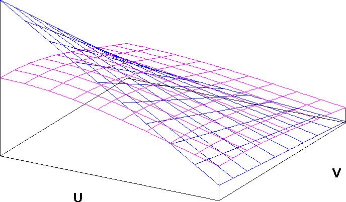
Figure 1: The steeper curve is generated by an initial random distribution of the $M$ antennas while the pink curve is the desired Gaussian.

Details: As stated earlier, our random choice results in a distribution of points on the UV-plane that deviates from the desired Gaussian.

We then draw a fixed number $p=B/d$ of concentric circles with the radii increasing in arithmetic progression of common difference $d$. We will show how to fix $d$ shortly. Given these annuli, it is possible to plot a density histogram of the number $q_{i}^{[\tiny\hbox{init}]}$ of UV-points that lie in the annuli bounded by the circles $i$ and $i+1$ (for $1<i<p$; $q_{1}^{[\tiny\hbox{init}]}$ being the number of points in the central circle) versus distance. Thus, the total number of UV points initially is $Q^{[\tiny\hbox{init}]}=\sum_{i=1}^{p}q_{i}^{[\tiny\hbox{init}]}=M\cdot(M-1)/2$ and area under this histogram is $A^{[\tiny\hbox{init}]}=d\cdot\sum_{i=1}^{p}q_{i}^{[\tiny\hbox{init}]}=d\cdot M\cdot(M-1)/2$.

Let us now fix $d$. The area under half the Gaussian centered at the origin with amplitude $a$ and having a standard deviation of $\sigma$ is given by $a\sigma\sqrt{\frac{\pi}{2}}$ (see Appendix B). Thus, given $a_{f}$, $\sigma$ and the final number $N$ of antennas, we have $a_{f}\sigma\sqrt{\frac{\pi}{2}}=\frac{d\cdot N\cdot(N-1)}{2}$. Therefore, $d=\frac{a_{f}\sigma\sqrt{\frac{\pi}{2}}}{\frac{N\cdot(N-1)}{2}}=\frac{a_{f}B\sqrt{\frac{\pi}{2}}}{2N\cdot(N-1)}$.

As has been mentioned previously, the central idea behind the present approach is to crop the initial curve to fit the Gaussian. Let the number of antennas remaining at the end of the $r^{th}$ iteration ($1\leq r\leq M-N$) be $M^{[r]}=M-r$. Then, $M^{[0]}=M$. Note that removal of an antenna during the $r^{th}$ iteration results in the removal of $M^{[r-1]}-1$ UV-points, which in turn results in a reduction of the area under the curve from $A^{[r-1]}$ to $A^{[r]}=d\cdot M^{[r]}\cdot(M^{[r]}-1)/2$.

We try to minimize the deviation from Gaussian by iteratively removing the antenna that causes the maximum deviation from the desired Gaussian. We use $A^{[r]}=d\cdot M^{[r]}\cdot(M^{[r]}-1)/2=a\sigma\sqrt{\frac{\pi}{2}}$, to get $a=\frac{d\cdot(M-r)\cdot(M-r-1)/2}{\sigma\sqrt{\frac{\pi}{2}}}.$

With $a$ determined (and $\sigma$ already being fixed), the expected Gaussian is uniquely defined. The vertical coordinate in the Gaussian distribution at $x=i$ is given by the formula $ae^{-\frac{d\cdot(i-1/2)^{2}}{2\sigma^{2}}}$. If $q_{i}^{[r-1]}$ is the number of UV points remaining in region $i$ at the end of iteration $r-1$, then the number of UV points we would like to remove from $i^{\tiny\hbox{th}}$ region in $r^{\tiny\hbox{th}}$ iteration is

$$R_{i}^{[r]} = q_{i}^{[r-1]}-\frac{d\cdot(M-r)\cdot(M-r-1)/2}{\sigma\sqrt{\frac{\pi}{2}}}\cdot e^{-\frac{d\cdot(i-1/2)^{2}}{2\sigma^{2}}}.$$

For each region $i$, let $w_{i}(j)$ be the number of UV-points that would be deleted from the region $i$ if the antenna $j$ is removed. Then, as per the Minimum Variance Method, we choose that antenna $j$ for removal which has got the least value of

$$Var(j)=\sum_{i=1}^{p}(w_{i}(j)-(q_{i}^{[r-1]}-\frac{d\cdot(M-r)\cdot(M-r-1)/2}{\sigma\sqrt{\frac{\pi}{2}}}\cdot e^{-\frac{d\cdot(i-1/2)^{2}}{2\sigma^{2}}}))^{2}.$$

For the experiment, we set a goal of generating a Gaussian distribution on the UV plane using $N=28$ antennas with $a_{f}=70$. We start with an initial set of $M=48$ antennas that are generated randomly as shown in Figure 2(a). The geography that we use, and the randomly generated antenna positions yields $B\approx 11180$ wavelengths. Then, $d\approx 6470$ wavelengths.

Figure 2(c) shows the UV-distribution generated by these antennas. The Density Histogram of the distribution is shown in Figure 2(e). Notice that the histogram deviates from the desired Gaussian at several places.

Figure 2(f) is the cropped histogram arrived at finally. Observe that this histogram is closer to Gaussian than the initial one. Figures 2(d) and 2(b) show the final UV and XY distributions respectively.

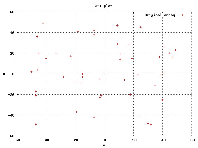
(a) The initial set of antennas

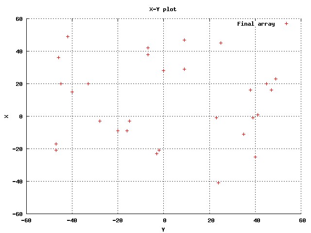
(b) The final set of antennas

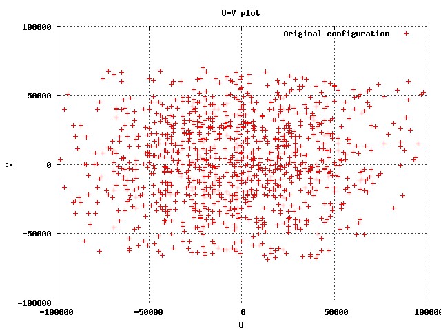
(c) The initial UV-distribution

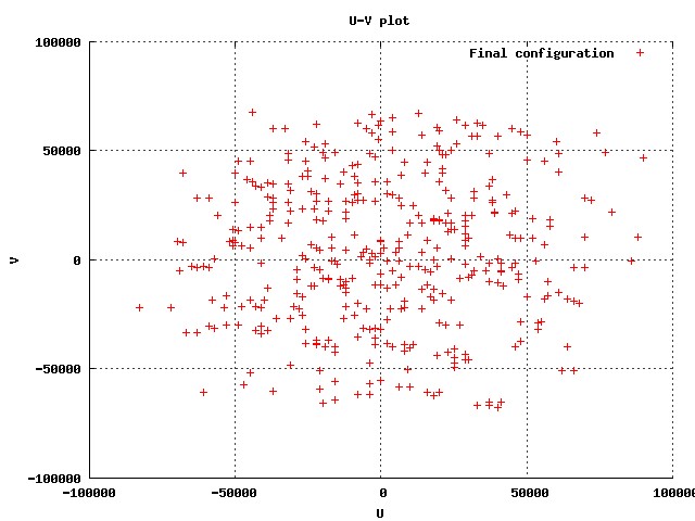
(d) The final UV-distribution

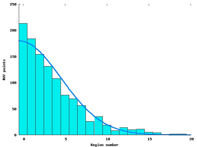
(e) The initial UV-density histogram

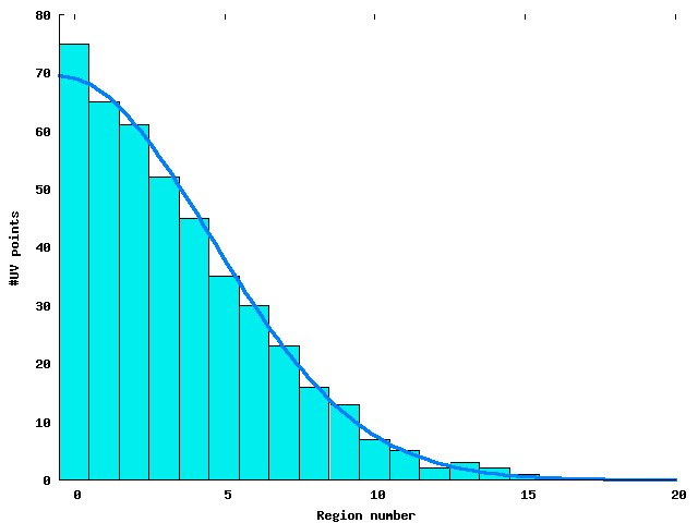
(f) The final UV-density histogram

Figure 2: UV to XY

4.2 Problem 2: Staggered Construction

Statement: A telescope of $M$ antennas has been proposed with all the sites identified. However, the telescope construction has to be staggered and it has to be built in phases since the funding becomes available in small chunks over a time period. Suppose that we are given a budget of $N$ antennas for Phase 1. Which $N$ of the total $M$ antennas should we construct in Phase 1?

Ideally one would like to start making quality observations after completion of Phase 1 itself which means that the UV-distribution that is generated by Phase 1 antennas should be a good approximation of the final UV-distribution that we would get after placing all $N$ antennas.

If $M$ is even, then we choose $p^{[0]}=M-1$ ellipses with $M/2$ UV-points per ellipse. Else, we choose $p^{[0]}=M$ ellipses with $(M-1)/2$ UV-points per ellipse. One ellipse is chosen for every $M$ of all the elliptical UV-tracks sorted by their $u^{2}+\frac{v^{2}}{\sin^{2}\delta}$. We aim for the removal of the same number of UV points from each region during every iteration. Thus, $R_{i}^{[r]}=\frac{M^{[r]}-1}{p^{[r]}}$, and

$$Var(j)=\sum_{i=1}^{p^{[r]}}(w_{i}(j)-\frac{M^{[r]}-1}{p^{[r]}})^{2}.$$

4.2.1 Experimental Results

We ran the experiment on the scaled down version of the Australian SKA for $M=120$ antenna locations. Figures 3(a) and 3(b) show the XY plane when populated with all the $120$ antennas and after removal of $40$ antennas and $80$ antennas respectively.

Since the $Z$ coordinates of the antennas also contribute to defining the UV plane, we provide the corresponding XZ plots along with the XY plots. Figures 3(c) and 3(d) show the corresponding XZ planes.

Figures 3(e) and 3(f) show the corresponding UV-planes. The hour angle used is $0^{\circ}$ and the declination $-30^{\circ}$.

Note that by our scheme, more antennas are removed towards the center of the log-spiral. Thus, it is more effective when $N$ is large. Also observe that by making use of the same Minimum Variance Method, we can create a construction plan for all remainder phases of the telescope building which has a steadily improving UV-coverage.

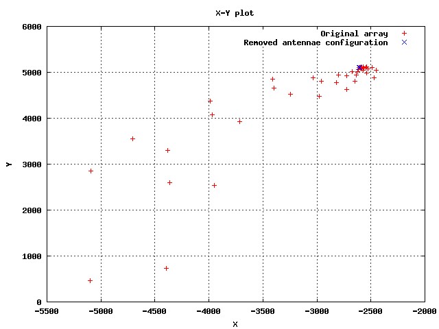
(a) XY plane–initial and 40 removed antennas

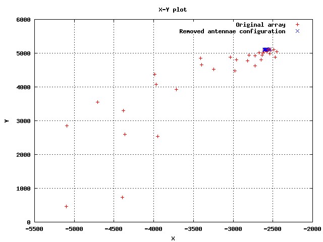
(b) XY plane–initial and 80 removed antennas

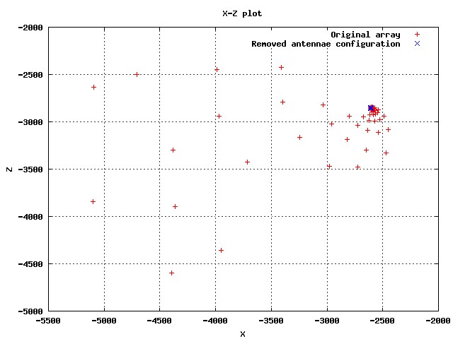
(c) XZ plane–initial and 40 removed antennas

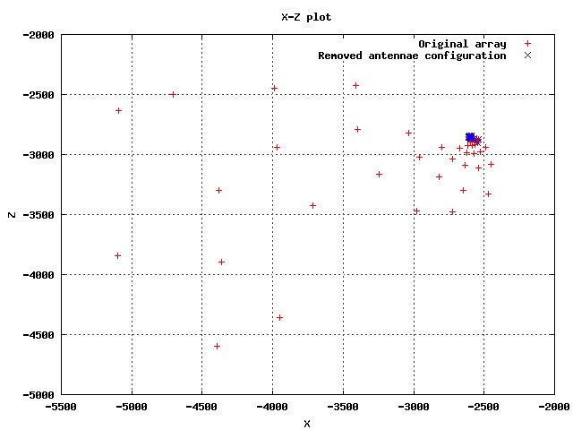
(d) XZ plane–initial and 80 removed antennas

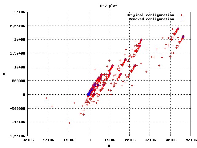
(e) The UV plane–initial and 40 removed antennas

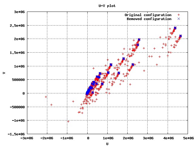
(f) The UV plane–initial and 80 removed antennas

Figure 3: Results for the proposed Australian SKA configuration.

4.3 Problem 3: Mobile Antennas

Statement: Suppose there are $L$ pads (for mounting $L$ antennas), but only $M\leq L$ mobile antennas pre-placed on $M$ pads. Suppose that an astronomer requests these $M$ antennas for some observation. However, only $N$ out of these $M$ can be allocated (say, because of maintenance reasons, or some being needed for another experiment). Our problem is to choose $N$ out of the $M$ antenna pads that best approximate the desired UV pattern generated by fully functional pre-placed $M$ antennas. Having done that, the antennas can be shifted to the recommended $N$ pads.

The parameters set for the previous problem in Subsection 4.2 carries through exactly. We did the experiment on Sub Millimeter Array data [8]. We assume the failure of $5$ of the $24$ antennas. Thus, in this setting, $M=24$ and $N=19$. Figure 4(a) shows the initial and final XY planes and 4(b) shows the XZ plane. Figure 4(c) show the resultant UV distributions. Using the output of the algorithm, one can recommend which $19$ pads can be used.

(a) The XY plane

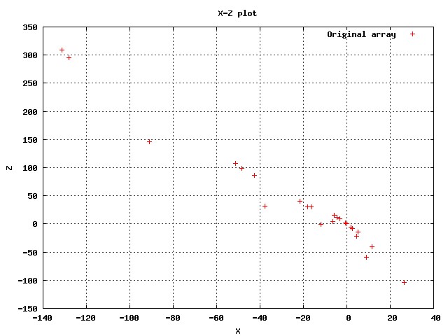
(b) The XZ plane

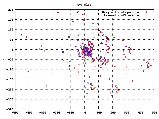
(c) The UV plane

Figure 4: Results for SMA configuration (mobile antennas)

5 Conclusions and Future Work

In this paper we proposed and studied a Minimum Variance Method that can be used in many radio antenna placement scenarios. We applied the method in three different situations effectively (i) obtaining ab-initio smooth Gaussian UV distributions (ii) incremental construction of very large aperture synthesis arrays and (iii) achieving fault tolerance in mobile antennas. We also report experiments that indicate the usefulness of this method. In addition versatility, this method is quite efficient when compared to the brute force method or minor improvements thereof.

In this paper, the only criterion that we considered for placing the antennas is image quality. It remains to come up with solutions that take into account logistical factors like wire length minimization, roadway utilization and so on.

Appendix A Aperture Synthesis Primer

It is a well-known fact in astronomy that the angular resolution of a telescope is proportional to $\lambda/D$ where $\lambda$ is the wavelength of the waves to be observed, and $D$ is the diameter of the telescope aperture. In order to observe celestial bodies in the long wavelength ranges ($1\text{mm}$ to $10\text{m}$), we need antennas with diameters of the order of hundreds of kilometers. Obviously, such antennas are practically impossible to build, manoeuver and maintain. Fortunately, it has been shown that several antennas can be used instead of a single big one. Several radio telescopes have been constructed in the past based on this principle of aperture synthesis. These telescopes have helped astronomers in discovering various celestial bodies like quasars, pulsars etc.

In this Appendix we quickly recap some concepts and terminology pertinent to this paper. The interested reader is referred to [3] and [5] for an excellent treatment of the subject.

Let us first consider the case of two antennas. Consider a rectilinear coordinate system $(u,v,w)$ such that the $w$-axis points in the direction that is to be the center of the synthesized field of view. Let $\mathbf{s_{0}}$ be the unit vector along the w-axis.

Assigning a direction and treating the shortest distance between the two antennas as the magnitude, we can speak of a baseline vector. Let the baseline vector be $\mathbf{b}=u\hat{u}+v\hat{v}+w\hat{w}$. Let $l$, $m$ and $n$ be the direction cosines of an element in the celestial sphere. Let $\mathbf{s}=l\hat{u}+m\hat{v}+n\hat{w}$ be a position vector of another element close by. Then, $\mathbf{b.s}=ul+vm+wn$ and $\mathbf{b.s_{0}}=w$.

Let $A(l,m)$ be the response of the antennas corresponding to a baseline in the direction specified by $(l,m)$. Further, let $A_{0}$ be the response of the antennas at the beam center. Then, $\mathcal{A}(l,m)=\frac{A(l,m)}{A_{0}}$ is called the normalized antenna reception pattern. The spatial correlation function of the electric field at the antennas corresponding to the baseline $\mathbf{b}$ is defined as

$$V(u,v,w)=\int_{-\infty}^{\infty}\int_{-\infty}^{\infty}\mathcal{A}(l,m)I(l,m)e^{-2\pi i[ul+vm+w(\sqrt{1-l^{2}-m^{2}}-1)]}\frac{dldm}{\sqrt{1-l^{2}-m^{2}}}$$

where $I(l,m)$ is the radio brightness in the $(l,m)$ direction, assuming that both the antennas are identically polarized.

Obtaining $I(l,m)$, our aim, is simplified to evaluating the inverse of a 2-D Fourier transform if $w=0$ :

$$V(u,v)=\int_{-\infty}^{\infty}\int_{-\infty}^{\infty}A(l,m)I(l,m)e^{-2\pi i[ul+vm]}\frac{dldm}{\sqrt{1-l^{2}-m^{2}}}$$

Therefore, we sample a plane perpendicular to $\hat{w}$, the direction of our interest. Every pair of antennas generates a point on the UV-plane will be called a uv-point.

In the case of a large number of antennas, a convenient coordinate system is used for the XY-plane [11]. We choose the $Z-$ direction to be along the north pole, the $X-$ axis and the $Y-$ axis lie on the equatorial plane with the $X-$ axis pointing in the direction of the Greenwich meridian and the $Y-$ axis pointing to the East, and the origin (0,0,0) lies at the center of the earth. Figure 5 shows the XY and UV planes in some detail.

Figure 5: The XY and UV planes

The following relates the latitudes and longitudes of a point on the earth to its X and Y coordinates in the system defined above.

$$X = R_{e}\cos(\theta_{lat})\cos(\theta_{long})$$

$$Y = R_{e}\cos(\theta_{lat})\sin(\theta_{long})$$

$$Z = R_{e}\sin(\theta_{lat}),$$

where $R_{e}$ is the radius of the earth, and $\theta_{lat}$ and $\theta_{long}$ are the latitude and longitude of the location respectively.

Consider now two antennas placed at $(X_{1},Y_{1},Z_{1})$ and $(X_{2},Y_{2},Z_{2})$. Let $L_{Y}=X_{2}-X_{1}$, $L_{Z}=Y_{2}-Y_{1}$ and $L_{X}=Z_{2}-Z_{1}$.

Then, the $(u,v,w)$ coordinates are related to $L_{X},L_{Y},L_{Z}$ as follows:

$$\left(\begin{array}[]{c}u\\ v\\ w\\ \end{array}\right)=\frac{1}{\lambda}\left(\begin{array}[]{ccc}\sin H&\cos H&0\\ -\sin\delta cosH&\sin\delta sinH&\cos\delta\\ \cos\delta cosH&-\cos\delta sinH&\sin\delta\\ \end{array}\right)\left(\begin{array}[]{c}L_{X}\\ L_{Y}\\ L_{Z}\\ \end{array}\right)$$ (1)

where $H$ is the hour angle and $\delta$ is the declination of the observation direction respectively, and $\lambda$ is the wavelength. While the curve traced out by a single baseline is coplanar, different baselines will lie on parallel planes, but at different elevations. The equation of a UV-curve is given by

$$u^{2}+\left(\frac{v-(L_{Z}/\lambda)\cos\delta}{\sin\delta}\right)^{2}=\frac{L^{2}_{X}+L^{2}_{Y}}{\lambda^{2}}.$$

The equation clearly shows that for given values of $L_{X}$, $L_{Y}$ and $L_{Z}$, the path trace by a UV point is an ellipse. If the $L_{Z}=0$, the origin will be the center of the ellipse. For $L_{Z}\neq 0$ the ellipse center is shifted accordingly on $v$ axis by $(L_{Z}/\lambda)\cos\delta$. For example, see Figure 6(a) and 6(b), plotted for Australian proposed SKA antennas/stations.

(a) UV track for $L_{Z}=0$

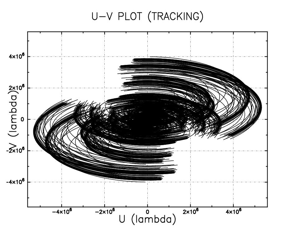
(b) UV track for $L_{Z}\neq 0$

Figure 6: UV tracking for Australian SKA proposed antennas/stations locations for declination = $-30^{o}$

We finish by stating some useful definitions and remarks. The earth’s axis determines half planes with the zenith and the source respectively. The angle between these two planes is called the hour angle. The angular distance of a source above or below the celestial equator is called its declination.

For good image quality, it is desirable that we sample as many points on the UV-plane as possible. As the earth rotates, the UV-points trace out curves on the UV-plane, populating it. This technique of making use of the earth’s rotation to fill up the sampling plane is called aperture synthesis. Naturally, we require that over time, the UV-plane is filled up as much as possible.

It is a useful exercise to work out the curve traced by a UV-point as the earth rotates. In particular, one will observe that the curve traced for a source at 0 declination is a straight line, that for $90^{\circ}$ declination is a circle, while all intermediate sources trace out ellipses of increasing eccentricity.

While different sources would require different UV distributions, it has been suggested that (i) in case of a dense UV plane, a Gaussian distribution is preferred in the radial direction, and a uniform distribution is preferred across the azimuth; (ii) in case of a sparse UV plane, a uniform distribution over the plane is preferred [2] .

Appendix B Area Under the Gaussian

Consider a Gaussian $y=ae^{-\frac{x^{2}}{2\sigma^{2}}}$ centered at $x=0$, amplitude $a$ and variance $\sigma^{2}$. Denote by $A$ the area under the curve: $A=a\int_{-\infty}^{\infty}e^{-\frac{x^{2}}{2\sigma^{2}}}dx$. Then, $A^{2}=a^{2}\big{\{}\int_{-\infty}^{\infty}e^{-\frac{x^{2}}{2\sigma^{2}}}dx\big{\}}^{2}$. Or, $A^{2}=a^{2}\int_{-\infty}^{\infty}\int_{-\infty}^{\infty}e^{-\frac{x^{2}+y^{2}}{2\sigma^{2}}}dxdy$.

Writing it in polar coordinates, we get $A^{2}=a^{2}\int_{0}^{2\pi}d\theta\int_{0}^{\infty}e^{-\frac{r^{2}}{2\sigma^{2}}}rdr$. This evaluates to $2\pi a^{2}c^{2}$. Therefore, $A=\sqrt{2\pi}ac$.

References

- [1] F. Boone, Interferometric Array Design: Optimizing the Locations of the Antenna Pads. Astronomy and Astrophysics, 377:368-376, 2001.
- [2] F. Boone, Interferometric Array Design: Distribution of Fourier Samples for Imaging. Astronomy and Astrophysics, 386:1160-1171, 2002.
- [3] B. F. Burke and F. Graham-Smith, Introduction to Radio Astronomy. Cambridge University Press, 2002.
- [4] C. Carilli and S. Rawlings (Eds), Science with the Square Kilometre Array. New Astronomy Reviews, Vol. 48, Elsevier, December 2004.
- [5] J. N. Chengalur, Y. Gupta and K. S. Dwarakanath (Eds), Low Frequency Radio Astronomy, 3rd edition. 2007.
- [6] T. J. Cornwell, A Novel Principle for Optimization of the Instantaneous Fourier Plane Coverage of Correction Arrays. IEEE AP-S Trans, 36(8):1165-1167, 1988.
- [7] M. de Villiers, Interferometric Array Layout Design by Tomographic Projections. Astronomy and Astrophysics, 469:793–797, 2007.
- [8] A. Karastergiou, R. Neri and M.A. Gurwell, Adapting and Expanding Interferometric Arrays. Astrophysical Journal Supplement Series, 164(2):552–558, 2006.
- [9] C.J. Lonsdale and R.J. Cappallo, Concepts for Large-N SKA. Perspectives on Radio Astronomy: Technologies for Large Antenna Arrays, 1999.
- [10] B. E. Cohanim, J. Hewitt and O. De Weck, The Design of Radio Telescope Array Configurations Using Multiobjective Optimization: Imaging Performance versus Cable Length. Astrophysical Journal Supplements Series, 154:705–719, 2004.
- [11] R. A. Perly, F. R. Schwab and A. H. Bridle (Editors), Synthesis Imaging–Course Notes from an NRAO Summer School held in Scorro, Mexico. August, 1985.
- [12] M. Ryle, D. Vonberg, Observations from the first multi-element astronomical radio interferometer. Solar radiation on 175Mc/s, Nature 158:339–340, 1946.
- [13] Y. Su, R. D. Nan and B. Peng, A New Method for Optmizing the Configuration of the Chinese Square Kilometer Array. Chinese Journal of Astronomy and Astrophysics, 4(2):198–204, 2004.
- [14] H. Takeuchi et al, Staged Deployment of the International Fusion Materials Irradiation Facility (IFMIF). In Proceedings of 18th Fusion Energy Conference, Italy, October 2000, IAEA-CN-77/FTP2/03.
- [15] N. C. Treloar, Investigation of Array Configurations for An Aperture Synthesis Radio Telescope. Journal of Royal Astronomical Society of Canada, 83(2):92–104, 1989.