SAXSFit: A program for fitting small-angle x-ray and neutron scattering data

Abstract

SAXSFit is a computer analysis program that has been developed to assist in the fitting of small-angle x-ray and neutron scattering spectra primarily from nanoparticles (nanopores). The fitting procedure yields the pore or particle size distribution and eta parameter for one or two size distributions (which can be log-normal, Schulz, or Gaussian). A power-law and/or constant background can also be included. The program is written in Java so as to be stand-alone and platform-independent, and is designed to be easy for novices to use, with a user-friendly graphical interface.

I Introduction

Small-angle x-ray scattering (SAXS) and small-angle neutron scattering (SANS) are well-established and widely used techniques for studying inhomogeneities on length scales from near-atomic scale (1 nm) up to microns (1000 nm). Recently, there has been an increasing emphasis and importance of nanoscale materials, due to the distinct physical and chemical properties inherent in these materials Pedersen2002 ; Frazel2003 . This, together with the significant advances in X-ray and neutron sources, has resulted in the dramatically increased use of SAXS and SANS for characterizing nanoscale materials and self-assembled systems. For example, these techniques are used to investigate polymer blends, microemulsions, geological materials, bones, cements, ceramics and nanoparticles. These measurements are often made over a range of length scales and in real time during materials processing or other reactions such as synthesis. However, there has been less progress in SAXS and SANS data analysis, although some analysis software is available. For example, programs based on IGOR Pro primarily for the reduction and analysis of SANS and ultra-small-angle neutron scattering (USANS) are available from NIST Kline2006 . PRINSAS has been developed for the analysis of SANS, USANS and SAXS data for geological samples and other porous media Hinde2004 . PRIMUS and ATSAS 2.1 are used primarily for the analysis of biological macromolecules in solutions, but can be used for other systems such as nanoparticles and polymers Konarev2003 ; Konarev2006 . FISH is another SANS and USANS fitting program developed at ISIS Heenan2007 . The Indra and Irena USAXS data reduction and analysis package developed at APS Ilavsky2008 is also based on IGOR. Both of these latter programs offer several advanced features, including multiple form factor choices and background reduction routines. While these programs provide a powerful analysis capability, they can be complicated to use and some are based on commercial software. This has motivated the development of a simple, easy to use analysis package.

In this paper, we describe SAXSFit - a program developed to fit SAXS and SANS data for systems of particles or pores with a distribution of particle (pore) sizes. SAXSFit is easy to use and applicable to a wide variety of materials systems. The program is most appropriate to low concentrations of particles or pores, due to the approximations used, but it does account for interparticle scattering within the local monodisperse approximation Pedersen1994 . The program is based on Java and is readily portable with a user-friendly graphical interface. The emphasis of SAXSFit is to provide an easy-to-use analysis package primarily for novices, but also of use to experts.

II Software description and use

SAXSFit is written in Java (SDK 1.4.2) and provides a graphical user interface (Figure 1) to select and adjust parameters to be used in the fit, change the plotting display and range of data to be used, calculating ‘initial guess’ patterns and running the fit. It uses the algorithms of a Matlab-based program Li2004 . The advantage of using Java is to provide a stand-alone program which is platform-independent, along with having a user-friendly graphical interface. SAXSFit is also available as a Windows executable.

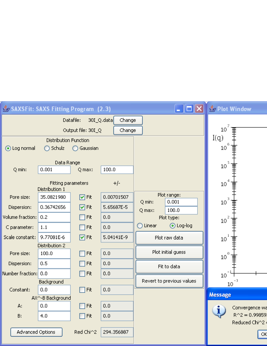
Figure 1: Screen dump of the SAXSFit graphical user interface and plot window.

SAXSFit can read ASCII data files (comma, space, or tab delimited), with or without a non-numerical header, which consist of two column ($q$, $I(q)$) or three-column ($q$, $I(q)$, error bars) data. Any subsequent columns in the data file are ignored. Once a data curve is successfully imported from an input file, it is plotted in a separate window and the fitting buttons are enabled. The error bars are also plotted if the input file contains them. The plot can be manipulated by changing the $q$-range and selecting whether it is log-log or linear. Initial guess and fitted curves are displayed when they are calculated. The $q$-min and $q$-max values of the data to be fitted are also shown as vertical lines and can be altered by changing the appropriate text boxes. Several fitting parameters are available, with the option to fit or fix their values.

Three distributions of particle/pore sizes are available: log-normal, Schulz and Gaussian. These use the same two fitting parameters, ‘particle/pore size’ ($r_{0}$) and ‘dispersion’ ($\sigma$), and are detailed in Section III.1. The units for the pore size are the inverse of the units of the data (i.e. Å for data in Å^-1, or nm for data in nm^-1). A second size distribution can also be included in the fit. It has been shown that the choice of distribution function does not dramatically affect the final result Caponetti1993 ; Kucerka2004 . A constant background and/or power law $Aq^{-B}$ can also be included.

Advanced options include the ability to change the maximum number of iterations and the weighting of the data. Again there are several options: a constant weighting ($w=1$), statistical weighting ($w=1/I(q)$), or uncertainty weighting ($w=1/\Delta I(q)^{2}$ - only applicable where data error bars ($\Delta I(q)$) have been imported).

Two output files are produced, consisting of the fit (a two-column ASCII file) and a log file (plain text) showing the values of the parameters at each iteration of the fitting process, and the final result including parameter uncertainties, reduced $\chi^{2}$ and goodness of fit ($R^{2}$ value). These are described in more detail in Section III.5. The final parameters are also displayed on the control panel.

Users must be aware of the assumptions made in the modeling of the data, which uses a hard sphere model with a local monodisperse approximation. Strongly interacting systems, for example systems with a high degree of periodicity, are outside the scope of this approximation. The user is responsible for understanding the applicability of this approximation to their system, and ensuring that the fitted results are physically meaningful.

III Mathematical details

The small angle scattering intensity $I(q)$ is related to the scattering cross section $\frac{d\sigma}{d\Omega}(q)$ by

$$I(q)=\phi_{0}At(\Delta\Omega)\frac{d\sigma}{d\Omega}(q)$$ (1)

where $\phi_{0}$ is the incident flux (number of photons, or neutrons, per area per second), $A$ is the illuminated area on the sample, $t$ is the sample thickness and $\Delta\Omega$ is the solid angle subtended by a pixel in the detector GlatterKratky1982 .

For SAXS, the scattering cross-section is calculated from the structure factor and particle/pore size distribution from

$$\frac{d\sigma}{d\Omega}(q)=r_{e}^{2}(\Delta\rho)^{2}N\int_{0}^{\infty}n(r)\left[f(qr)\right]^{2}S(qr)dr$$ (2)

where $r_{e}$ is the electron radius, $\Delta\rho$ is the electron density contrast, $N$ is the number density, $n(r)$ is the number fraction particle/pore size distribution (normalized so that the integral over $r$ is unity), $f(qr)$ is the spherical form factor, and $S(qr)$ is the structure factor. These terms are defined in the following sections. The final equation for the intensity used by the program is

$$I(q)=c\int_{0}^{\infty}n(r)\left[f(qr)\right]^{2}S(qr)dr$$ (3)

where the scale factor $c$ is a fitted parameter, equivalent to

$$c=\phi_{0}At(\Delta\Omega)r_{e}^{2}(\Delta\rho)^{2}N$$ (4)

For SANS an expression similar to Eq. 4 holds.

The data are modeled using a hard-sphere model with local monodisperse approximation Pedersen1994 . This model assumes that the particles are spherical and locally monodisperse in size. In other words, the particle positions are correlated with their size. This is a good approximation for systems with large polydispersity and the approximation provides meaningful results providing the particles are for the most part not inter-connected (e.g., the particle concentration is not too high) and are not spatially periodic. For porous systems (with not too high pore concentration), the ‘particle’ radius is equivalent to the pore size.

III.1 Particle/pore size distribution, $n(r)$

The user has the choice of three pore/particle size distributions, which use the same fitting parameters $r_{0}$ (‘pore size’ radius) and $\sigma$ (‘dispersion’). If two size distributions are selected, the distribution function is expanded to have the form:

$$n(r)=(1-\lambda)n_{1}(r,r_{0,1},\sigma_{1})+\lambda n_{2}(r,r_{0,2},\sigma_{2})$$

where $\lambda$ is the number fraction of the second distribution and $r_{0,j}$ and $\sigma_{j}$ are the $r_{0}$ and $\sigma$ parameters for the $j^{th}$ distribution. For example, a 50:50 mixture by number fraction would have $\lambda=0.5$. To model a situation involving a mixture with differing contrasts, $\lambda$ would be weighted by the different contrast values. The user has a choice of three distributions, as follows.

III.1.1 Log normal distribution

$$n(r)=\exp\left(-\frac{1}{2}\frac{\left[\ln\left(\frac{r}{r_{0}}\right)\right]^{2}}{\sigma^{2}}\right)\cdot\frac{1}{r\sigma\sqrt{2\pi}}$$

This has a maximum at $r=r_{0}\exp\left(-\sigma^{2}\right)$, a mean of $r_{0}\exp\left(\frac{-\sigma^{2}}{2}\right)$, and variance $r_{0}^{2}\left[\exp\left(2\sigma^{2}\right)-\exp\left(\sigma^{2}\right)\right]$.

III.1.2 Schulz distribution

$$n(r)=Z^{Z}X^{Z-1}\frac{\exp(-ZX)}{r\Gamma(Z)}$$

where $Z=\frac{1}{\sigma^{2}}$, $X=\frac{r}{r_{0}}$, and $\Gamma(Z)$ is the Gamma function, defined $\forall x\in\mathbf{R}$ by $\Gamma(x+1)=x\Gamma(x)$, and $\Gamma(1)=1$ Lau2004 . The Schulz distribution is frequently used in SANS analysis. It is physically reasonable in that it is skewed towards large sizes and has a shape close to a log-normal distribution. As $Z\rightarrow\infty$ it approaches a Gaussian distribution Bartlett1992 .

III.1.3 Gaussian distribution

$$n(r)=\frac{1}{\sigma\sqrt{2\pi}}\exp\left[-\frac{1}{2}\left(\frac{r-r_{0}}{\sigma}\right)^{2}\right]$$

The Gaussian distribution is symmetric about the mean, $r_{0}$, and has variance $(r_{0}\sigma)^{2}$. In practise it is only useful for systems with low polydispersity (small $\sigma$).

III.2 Spherical form factor, $f(qr)$

The spherical form factor has the following form Pedersen1994 ; Kinning1984 :

$$f(qr)=r\pi r^{3}\left[\frac{\sin(qr)-\cos(qr)qr}{(qr)^{3}}\right]$$

III.3 Structure factor, $S(qr)$

The structure factor follows the local monodisperse approximation (LMA) for hard spheres Pedersen1994 ; Huang2002 , given by

$$S(qR_{HS})=[1+24\eta G(qR_{HS})/(qR_{HS})]^{-1}$$

where $\eta$ is the dimensionless parameter eta (sometimes referred to as the hard sphere volume fraction, having a value between 0 and 1), $R_{HS}$ is the hard sphere pore/particle radius, defined as $R_{HS}=Cr$, where $C$ relates the hard-sphere radius to the physical particle radius Pedersen1994 , and $G(qR_{HS})$ has the form:

$$G(A)=\alpha(\sin A-A\cos A)/A^{2}+\\ \beta[2A\sin A+(2-A^{2})\cos A-2]/A^{3}+\\ \gamma(-A^{4}\cos A+4[(3A^{2}-6)\cos A+\\ (A^{3}-6A)\sin A+6])/A^{5}\\$$ (5)

where

$$\alpha =\frac{(1_{2}\eta)^{2}}{(1-\eta)^{4}}$$

$$\beta =-6\eta\frac{(1+\eta/2)^{2}}{(1-\eta)^{4}}$$

$$\gamma =\eta\alpha/2$$

When a second size distribution is included in the fit, it has the same $C$-parameter and $\eta$ values as the first distribution. To set the structure factor to unity, one simply sets $\eta=0$. This is appropriate for dilute systems.

III.4 Fitting routine details

The program uses a least-squares fitting routine which follows the Levenberg-Marquardt non-linear regression method to minimize the reduced $\chi^{2}$. The integrals are calculated using the Romberg integration method with $2^{10}$ intervals. Since the integral 1 must have finite bounds on $r$, these are chosen based on the range of the distribution function $n(r)$, such that $n(r)<1\times 10^{-15}$. The bounds are calculated numerically as follows:

For the log-normal and Schulz distributions, the lower bound is $r_{0}\exp(-8\sigma)$ and the upper bound $r_{0}\exp(8\sigma)$.

For the Gaussian distribution, the lower bound is the maximum of zero or $r_{0}-8\sigma$, and the upper bound is $r_{0}+8\sigma$.

III.5 Statistical analysis

The reduced $\chi^{2}$ and $R^{2}$ (goodness of fit) from the non-linear regression are reported at the end of the fitting procedure. These are common statistical measures and defined as follows:

$$\mathrm{Reduced}\phantom{a}\chi^{2}=\frac{1}{n-p}\sum_{i}w_{i}\left(y_{i}-F(x_{i})\right)^{2}$$

where $n$ is the number of data points, $p$ is the number of free parameters, $w_{i}$ are the weightings, $y_{i}$ is the input data $I(q)$ and $F(x)$ is the calculated $I(q)$.

$$R^{2}=1-\frac{\sum_{i}\left(y_{i}-F(x_{i})\right)^{2}}{\sum_{i}\left(y_{i}-\overline{F(x)}\right)^{2}}$$

where $y_{i}$ and $F(x_{i})$ are defined above, and $\overline{F(x)}$ is the average of the $F(x)$ values (a constant).

The parameter uncertainties are obtained by calculating the covariance matrix $C_{ij}$, from

$$C=(J^{T}WJ)^{-1}$$

where $J$ is the Jacobian matrix of partial derivatives and $W$ is a diagonal matrix where $W_{ii}$ is the weighting on the $i^{th}$ data point Toby2004 . Finally the reported parameter uncertainties are twice the square root of the diagonals of $C,$ i.e. $\delta P_{i}=2\sqrt{C_{ii}}$. This is two standard deviations, which for a Gaussian distribution of errors represents a 95% confidence interval.

IV Examples

Figure 2 shows examples of data and the fitted result for nanoporous methyl silsesquioxane films Huang2002 , formed by spin-coating a solution of the silsesquioxane along with a sacrificial polymer (‘porogen’), and then annealing to remove the polymer and leave behind a nanoporous network. As the proportion of porogen is increased, the pores are observed to increase in size Huang2002 . Data are shown for films with porogen loadings of 5 to 25 % with the background (from methyl silsesquioxane) subtracted. A single log-normal size distribution was fitted to each, the $C$-parameter was fixed at 1.1, $\eta$ was fixed to the porosity (as determined from the porogen loading), and no background function was used. The results obtained are given in Table 1 and show an increase in the pore size with increased porogen loadings, in good agreement with electron microscopy and previous results Huang2002 .

Figure 2: Examples of data from nanoporous silsesquioxane films, with different porogen loadings. Open symbols: raw data. Lines: fitted curves using SAXSFit.

Porogen loading	5%	10%	15%	25%
Pore size radius (Å)	18.77 $\pm$ 0.14	16.94 $\pm$ 0.06	22.42 $\pm$ 0.05	31.67 $\pm$ 0.06
Dispersion	0.305 $\pm$ 0.004	0.382 $\pm$ 0.002	0.367 $\pm$ 0.001	0.370 $\pm$ 0.001
Reduced $\chi^{2}$	1.105	2.117	2.913	2.023
$R^{2}$ (degree of fit)	0.9771	0.9858	0.9952	0.9976

Table 1: Fitted parameters for nanoporous silsequioxane film samples shown in Figure 2. The pore radii differ from that reported by Huang et al. Huang2002 due to a slightly different form used for the log-normal distribution. When plotted as a function of radius the distributions needed to fit the data are identical.

Figure 3 shows data from a nanoporous glass using a three arm star shaped polymer as the porogen Hedrick2002 , which was found to exhibit two pore size distributions.

Figure 3: Example of data from nanoporous glass, showing two pore size distributions. Open symbols: raw data. Line: fitted curve using SAXSFit.

The parameters for the fit are as follows:

First distribution: $r_{0}=50.5\pm 0.5,\sigma=0.287\pm 0.008$.

Second distribution: $r_{0}=15\pm 1,\sigma=0.23\pm 0.05$.

The number fraction of the second distribution was 88 $\pm$ 2 %, which equates to a volume of 16 $\pm$ 5 %. The parameter $\eta$ was the same for both distributions ($\eta=0.18\pm 0.01$) and the $C$-parameter was fixed at 1.1 for both distributions. The $R^{2}$ value was 0.9951 and reduced $\chi^{2}$ 3.33.

V Software availability and system requirements

SAXSFit is provided as a Windows executable (tested on Windows 98, 2000 and XP), or Java .jar executable (tested on Linux Ubuntu and Mac OS X10.4). The SAXSFit programs and user manual are available from http://www.irl.cri.nz/SAXSfiles.aspx .

VI Summary

SAXSFit is a useful program for fitting small angle x-ray and neutron scattering data, using a hard sphere model with local monodisperse approximation. SAXSFit provides an easy-to-use analysis package for novices and experts. It is stand-alone software and can be used in a variety of software environments.

- (1) P. Frazel; J. Appl. Cryst. 36 (2003) 397.
- (2) J. S. Pedersen; Neutrons, X-rays and Light Scattering, P. Linder and T. Zemb (eds.), Amsterdam, North Holland (2002) pp. 127-144.
- (3) S. R. Kline; J. Appl. Cryst. 39 (2006) 895.
- (4) A. L. Hinde; J. Appl. Cryst. 37 1020.
- (5) P. V. Konarev, V. V. Volkov, A. V. Sokolava, M. H. J. Koch and D. I. Svergun; J. Appl. Cryst. 36 (2003) 1277.
- (6) P. V. Konarev, M. V. Petoukhov, V. V. Volkov and D. I. Svergun; J. Appl. Cryst. 39 (2006) 277.
- (7) R. K. Heenan; http://www.isis.rl.ac.uk/LargeScale/ LOQ/FISH/FISH_intro.htm
- (8) J. Ilavsky; http://usaxs.xor.aps.anl.gov/staff/ilavsky/ irena.html
- (9) J. S. Pedersen; J. Appl. Cryst. 27 (1994) 595.
- (10) H. Li; Masters Project Report, Department of Chemical and Materials Engineering, San Jose State University, U.S.A.
- (11) E. Caponetti, M. A. Floriano, E. Di Dio and R. Triolo; J. Appl. Cryst. 26 (1993) 612.
- (12) N. Kucerka, M. A. Kiselev and P. Balgavy; Eur. Biophys. J. 33 (2004) 328.
- (13) O. Glatter and O. Kratky; Small Angle X-ray Scattering. Academic Press, London (1982).
- (14) H. T. Lau; A Numerical Library in Java for Scientists and Engineers. CRC Press, Boca Raton (2004).
- (15) P. Bartlett and R. H. Ottewill; J. Chem. Phys. 96 (1992) 3306.
- (16) D. J. Kinning and E. L. Thomas; Macromolecules 17 (1984) 1712.
- (17) E. Huang, M. F. Toney, W. Volksen, D. Mecerreyes, P. Brock, H. C. Kim, C. J. Hawker, J. L. Hedrick, V. Y. Lee, T. Magbitang, R. D. Miller, and L. B. Lurio; Appl. Phys. Lett. 81 (2002) 2232.
- (18) B. H. Toby and S. J. L. Billinge; Acta Cryst. A 60 (2004) 315.
- (19) J. L. Hedrick, T. Magbitang, E. F. Connor, T. Glauser, W. Volksen, C. J. Hawker, V. Y. Lee and R. D. Miller; Chem. Eur. J. 8 (2002) 3308.