Magnetic reconnection and topological trigger in physics of large solar flares

Abstract

Solar flares are accessible to a broad variety of observational methods to see and investigate the magnetic reconnection phenomenon in high-temperature strongly-magnetized plasma of the solar corona. An analysis of the topological peculiarities of magnetic field in active regions shows that the topological trigger effect is necessary to allow for in order to construct models for large eruptive flares.

The topological trigger is not a resistive instability which leads to a change of the topology of the field configuration from pre- to post reconnection state. On the contrary, the topological trigger is a quick change of the global topology, which dictates the fast reconnection of collisional or collisionless nature.

The current state of the art and development potential of the theory of collisionless reconnection in the strong magnetic fields related to large flares are briefly reviewed. Particle acceleration is considered in collapsing magnetic traps created by reconnection. In order to explain the formation of coronal X-ray sources, the Fermi acceleration and betatron mechanism are simultaneously taken into account analytically in a collisionless approximation. Finally, the emphasis is on urgent unsolved problems of solar flare physics.

1 The role of magnetic fields in flares

1.1 Basic questions

Frequent observations of solar flares became available in the 1920s. Early studies showed that flares were associated with magnetic fields. Estimates of the energy required to power large flares led to the conclusion that flares must be electromagnetic in origin. Step by step it became more clear that a flare is the result of reconnection of magnetic fields. However there were some objections to the hypothesis that the energy of a flare could be stored in the form of a magnetic field of reconnecting current layers (RCLs).

(1) It was claimed that measurements of photospheric magnetic fields do not demonstrate an unambiguous relation between flares and the changes of the fields. More exactly, the changes in question are those that occur immediately before a flare to create it. These changes were supposed to be the cause of a flare.

(2) Next objection was related to the time of dissipation of the magnetic field in a volume that would contain the energy necessary for a flare. If this time is estimated in a usual way as the diffusion time in a solar plasma of a finite conductivity, then it is too long compared with the observed duration of a flare.

(3) The third objection was the most crucial one: the observers had never seen real RCLs in solar flares.

Starting from Severny [1], solar observers have been studying flare-related changes in photospheric magnetic fields to provide information how an active region (AR) stores and releases its energy (see Lin et al. [2], Wang [3]). However the role of photospheric fields is still an area of ongoing research (Section 1.3). What are the answers of the reconnection theory to the objections listed above?

1.2 Concept of magnetic reconnection in solar flares

According to contemporary views, the principal flare process is contingent on the accumulation of the free magnetic energy in the corona. By ‘free’ we mean the surplus energy above that of a potential magnetic field

$$B_{\alpha}({\bf r})=\,\frac{\partial\psi}{\partial r_{\alpha}}\,.$$ (1)

Here $\psi({\bf r})$ is the potential of the field, the index $\alpha=1,2,3$. The potential field has the sources (sunspots, background fields) in the photosphere.

The free magnetic energy is related to the electric currents in the corona. A solar flare corresponds to rapid changes of these currents. So we distinguish between two processes: a slow accumulation of energy and its fast release, a flare.

Figure 1: The classical 2D cartoon of magnetic reconnection in a solar flare. Three states of the field: (a) the initial one, (b) the pre-reconnection state, (c) the final state after reconnection.

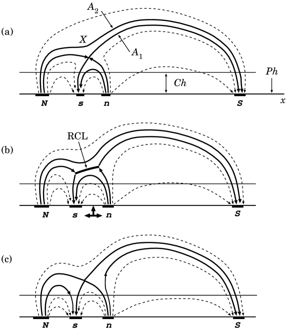
Let us see them in a classical example, the evolution of the quadrupole configuration of sunspots (Figure 1). The sunspots of pairwise opposite polarity are shown: $N$ and $S$ represent a bipolar group of sunspots in an AR, $n$ and $s$ model a new emerging flux. All sunspots are placed along the axis $x$ in the photospheric plane $Ph$ at the bottom of the chromosphere $Ch$.

The field line $A_{1}$ in Figure 1a is the separatrix line of the initial state (a), this line will reconnect first. $X$ is the zeroth point of the field at the initial state, here the RCL is created at the state (b). The field line $A_{2}$ is the separatrix of the final state (c) or the last reconnected field line. Therefore $\delta A=A_{2}-A_{1}$ is the reconnected magnetic flux.

Three solid arrows under the photosphere $Ph$ in Figure 1b show a slow emergence of a new magnetic flux (the sunspots $n$ and $s$). The sunspots have been emerged but the field lines do not start to reconnect. More exactly, they reconnect too slowly because of high conductivity of plasma in the corona. In the first approximation, we neglect this reconnection.

In general, the redistribution of fluxes appears as a result of the slow changes of the field sources in the photosphere. These changes can be either the emergence of a new flux from below the photosphere (Figure 1) or other flows of photospheric plasma, in particular the shear flows, inhomogeneous horizontal flows along the neutral line of the photospheric magnetic field. For this reason, an actual (slow and fast) reconnection in the corona is always a three-dimensional (3D) phenomenon (Section 2).

1.3 Some new results of the magnetic field observations

Let us come back to objection (1) in Section 1.1 to the reconnection theory of flares. According to the theory, the free energy is related to the current $J$ inside the RCL. A flare corresponds to rapid changes of this current. However the magnetic flux through the photosphere $Ph$ (Figure 1) changes only little over the whole area of a flare during this process, except in some particular places, for example, between close sunspots $N$ and $s$.

Sunspots in the photosphere are weakly affected by a flare because the plasma in the photosphere is almost $10^{9}$ times denser than the plasma in the corona. It is difficult for disturbances in the tenuous corona to affect the extremely massive plasma in the photosphere. Only small perturbations penetrate into the photosphere.

The same is true in particular for the vertical component of the field. The photospheric magnetic field changes a little during a flare over its whole area. As a consequence, after a flare the large-scale structure in the corona can remain free of noticeable changes, because it is determined mainly by the potential part of the field above the photosphere. More exactly, even being disrupted, the structure will come to the potential configuration corresponding to the post-flare position of the photospheric sources.

On the other hand, in the “Bastille-day” flare on 2000 July 14 and in some other large flares, it was possible to detect the real changes in a sunspot structure just after a flare. The outer penumber fields became more vertical due to reconnection in the corona during a flare (Liu et al. [4], Wang et al. [5]). One can easily imagine such changes by considering Figure 1 between sunspots $N$ and $s$.

Sudol and Harvey [6] used the magnetograms to characterize the changes in the vertical component of photospheric field during 15 large flares. An abrupt, significant, and persistent change occurred in at least one location within the flaring AR during each event after its start. Among possible interpretations, Sudoh and Harvey favor one in which the field changes result from the penumber field relaxing upward by reconnecting magnetic field above the photosphere. This interpretation is similar to than one given by Liu et al. [4] and Wang et al. [5].

As for objection (2) to the hypothesis of accumulation of energy in the form of magnetic field of current layers, the rapid dissipation of the field necessary for a flare is explained by the theory of super-hot turbulent-current layers (Section 4). In what follows, we advocate that the potential part of magnetic field in the solar corona determines a large-scale structure and properties of active regions, while the reconnecting current layers determine energetics and dynamics of flares.

2 Three-dimensional reconnection in flares

2.1 The first topological model of an active region

2.1.1 The potential field approximation

Gorbachev and Somov [7,8] have developed a 3D model for a potential field in the AR 2776 with an extended flare of 1980 November 5. Before discussing the AR and the flare (see Section 2.2), let us consider, at first, the general properties of this class of models called topological.

Figure 2: A model for the magnetic field of four sunspots of pairwise opposite polarity. The sunspots $N$ and $S$ in the photospheric plane $Ph$. The separatrices $S_{\rm 1}$ and $S_{\,\rm 2}$ cross at the separator $X_{\rm 1}XX_{\rm 2}$ above the plane $Q$ of the effective magnetic charges $e_{{}_{\rm N}}$, $e_{{}_{\rm S}}$, etc.

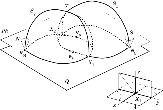
In the simplest model (Gorbachev and Somov [9]), four field sources – the magnetic “charges” $e_{{}_{\rm N}}$ and $e_{{}_{\rm S}}$, $e_{\rm n}$ and $e_{\rm s}$, located in the plane $Q$ under the photosphere $Ph$ (Figure 2) – are used to reproduce the main features of the observed field in the photosphere related to the four most important sunspots: $N,\,S,\,n$ and $s$. As a consequence, the quadrupole model reproduces only the large-scale features of the actual field in the corona related to these sunspots. As a minimum, the four sources are necessarily to describe two interacting magnetic fluxes having the two sources per each. The larger number of sources are not necessarily much better.

The main features are two magnetic surfaces called the separatrices: $S_{\rm 1}$ and $S_{\,\rm 2}$ (Figure 2). They divide the whole space above the plane $Q$ into four regions and, correspondingly, the whole field into four magnetic fluxes having different linkages. The field lines are grouped into four regions according to their termini. The separatrices are formed from lines beginning or ending at magnetic zeroth points $X_{1}$ and $X_{\,2}$. For example, the field lines originating at the point $X_{1}$ form a separatrix surface $S_{\rm 1}$.

The topologically singular field line $X_{\rm 1}XX_{\rm 2}$, lying at the intersection of the separatrices, belongs to all four fluxes (two reconnecting and two reconnected fluxes) that interact at this line, the 3D magnetic separator. So the separator separates the interacting fluxes by the separatrices. Detection of a separator, as a field line that connects two zeroth points in the Earth magnetotail, by the four Cluster spacecraft (Xiao et al. [10]) provides an important step towards establishing an observational framework of 3D reconnection.

2.1.2 Classification of zeroth points

Let us clarify properties of the zeroth points of the magnetic field discussed above. In the vicinity of a zeroth point ${X}_{i}$ located at ${\bf r}={\bf r}_{i}$ in the plane $Q$, the vector of field is represented in the form

$$B_{\alpha}({\bf r})=\,\frac{\partial\psi}{\partial r_{\alpha}}=M_{\alpha\beta}({\bf r}_{i})\,\xi_{\beta}\,.$$ (2)

Here $\psi({\bf r})$ is the potential of the field, the vector ${\bf\xi}={\bf r}-{\bf r}_{i}$, the index $i=1,2$ ; the Greek indices $\alpha,\beta=1,2,3$ . The symmetric matrix

$$M_{\alpha\beta}({\bf r}_{i})=\,\frac{\partial^{2}\psi\,({\bf r}_{i})}{\partial r_{\alpha}\,\partial r_{\beta}}=\left|\begin{array}[]{ccc}\lambda_{\,1}&0&0\\ 0&\lambda_{\,2}&0\\ 0&0&\lambda_{\,3}\end{array}\right|\,$$ (3)

in the frame of coordinates $r_{\alpha}^{\,\prime}$ related to the eigenvectors ${\bf e}_{\alpha}^{\,\prime}$, $\lambda_{\,\alpha}$ are the eigenvalues of the matrix. Because the field is potential, all the $\lambda_{\,\alpha}$ are real numbers. Positive eigenvalues $\lambda_{\,\alpha}$ correspond to the field lines emerging from a zeroth point and negative $\lambda_{\,\alpha}$ correspond to the lines arriving at a point ${\bf r}_{i}$.

If the determinant

$${\rm det}\,M_{\alpha\beta}({\bf r}_{i})=\lambda_{\,1}\,\lambda_{\,2}\,\lambda_{\,3}\neq 0\,,$$ (4)

then the zeroth point is called non-degenerate. Such a point is isolated, i.e., the magnetic field in its vicinity does not vanish. Since ${\rm div}\>{\bf B}=0$, we obtain a condition

$$\lambda_{\,1}+\lambda_{\,2}+\lambda_{\,3}=0\,.$$ (5)

Therefore there exist only three following classes of zeroth points.

Type A. All eigenvalues $\lambda_{\,\alpha}\neq 0$. This corresponds to two zeroth points shown in Figure 2. At the first one $X_{\,1}$

$$\lambda_{\,1}<0\,,\quad\lambda_{\,2}>0\,,\quad\lambda_{\,3}>0\,.$$ (6)

Using the analogy with fluid flow, we say that field lines “flow in” along the $x$ axis and “flow out” along the separatrix plane $(y,z)$ as shown in the left bottom insert in Figure 2. We shall call this subclass of non-degenerate zeroth point as the Type A$-$ since $\lambda_{\,1}<0\,$.

On the contrary, at the point  $X_{\,2}$

$$\lambda_{\,1}>0\,,\quad\lambda_{\,2}<0\,,\quad\lambda_{\,3}<0\,.$$ (7)

This will be the Type A+ since $\lambda_{\,1}>0\,$.

Type B. This is a degenerate case

$$\lambda_{\,1}=-\lambda_{\,2}\neq 0\,,\quad\lambda_{\,3}=0\,.$$ (8)

It can occur, for example, if a zeroth point belongs to a neutral line, i.e. a line consisting of zeroth points of the hyperbolic type.

Type C. This is another degenerate case

$$\lambda_{\,1}=\lambda_{\,2}=\lambda_{\,3}=0\,.$$ (9)

It means that three neutral lines intersect at the point ${\bf r}_{i}$ .

2.1.3 The number of zeroth points

In order to use some general theorems of differential geometry, we have to smooth the point charges of magnetic field. The smoothed potential $\psi$ of a positive source has a maximum at the point where this charge is located. Hence at this point all eigenvalues $\lambda_{\,\alpha}>0$. At a singular point with a negative charge, all $\lambda_{\,\alpha}<0$, and the potential has a minimum.

In order to establish a relation between the number of non-degenerate points, let us introduce the topological index

$$I_{top}\hskip 0.56905pt({\bf r}_{i})={\rm sign}\left[\,{\rm det}\,M_{\alpha\beta}({\bf r}_{i})\,\right]={\rm sign}\left(\,\lambda_{\,1}\,\lambda_{\,2}\,\lambda_{\,3}\,\right)\,.$$ (10)

Here the function ${\rm sign}\,(x)=+1$ if $x>0$ and ${\rm sign}\,(x)=-1$ if $x<0$. Thus the possible types of points have the indices presented in Table 1.

Table 1: Topological indices of singular and zeroth points

Type of a point	$\,\,I_{top}$
Maximum of potential $\psi$	$+1$
Minimum of potential $\psi$	$-1$
Zeroth point of Type A$+$	$+1$
Zeroth point of Type A$-$	$-1$

According to Dubrovin et al. [11] (see Part II, Ch. 3, § 14), with some difference in notations that are standard in physics, we formulate the following statement.

Theorem 1: For a 3D potential magnetic field, in a general 3D case of magnetic source location,

$$\sum_{i}\,I_{top}\hskip 0.28453pt({\bf r}_{i})=\frac{1}{4\pi}\int{\bf B}\left[\,\frac{\partial{\bf B}}{\partial\hskip 0.28453pt\theta}\,\times\frac{\partial{\bf B}}{\partial\varphi}\,\right]\,\frac{d\hskip 0.28453pt\theta\,d\varphi}{B^{3}}\,=J^{\,(3)}\,,$$ (11)

where the integral is taken over the sphere of infinite radius.

If the total magnetic charge

$$e_{\,tot}=\sum_{i}e_{i}>0\,,$$ (12)

then the integral $J^{\,(3)}=+1$. Let $N_{max}$ ($N_{min}$) is the number of maxima (minima) of the potential $\psi$ of magnetic field ${\bf B}$, $N_{A+}$ ($N_{A-}$) is the number of zeroth points of Type A$+$ (A$-$), then according to (11) we have

$$N_{max}-N_{min}+N_{A+}-N_{A-}=+1\,.$$ (13)

If $e_{\,tot}<0$ then $J^{\,(3)}=-1$, and we write $-1$ on the right-hand side of Equation (13).

If the total charge

$$e_{\,tot}=0\,,$$ (14)

then $J^{\,(3)}=0$, and the following relation is valid:

$$N_{max}-N_{min}+N_{A+}-N_{A-}=0\,.$$ (15)

For the magnetic field shown in Figure 2, $N_{max}=N_{min}=2$. Hence formula (15) gives us an equation

$$N_{A+}=N_{A-}\,$$ (16)

but not the total number of zeroth points, that we need.

However, if all the charges are located in the plane Q as illustrated by Figure 2, then we can obtain an additional information about the number of zeroth points, another equation. Let us determine the topological index for the 2D vector field in the same plane

$${\bf B}^{\,(2)}(x,y)=\left\{\,B_{x},B_{y}\,\right\}\,$$ (17)

following general definition from Dubrovin et al. [11]

$$I_{top}^{\,(2)}\hskip 0.56905pt({\bf r}_{i})={\rm sign}\left(\,\lambda_{\,1}\,\lambda_{\,2}\,\right)\,.$$ (18)

Hence the possible types of non-degenerate points have the indices presented in Table 2.

Table 2: Topological indices of singular and zeroth points of the 2D field in the plane $Q$

Type of a point	$\,\,I_{top}^{\,(2)}$
Maximum of potential $\psi$	$+1$
Minimum of potential $\psi$	$+1$
Zeroth point (a saddle)	$-1$

In this case of a plane arrangement of magnetic charges, we have to rewrite Theorem 1 as follows.

Theorem 2: For a potential magnetic field in the plane $Q$, in which the charges are located,

$$\sum_{i}\,I_{top}^{\,(2)}\hskip 0.28453pt({\bf r}_{i})=\frac{1}{2\pi}\int\left[\,{\bf B}^{\,(2)}(x,y)\,\right]^{-2}\,\left(\,B_{x}\,dB_{y}-B_{y}\,dB_{x}\,\right)\,=J^{\,(2)}\,.$$ (19)

Here the integral is taken over the circle of infinite radius in the positive direction of circulation.

For a plane field (17) of the dipole type (i.e., $e_{\,tot}=0$ and an effective dipole moment ${\bf m}\neq 0$) the integral $J^{\,(2)}=2$. Thus we have

$$N_{max}^{\,(2)}+N_{min}^{\,(2)}-N_{A}^{\,(2)}=2\,,$$ (20)

where $N_{max}^{\,(2)}$ ($N_{min}^{\,(2)}$) is the number of maxima (minima) of the potential $\psi=\psi(x,y,0)$ in the plane $z=0$, $N_{A}^{\,(2)}$ is the number of zeroth points, the saddles. Because of the symmetry relative to the plane $Q$, everywhere in the plane (outside of the charges) $B_{z}=0$. Therefore the saddles of the plane field are zeroth points of a 3D field.

For the field shown in Figure 2, $N_{max}^{\,(2)}=2$ and $N_{min}^{\,(2)}=2$. Hence, according to formula (20), the number of zeroth points $N_{A}^{\,(2)}=2$. By using Equation (16), we conclude that, in the simple case under consideration,

$$N_{A+}=N_{A-}=1\,.\quad\quad\quad\quad{\rm Q.e.d.}$$ (21)

2.1.4 The electric currents needed

The potential field model does not include any currents and so cannot model an energy stored in the fields and released in flares. Therefore here we introduce some currents and energetics to a flare model.

The topological model under consideration does not mean, of course, that we assume the existence of magnetic charges under the photosphere as well as the real zeroth points $X_{1}$ and $X_{\,2}$ in the plane $Q$ which does not exist either. We assume that above the photosphere the large-scale field can be described in terms of such a simple model. If the magnetic sources move and change, the field also changes. It is across the separator that the magnetic fluxes are reconnected so that the field could remain potential, if there were no plasma.

In the presence of a plasma of low resistivity, the separator plays the same role as the hyperbolic zeroth line of magnetic field, familiar from 2D MHD problems (Syrovatskii [12], Brushlinskii et al. [13], Biskamp [14,15]; see review of a current state of numerical simulations and laboratory experiments in Yamada et al. [16]. In particular, as soon as the separator appears, the electric field ${\bf E}_{\,0}$ induced by the varying magnetic field produces an electric current ${\bf J}$ along the separator. The current interacts with the potential field in such a way that the current assumes the shape of a thin wide current layer (RCL in Figure 3).

Figure 3: A schematic view of a RCL with a total current $J$ at the separator.

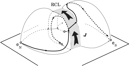
In a low-resistivity plasma the current layer hinders the redistribution of magnetic fluxes, their reconnection. This results in an energy being stored in the form of magnetic energy of a current layer – the free energy. Therefore the slowly-reconnecting current layer appears at the separator (Syrovatskii [17], Longcope and Cowley [18]) in a pre-flare stage. If for some reason (see Somov [19], Cassak et al. [20], Uzdensky [21]) reconnection becomes fast, the free magnetic energy is rapidly converted into energy of particles. This is a flare. The rapidly-reconnecting current layer, being in a high-temperature turbulent-current state (Section 4), provides the energy fluxes along the reconnected field lines.

Reconnection for 3D models without zeroth points in and above the photosphere, as we assumed in Figure 3, is qualitatively the same as the 2D reconnection in the models with a non-zero longitudinal magnetic field ${\bf B}_{\,\parallel}\,$. The inductive electric field along the separator is the driving force of reconnection. The field lines going to reconnect are pushed into the RCL and the lines coming out of the RCL are pulled by the longitudinal electric field. Thus reconnection in 3D should be taken to mean effects associated with the RCL, as in 2D (Greene [22], Lau and Finn [23]).

An actual 3D reconnection at a separator proceeds in the presence of an increasing (or decreasing) longitudinal field ${\bf B}_{\,\parallel}\,$. What factors do determine the increase (or decrease) of this field? - The first of them is the global field configuration, i.e. the relative position of the magnetic field sources in an AR. It determines the position of a separator and the value of the longitudinal field at the separator and in its vicinity. This field is not uniform, of course.

The second factor is evolution of the global configuration, more exactly, the electric field ${\bf E}_{\,0}$ related to the evolution and responsible for driven reconnection at a separator. The direction of reconnection - with an increase (or decrease) of the longitudinal magnetic field - depends on the sign of the electric field projection on the separator, i.e. on the sign of the scalar product $(\,{\bf E}_{\,0}\cdot{\bf B}_{\,\parallel}\,)$. In general, this sign can be plus or minus with equal probabilities, if there are no preferential configurations of the global field or no preferential directions of the AR evolution.

2.2 The solar flare on 5 November 1980

2.2.1 Observed and model magnetograms

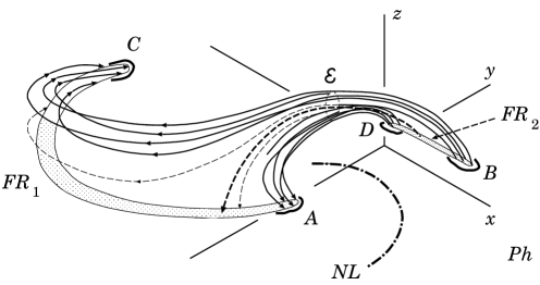
The first well-studied example was the extended 1B/M4 flare on 5 November 1980 (e.g. Rust and Somov [24]) observed by the satellite SMM (Figure 4).

Figure 4: The flare of 1980 November 5 as observed by SMM.

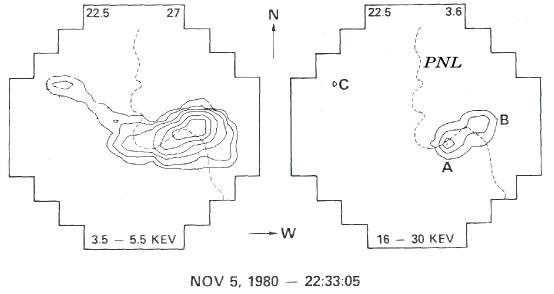
Three bright hard X-ray (HXR) kernels A, B and C are well distinguished in the right panel. The soft X-ray (SXR) elements of the flare, as seen in the left panel, consist presumably of two overlapping coronal loops, AB and BC. Their footpoints in the chromosphere have been identified as the sources of HXR and H$\alpha$ emission.

Figure 5: The line-of-sight component of magnetic field in AR 2776. Two flare ribbons observed in H$\alpha$ line are shown as shadow areas; $FR_{1}$ is the longer one.

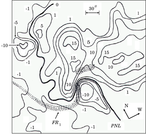
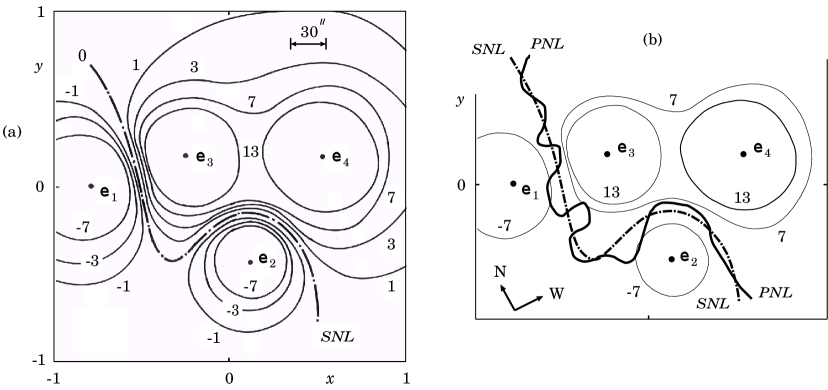
Figure 5 shows the line-of-sight magnetogram of the AR 2776 where the flare occurred. Numbers shows a magnitude of the field measured in $10^{2}$ G. Two narrow flare ribbons are shown on either side of the photospheric neutral line ($PNL$). Let us identify the four largest regions in which the field of a single polarity is concentrated: two of northern polarity and two of souther polarity. Since the AR is comparatively close to the center of the solar disk, the magnetogram represents the vertical component $B_{z}$ at the photospheric level fairly well.

Figure 6: The model magnetogram. (a) Positions and magnitudes of the sources fit the main features of the observed magnetogram. (b) The calculated simplified neutral line ($SNL$) approximates the observed photospheric neutral line ($PNL$).

Let us make a model of the magnetogram shown in Figure 5. With this aim, we calculate the vertical component $B_{z}$ of magnetic field in the photospheric plane $Ph$ (plane $z=0$ in this Section) in the potential approximation by using the simple formula

$${\bf B}\,(x,y,z)=\sum\limits_{i=1}^{4}\frac{e_{i}}{|\,{\bf r}-{\bf r}_{i}\,|^{\,2}}\times\frac{{\bf r}-{\bf r}_{i}}{|\,{\bf r}-{\bf r}_{i}\,|}\,.$$ (22)

Here $e_{i}$ are the effective charges of field, and ${\bf r}_{i}$ are their radius vectors:

$$\begin{array}[]{ll}e_{1}=-\,2.5\,,&{\bf r}_{1}=\{\,-\,0.8\,,0\,\,,-\,0.1\,\}\,;\\ e_{2}=-\,1.0\,,&{\bf r}_{2}=\{\,0.1\,,-\,0.4\,,-\,0.1\,\}\,;\\ e_{3}=+\,3.0\,,&{\bf r}_{3}=\{\,-\,0.25\,,0.15\,,-\,0.1\,\}\,;\\ e_{4}=+\,4.5\,,&{\bf r}_{4}=\{\,0.5\,,0.16\,,-\,0.1\,\}\,.\\ \end{array}$$

Note that the total magnetic charge

$$e_{\,tot}=4>0\,.$$ (23)

Thus, in order to determine a relation between the number of zeroth points and the numbers of field sources, we have to use formula (13). It gives us an equation

$$N_{A+}=N_{A-}+1\,.$$ (24)

We shall come back to this equation, considering a topological portrait of the AR.

The parameters $e_{i}$ and ${\bf r}_{i}$ have been selected in order to reproduce in an optimal way the fluxes of individual polarities in the photospheric plane (Figure 6a) as well the shape of the photospheric neutral line ($PNL$ in Figure 6b). The calculated simplified neutral line ($SNL$) smoothes the curve $PNL$ in small scales but conserves its $S$-type shape in a large scale, in the linear scale of the AR. In Figure 6, the length unit equals 150${}^{\,\prime\prime}\approx 1.1\times 10^{10}$ cm; the numbers near the curves show the values of the vertical component of the field measured in 10² G.

Because the simplest model uses a minimal number of magnetic sources – four, which is necessary to describe the minimal number of interacting fluxes – two, we call it the quadrupole-type model (Figure 6). This is not an exact definition (because in the case under consideration $e_{{}_{\rm N}}\not=-\,e_{{}_{\rm S}}$ and $e_{\rm n}\not=-\,e_{\rm s}$) but it is convenient for people who know the exact-quadrupole model (Sweet [25]). In fact, the difference, the presence of another separator in the model under consideration, is not small and can be significant for actual ARs. The second separator may be important to give accelerated particles a way to escape out of an AR in the interplanetary space.

We calculate the field lines integrating the ordinary differential equations

$$\frac{dx}{B_{x}}=\frac{dy}{B_{y}}=\frac{dz}{B_{z}}\,.$$ (25)

Here $(dx,dy,dz)$ is an arch element directed along a field line. The vector ${\bf B}$ is determined at each point by formula (22).

2.2.2 Topological portrait of the active region

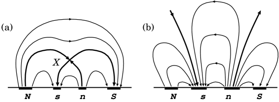
The topological properties of magnetic field are determined by the number and locations of zeroth points. In the case under consideration, there are three points in the plane $Q$ (here $z=-0.1$) shown in Figure 7. The coordinates of these points are:

$$\begin{array}[]{ll}{X}_{1}=\{\,-\,0.133\,,-\,0.739\,,-\,0.1\,\}\,,\\ {X}_{2}=\{\,0.076\,,\,0.179\,,-\,0.1\,\}\,,\\ {X}_{3}=\{\,-\,2.26\,,-\,0.439\,,-\,0.1\,\}\,.\\ \end{array}$$

Figure 7: The topological portrait of the AR 2776 where the extended 1B/M4 solar flare of 1980 November 5 occurred.

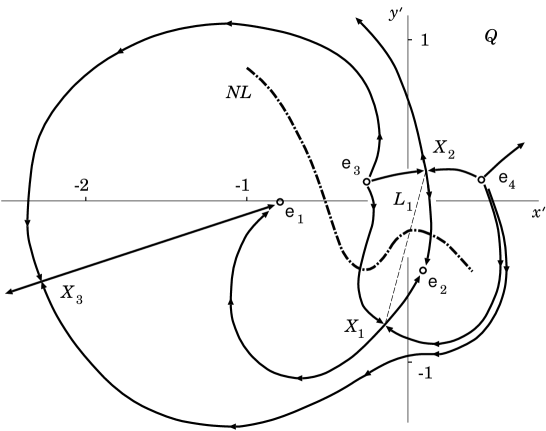
Figure 7 shows the topologically important field lines in the plane ($x^{\prime},y^{\prime}$) which is the plane $Q$ of the sources ${\rm e}_{1}$, ${\rm e}_{2}$, ${\rm e}_{3}$, and ${\rm e}_{4}$. Since the total charge $e_{\,tot}>0$, instead of Equation (20) for the number of zeroth points of 2D field (17), we have an equation

$$N_{max}^{\,(2)}+N_{min}^{\,(2)}-N_{A}^{\,(2)}=1\,,$$ (26)

because according to formula (19) we find the value $J^{\,(2)}=1$. It follows from (26) that the total number of zeroth points

$$N_{A}^{\,(2)}=3\,.$$ (27)

On the other hand,

$$N_{A}^{\,(2)}=N_{A+}+N_{A-}\,.$$ (28)

With account of (24) taken, we conclude that $N_{A+}=2$ and $N_{A-}=1$.

The field lines shown in Figure 7 play the role of separatrices and show the presence of two separators. Two points $X_{1}$ (Type $A_{+}$) and $X_{\,2}$ (Type $A_{-}$) are located in the vicinity of the magnetic sources and are connected by the first separator shown by its projection, the thin dashed line $L_{1}$. Near this main separator, the field and its gradient are strong and determine the flare activity of the AR.

Another separator starts from the point $X_{3}$ (the Type $A_{+}$) far away from the sources and goes much higher above the AR to infinity. The second separator can be responsible for flares in weaker magnetic fields and smaller gradients high in the corona. The second separator is also a good place for the particles accelerated along the main separator to escape from the AR in the interplanetary space.

We suppose that a part of the flare energy is released in some region ${\cal E}$ near the apex of the main separator. The energy fluxes $F_{{}_{\cal E}}$ propagate along the field lines connecting the energy source with the photosphere. Projections of the energy source ${\cal E}$ on the photospheric plane $Ph$ along the field lines are shown as two “flare ribbons” $FR_{1}$ and $FR_{2}$ in Figure 8. Therefore the model allows us to identify the flare brightenings, in the H$\alpha$ line as well as in EUV and HXRs, with the ribbons located at the intersection of the separatrices with the chromosphere which is placed slightly above the photospheric plane ($Ph$).

Figure 8: Potential field lines cross a region of primary energy release ${\cal E}$ situated at the apex of the main separator (boldface dashed curve). Two flare ribbons are formed where these lines cross the photospheric plane $Ph$.

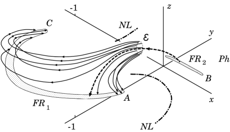
The characteristic saddle structure of the orthogonal (perpendicular to a separator) field ${\bf B}_{\bot}$ in the vicinity of the separator leads to a spatial redistribution of the energy flux $F_{{}_{\cal E}}$ of heat and accelerated particles. This flux is split apart in such a way that it creates the long-narrow ribbons. Thus, at first, the model had reproduced the observed features of the real solar flare. In particular, the model predicts the simultaneous flaring of the two chromospheric ribbons. Moreover it predicts that a concentration of the field lines that bring energy into the ribbons is higher at the edges of the ribbons, i.e. at relatively compact regions indicated as $A$, $B$, and $C$. Here the H$\alpha$ brightenings must be especially bright. This is consistent with observations of H$\alpha$ “kernels” in this flare.

2.3 Features of the flare topological model

Since in the kernels the energy fluxes are concentrated, the impulsive heating of the chromosphere creates a fast expansion of high-temperature plasma upwards into the corona (e.g. Somov [26]). This effect is known as the chromospheric “evaporation” observed in the EUV and SXR emission. Evaporation lights up the coronal loops in flares.

The topological model also shows that the flare ribbons as well as their edges with H$\alpha$ kernels are connected to a common source of energy at the separator (see ${\cal E}$ in Figure 9). Through this region all four kernels are magnetically connected to one another. Therefore the SXR loops look like they are crossing or touching each other.

Figure 9: Field lines that connect the H$\alpha$ kernels $A$, $B$, $C$, and $D$. Chromospheric evaporation creates a picture of the crossing SXR loops.

So the reconnecting magnetic fluxes are distributed in the corona in such a way that the two SXR loops may look like that they interact with each other. That is why such structures are usually considered as evidence in favor of a model of two interacting loops (Sakai and de Jager [27]). The difference, however, exists in the primary source of energy. High concentrations of electric currents and twisted magnetic fields inside the interacting loops are created by some under-photospheric dynamo mechanism. If these currents are mostly parallel they attract each other giving an energy to a flare (Gold and Hoyle [28]). On the contrary, according to the topological model, the flare energy comes from an interaction of magnetic fluxes that can be mostly potential.

The S-shaped structures observed in SXRs are usually interpreted in favour of non-potential fields. In general, the shapes of loops are signature of the helicity of their magnetic fields. The S-shaped loops match flux tubes of positive helicity, and inverse S-shaped loops match flux tubes of negative helicity (Pevtsov et al. [29]). However, in Figure 9, the S-shaped structure $C{\cal E}B$ connecting the bright points $C$ and $B$ results from the computation of the potential field.

In the AR 2776, Den and Somov [30] found a considerable shear of a potential field above the $PNL$ near the brightest loop $AB$. Many authors concluded that an initial energy of flares is stored in magnetic fields with large shear. However, such flares presumably were not the case of potential field having a minimum energy. This means that the presence of observed shear is not a sufficient condition for generation of a flare.

The topological model by Gorbachev and Somov [7] postulated a global topology for an AR consisting of four main fluxes. Reconnection between, for example, the upper and lower fluxes transfers a part of the magnetic flux to the two side systems. Antiochos [31] addresses the following question: What is the minimum complexity needed in the magnetic field of an AR so that a similar process can occur in a fully 3D geometry? He starts with a highly sheared field near the $PNL$ held down by an overlying unsheared field. Antiochos concludes that a real AR can have much more complexity than very simple configurations. We expect that the large-scale topology of four-flux systems meeting along a separator is the basic topology underlying eruptive activity of the Sun.

On the other hand, configurations with more separators (as well as with multiply connected magnetic sources and zeroth-point pairs; see Parnell [32]) have more opportunity to reconnect and would thus more likely to produce flares. Such complicated configuration would presumably produce many small flares to release a large excess of energy in an AR rather than one large flare.

3 Topological trigger for solar flares

3.1 What is that?

The effect of topological trigger was suggested by Gorbachev et al. [33] in spite of a large language barrier between its mathematical background (Dubrovin et al. [11]) and the physical terms used by models of ARs. Many people simply understood the simple topological model but, unfortunately, not the topological trigger.

Fortunately, Barnes [34] investigated a relationship between solar eruptive events and the existence of the coronal zeroth points of field, using a collection of over 1800 vector magnetograms. Each of them was subjected to the charge topology analysis, including determining the presence of coronal zeroth points. It appears that the majority of events originate in ARs above which no zeroth point (a magnetic null) was found. However a much larger fraction of ARs, for which a coronal zeroth point was found, were the source of an eruption than ARs for which no zeroth point was found. Clearly the presence of a coronal zeroth point is an indication that an AR is more likely to produce an eruption, as 35 % of the ARs for which such a point was found produced eruptions, compared with only 13 % of ARs for which no zeroth point was found. We consider this fact as indication that the topological trigger can play a significant role in the origin of eruptive flares. This is also consistent with the study of Ugarte-Urra et al. [35].

The possibility of a topological approach to the question of the trigger for flares was not often discussed in the literature. Syrovatskii and Somov [36] considered a slow evolution of coronal fields and showed that, during such an evolution, some critical state can be reached, and fast dynamic phase of evolution begins and is accompanied by a rapid change of magnetic topology. For example, it is possible a rapid ‘break-out’ of a ‘new’ magnetic flux through the ‘old’ coronal field of an AR (Figure 10).

Figure 10: Topological change of a potential field created by four magnetic sources. (a) The closed configuration with the zeroth point $X$. (b) The critical instant when the magnetic field opens.

When an effective magnetic moment of the internal growing group of sunspots becomes nearly equal an effective moment of the AR (Syrovatskii [37]), the closed configuration quickly turns into the open one.

In this paper we discuss another possibility. Near a separator the longitudinal component ${B}_{\,\parallel}$ dominates because the orthogonal field ${\bf B}_{\bot}$ vanishes at the separator. Reconnection in the RCL at the separator just conserves the flux of the longitudinal field (see Somov [19]). At the separator, the orthogonal components are reconnected. Therefore they actively participate in the connectivity change, but the longitudinal field does not. Thus it seems that the longitudinal field plays a passive role in the topological aspect of the process but it influences the physical properties of the RCL, in particular the reconnection rate. The longitudinal field decreases compressibility of plasma flowing into the RCL. When the longitudinal field vanishes, the plasma becomes “strongly compressible”, and the RCL collapses, i.e. its width decreases substantially. As a result, the reconnection rate increases quickly. However this is not the whole story.

Figure 11: The zeroth point $X_{\,\rm c}$ rapidly moves along the separator and switches back the longitudinal component ${\bf B}_{\parallel}$ of magnetic field.

The important exception constitutes a zeroth point which can appear on the separator above the photosphere. Gorbachev et al. [33] showed that, in this case, even very slow changes in the configuration of field sources in the photosphere can lead to a rapid migration of such a point along the separator (Figure 11) and to a topological trigger of a flare. This essentially 3D effect will be considered below in more detail. Note that the topological trigger effect is not a resistive instability which leads to a change of the topology of the field configuration from pre- to post reconnection state. On the contrary, the topological trigger is a quick change of the global topology, which dictates the fast reconnection of collisional or collisionless origin. Thus the topological trigger is the most appropriate nomenclature to emphasize the basic nature of the topological effect involved, and it is a welcome usage.

3.2 How does the topological trigger work?

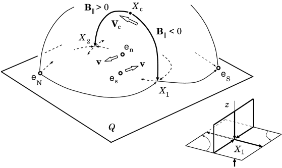
Let us trace how a rapid rearrangement of the field topology occurs under conditions of slow evolution of photospheric sources with the total charge equals zero. We shall arbitrary fix the positions of three charges, while we move the fourth one along an arbitrary trajectory in the plane $Q$.

Let an initial position of the moving charge corresponds to the values of the topological indices $I_{top}=-1$ and + 1 for the zeroth points $X_{1}$ (Type A$-$ with $\lambda_{z}>0$) and $X_{\,2}$ (Type A$+$ with $\lambda_{z}<0$) respectively (Figure 2). Thus two points in the plane $Q$ have different indices. Equation (15) is satisfied. The separator is the field line connecting these points without a coronal null. This field line emerges from the point $X_{1}$ and is directed along the separator to the point $X_{\,2}$. The value and sign of the magnetic-potential difference between the zeroth points are determined from the relation

$$\psi_{\,2}-\psi_{1}=\int\limits_{1}^{2}{\bf B}\,d\,{\bf l}\,,$$ (29)

where the integral is taken along the separator. $\psi_{\,2}-\psi_{1}<0$ for the field shown in Figure 2.

According to Gorbachev et al. [33], the moving charge can arrive in a narrow region (let us call it the region $TT$) such that both points in the plane $Q$ will have the same indices (Figure 11). It follows from the general 3D Equation (15) that in this case there must also exist two zeroth points outside the plane. They are arranged symmetrically relative to the plane $Q$ (the plane $z=0$ in this Section). Figure 12 illustrates how these additional points appear.

Figure 12: Changes of the field pattern at the zeroth point $X_{1}$. (a) An initial state is the non-degenerate point of the Type A$-$ with $\lambda_{z}>0$. (b) A degenerate hyperbolic point (line) with $\lambda_{z}=0$ at the beginning of trigger. (c) After the beginning of trigger, the pattern of field is the non-degenerate point of the Type A$+$ with $\lambda_{z}<0$ and two zeroth points outside the plane $z=0$.

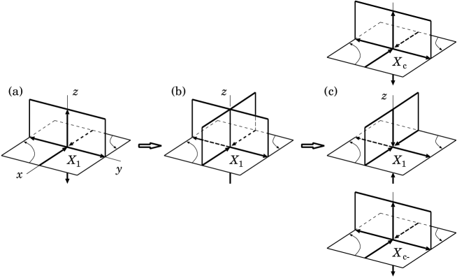
Before the start of trigger, the moving charge is outside of the region $TT$, the index $I_{top}=-1$ and the eigenvalue $\lambda_{z}>0$ at the non-degenerate zeroth point $X_{1}$ (Figure 12a). When the moving charge crosses the boundary of the region $TT$, the eigenvalue $\lambda_{z}$ at the point $X_{1}$ vanishes (Figure 12b):

$$\lambda_{z}(X_{1})=0\,.$$ (30)

The point becomes degenerate. At this instant, another pair of zeroth points is born from the point $X_{1}$ (Figure 12c). We shall consider only one of them, the point $X_{c}$ in the upper half-space $z>0$. This non-degenerate point travels along the separator and merges with the point $X_{\,2}$ in the plane $z=0$ when the moving charge emerges from the region $TT$. At this instant, the eigenvalue $\lambda_{z}$ vanishes:

$$\lambda_{z}(X_{\,2})=0\,.$$ (31)

As a result of the process described, the direction of the field at the separator is reversed with the point $X_{\,2}$ of the Type A$-$ with $\lambda_{z}>0$. After that, the moving charge is located outside the region $TT$, there are no zeroth points outside the plane $z=0$. Thus Equations (30) and (31) determine the boundaries of the topological trigger region $TT$.

Figure 13: The topological trigger (narrow dashed) region is restricted by two boundaries: curves $C_{1}$ and $C_{2}$ corresponding to Equations (30) and (31).

Figure 13 presents an illustrative sample of charge configuration. The fixed charges $e_{1}=-e_{2}=-e_{3}=1$ are located in the plane $Q$ at the points (1; 0), (0; 0) and (0; 1), respectively. The charge $e_{4}=1$ moves along a trajectory shown by a thin curve $Tr$. In the beginning of trigger, it crosses the boundary curve $C_{1}$. Between the boundaries $C_{1}$ and $C_{2}$ there exists a curve $C_{c\,}$ at which $\psi_{2}-\psi_{1}=0$. The field at the separator changes sign at the point $X_{c}\,$. Hence the sections $X_{1}X_{c}$ and $X_{c\,}X_{\,2}$ of the separator make contributions of opposite signs to the integral (29). These contributions exactly compensate each other for a position of the point $X_{c\,}$ when the trajectory $Tr$ crosses the curve $C_{c\,}$.

Typically the region $TT$ is narrow. That is why small shifts of the moving charge within this region lead to large shifts of the zeroth point $X_{c}$ along the separator above the plane $z=0$ just creating a global bifurcation. Using the analogy with hydrodynamics, we see that the separatrix plane ($y,z$) in Figure 12a, which plays the role of a “hard wall” for “flowing in” magnetic flux, is quickly replaced by the orthogonal “hard wall”, the separatrix plane ($x,z$) in Figure 12c. Thus the topological trigger drastically changes directions of magnetic fluxes in an AR as illustrated by Figure 14.

Figure 14: Global changes of the magnetic field configuration related to the topological trigger effect in the model of an active region as illustrated by Figure 13. (a) An initial state before the trigger; the zeroth point $X_{1}$ is the non-degenerate point with a vertical component of magnetic field $B_{z}>0$. (b) After beginning of the trigger, the point $X_{1}$ is the non-degenerate point with $B_{z}<0$; there are two zeroth points outside the plane $z=0$, one of them is shown as $X_{c}$ above the plane $z=0$. (c) The end of the topological trigger process.

Another specific sample is a charge arrangement along a straight line, e.g., the axis $x$ in Figure 1. In this case, owing to the axial symmetry, the entire separator consists of zeroth points. Thus we have a zeroth line. By using an inversion transformation (e.g. Landau et al. [38]):

$${\bf r}^{\prime}=\frac{R^{2}}{r^{2}}\,{\bf r}\,,$$ (32)

where $R$ is the inversion radius, it is easy to show that the axial symmetry is not a necessary condition for the appearance of zeroth line. Moreover, the new zeroth line also represents a circle centered in the plane $z=0$. Thus the 3D zeroth lines of the magnetic field can exist if the sunspots do not lie in a straight line.

Up to now, we have considered the travel of one charge while the coordinates and magnitudes of the other three charges were fixed. It is obvious, however, that all the foregoing remains in force in the more general case of variation of the charge configuration. It follows from the results that a slow evolution of the configuration of field sources in the photosphere can lead to a rapid rearrangement of the global topology in ARs in the corona. The phenomenon of topological trigger is necessary to model the large eruptive flares.

4 Basic physics of reconnection in the corona

4.1 Super-hot turbulent-current layers

Coulomb collisions do not play any role in the super-hot turbulent-current layers (SHTCL). So the plasma inside the SHTCL has to be considered as collisionless (see Somov [19]). The concept of an anomalous resistivity, which originates from wave-particle interactions, is then useful to describe the fast conversion from field energy to particle energy. Some of the general properties of such a collisionless reconnection can be examined in a frame of a self-consistent model which makes it possible to estimate the main parameters of the SHTCL.

Figure 15: A magnetically non-neutral reconnecting layer: the electric current distribution is schematically shown by the shadow, the dotted boundary indicates the field lines going through the current layer. $2a$ is the thickness of the current layer, $2b$ is its width. $2a^{out}$ is an effective cross-section for the outflows of energy and mass along the reconnected magnetic-field lines.

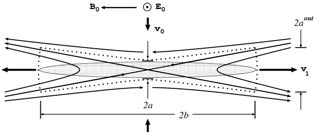
As it reconnects, every magnetic-field line at first penetrates into the current layer with velocity ${\bf v}_{0}$ and later on it moves out with velocity ${\bf v}_{1}$ as illustrated by Figure 15. Basing on the mass, momentum and energy conservation laws, we write the following relations:

$$n_{0}v_{0}\,b=n_{s}v_{1}\,a^{out},$$ (33)

$$2n_{0}k_{{}_{\rm B}}T_{0}+\frac{B_{0}^{\,2}}{8\pi}=n_{s}k_{{}_{\rm B}}T\left(1+\frac{1}{\theta}\right),$$ (34)

$$n_{s}k_{{}_{\rm B}}T\left(1+\frac{1}{\theta}\right)=\frac{1}{2}\,Mn_{s}v_{1}^{\,2}+2n_{0}k_{{}_{\rm B}}T_{0}\,,$$ (35)

$$\chi_{\rm ef}\,{\cal E}_{mag}^{\,in}+{\cal E}_{\,th,e}^{\,in}={\cal E}_{\,th,e}^{\,out}+{\cal C}_{\,\parallel}^{\,an}\,,$$ (36)

$$(1-\chi_{\rm ef})\,{\cal E}_{mag}^{\,in}+{\cal E}_{\,th,i}^{\,in}={\cal E}_{\,th,i}^{\,out}+{\cal K}_{i}^{\,out}\,.$$ (37)

Here $n_{0}$ and $n_{s}$ are the plasma densities outside and inside the layer. $T_{0}$ is the temperature of inflowing plasma outside the layer, $T=T_{e}$ is an effective electron temperature inside it, the ratio $\theta=T_{e}/T_{i}$, $T_{i}$ is an effective temperature of ions. The velocity of electric drift of plasma in direction to the layer

$$v_{0}=V_{d}=c\,\frac{E_{0}}{B_{0}}\,,$$ (38)

and

$$v_{1}=V_{{}_{\rm A,S}}=\frac{B_{0}}{\sqrt{4\pi Mn_{s}}}$$ (39)

is the velocity of the plasma outflow.

The continuity Equation (33) and the energy Equations (36) and (37) are of integral form for a quarter of the layer assumed to be symmetrical and for a unit length along the current. The left-hand sides of (36) and (37) contain the magnetic energy flux

$${\cal E}_{mag}^{\,in}=\frac{B_{0}^{\,2}}{4\pi}\,v_{0}\,b\,,$$ (40)

which creates heating of electrons and ions due to their interactions with waves. A relative fraction $\chi_{\rm ef}$ of the heating is consumed by electrons, while the remaining fraction $(1-\chi_{\rm ef})$ goes to the ions.

The electron and ion temperatures of the plasma inflowing to the layer are the same. Hence, the fluxes of the electron and ion thermal energies are also the same:

$${\cal E}_{\,th,e}^{\,in}={\cal E}_{\,th,i}^{\,in}=\frac{5}{2}\,n_{0}k_{{}_{\rm B}}T_{0}\cdot v_{0}b\,.$$ (41)

The factor 5/2 appears because, for the particles of kind $k$ (electrons, protons, other ions), the mean kinetic energy flux of chaotic motion, $n_{k}m_{k}v_{k}\,w_{k}$, where the heat function per unit mass or, more exactly, the specific enthalpy is

$$w_{k}=\varepsilon_{k}+\frac{p_{k}}{\rho_{k}}=\frac{5}{2}\,\frac{k_{{}_{\rm B}}T_{k}}{m_{k}}\,.$$

Because of the difference between the temperatures of electrons and ions in the outflowing plasma, the electron and ion thermal energy outflows differ:

$${\cal E}_{\,th,e}^{\,out}=\frac{5}{2}\,n_{s}k_{{}_{\rm B}}T\cdot v_{1}a^{out}\,,\quad\,\,{\cal E}_{\,th,i}^{\,out}=\frac{5}{2}\,n_{s}k_{{}_{\rm B}}\frac{T}{\theta}\cdot v_{1}a^{out}\,.$$ (42)

The ion kinetic energy flux from the layer

$${\cal K}_{i}^{\,out}=\frac{1}{2}\,Mn_{s}v_{1}^{\,2}\cdot v_{1}a^{out}$$ (43)

is important in the energy balance (37). As to the electron kinetic energy, it is negligible and disregarded in (36). However, electrons play the dominant role in the heat conductive cooling of a SHTCL:

$${\cal C}_{\,\parallel}^{\,an}=f_{{}_{\rm M}}(\theta)\,\frac{n_{s}(k_{{}_{\rm B}}T)^{3/2}}{M^{1/2}}\,a^{out}.$$ (44)

Here $f_{{}_{\rm M}}(\theta)$ is the function which allows us to consider the field-aligned anomalous thermal flux depending on the the ratio $\theta$.

Under the conditions derived from the Yohkoh and RHESSI data, contributions to the energy balance are not made either by the energy exchange between the electrons and the ions due to collisions, the thermal flux across the magnetic field, and the energy losses for radiation. The field-aligned thermal flux becomes anomalous and plays the dominant role in the cooling of electron component inside the SHTCL. All these properties are typical for collisionless ‘super-hot’ ($T_{e}\stackrel{{\scriptstyle>}}{{{}_{\sim}}}30$ MK) plasma.

Under the same conditions, the anomalous conductivity $\sigma_{\rm ef}$ in the Maxwell equation for ${\rm curl}\,{\bf B}$

$$\frac{cB_{0}}{4\pi a}=\sigma_{\rm ef}E_{0}\,,$$ (45)

as well as the relative fraction $\chi_{\rm ef}$ of the direct heating consumed by electrons, are determined by the wave-particle interaction inside the SHTCL and depend on a type of plasma turbulence and its regime.

4.2 Plasma turbulence inside the SHTCL

In Equation (45) it is convenient to replace the effective conductivity $\sigma_{\rm ef}$ by effective resistivity $\eta_{\,\rm ef}$:

$$\frac{cB_{0}}{4\pi a}=\frac{E_{0}}{\eta_{\,\rm ef}}\,.$$ (46)

In general, the partial contributions to the resistivity may be made simultaneously by several processes of electron scattering by different sorts of waves, so that

$$\eta_{\,\rm ef}=\sum_{k}\eta_{\,k}\,.$$ (47)

The relative share of the electron heating $\chi_{\rm ef}$ is also presented as a sum of the respective shares $\chi_{k}$ of the feasible processes taken, of course, with the weight factors $\eta_{\,k}/\eta_{\,\rm ef}$ which defines the relative contribution from one or another process to the total heating of electrons inside the SHTCL:

$$\chi_{\rm ef}=\sum_{k}\frac{\eta_{\,k}}{\eta_{\,\rm ef}}\,\chi_{k}\,.$$ (48)

In usual practice (e.g. Somov [26]), the sums (47) and (48) consist of no more than two terms, either of which corresponds to one of the turbulent types or states.

4.3 Marginal and saturation regimes

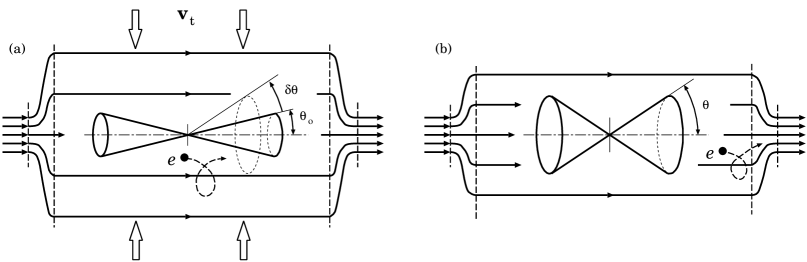
When the electron current velocity $u=j/n_{s}$ exceeds a critical value, the instabilities due to current flow of electrons appear. A rapid decrease in the plasma conductivity occurs and anomalous resistivity arises (Kadomtsev [39], Artsimovich and Sagdeev [40]). The condition needed for current instability in a RCL is that the layer thickness is of the order of the ion gyroradius (Syrovatskii [17]). Thus the turbulent current layers must be sufficiently thin. According to Syrovatskii [41], the development of a thin current layers (TCL) in the solar atmosphere leads to plasma turbulence and correspondingly to a fast rate of field dissipation in flares with the heating of plasma to high temperatures, the high-velocity plasma ejections, and the acceleration of particles to high energies.

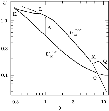
Let us consider the turbulence which is due only to the ion-cyclotron ($ic$) and ion-acoustic ($ia$) instabilities. The sums (47) and (48) consist of no more than two terms; either of which corresponds to one of the said turbulence types. In reality, the ion-cyclotron waves prove to be excited earlier than the ion-acoustic waves at all values of the temperature ratio $\theta\stackrel{{\scriptstyle<}}{{{}_{\sim}}}8$ (Figure 16).

Figure 16: The relative velocity of electrons, $U=u/V_{Te}$ as a function of the ratio $\theta=T_{e}/T_{i}$ inside the SHTCL. The individual ‘arcs’ of the curves correspond to four different regimes of turbulence. The dashed continuations of the ‘arcs’ are the critical velocities of excitation of corresponding waves. The arrow A shows that, in equilibrium plasma with $\theta=1$, the ion-cyclotron waves (the curved section KO) are excited earlier than the ion-acoustic waves (the arc LO).

In the case of the marginal regime of turbulence, the velocity of electrons

$$u=\frac{E_{0}}{en_{s}\,\eta_{\,\rm ef}}$$ (49)

coincides with the critical velocity $u_{k}$ of the $k$-type wave excitation. Hence

$$U_{k}\,(\theta)=U_{k}^{\,mar}\,(\theta)=\frac{u_{k}}{V_{{}_{\rm Te}}}\,\,.$$ (50)

For example, the ion-cyclotron instability becomes enhanced when the velocity $u$ is not lower than the critical value $u_{ic}$ of the ion-cyclotron waves. In the marginal regime

$$U_{ic}^{\,mar}\,(\theta)=\frac{u_{ic}}{V_{{}_{\rm Te}}}\,\,.$$ (51)

This function is shown as the curved section KO in Figure 16.

As long as the ion-cyclotron waves are not saturated, the velocity $u$ remains approximately equal to $u_{\,ic}$ and thus it is possible to calculate the resistivity $\eta_{\,\rm ef}$ from Equation (49). Therefore, if the velocity $u$ in the SHTCL does not exceed the ion-acoustic wave excitation threshold $u_{\,ia}$, only the ion-cyclotron waves will contribute to anomalous resistivity $\eta_{\,\rm ef}$ and the factor $\chi_{\,\rm ef}$.

In the marginal regime, the wave-particle interaction is quasilinear. However, in the case of sufficiently strong electric field $E_{0}$, the nonlinear interactions become important, thereby giving rise to another state of turbulence. In this regime, Ohm’s law can no longer define the resistivity, but determines the the electron current velocity. Regarding the resistivity, this is inferred from the turbulence saturation level. In the saturated regime, $U_{\,k}\,(\theta)$ must be replaced by certain functions $U_{ic}^{\,sat}(\theta)$, shown by the curved section KL in Figure 16, and $U_{ia}^{\,sat}(\theta)$, shown by the arcs MQ for the ion-cyclotron and ion-acoustic turbulence, respectively.

Calculations show that the energy release power and the reconnection rate, which are necessary for solar flares to be accounted for, can be obtained in the marginal regime of ion-acoustic turbulence (see Somov [26,19]).

5 The collapsing magnetic trap effects

5.1 Fast and slow reconnection

Collapsing magnetic traps are formed by the process of collisionless reconnection in the solar atmosphere (Somov and Kosugi [42]). Figure 17 illustrates two possibilities. Fast (Figure 17a) and slow (Figure 17b) modes of reconnection are sketchy shown in the corona above the magnetic obstacle, the region of a strong magnetic field, which is observed in SXRs as a flare loop (shaded).

Figure 17: Plasma flows related to a super-hot turbulent-current layer (SHTCL): the inflows with a relatively low velocity ${\bf v}_{0}$, the downward outflow with a super-Alfvén velocity ${\bf v_{1}}$. (a) SW is the shock wave above the magnetic obstacle.  ${\bf v}_{2}$ is the post-shock velocity, ${\bf v}_{\parallel}$ is the velocity of spreading of the compressed plasma along the field lines toward the feet of the loop. (b) The supra-arcade downflow and collapsing trap without a shock. M₁ and M₂ are the mirroring points where the field becomes sufficiently strong to reflect fast particles above the chromosphere (Ch).

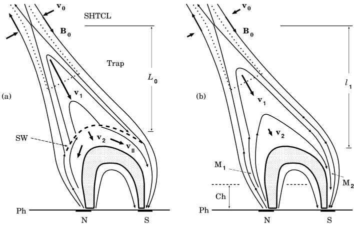
In the first case, let us assume that both feet of a reconnected field loop path through the shock front (SW in Figure 17a) ahead the obstacle. Depending on the velocity and pitch-angle, some of the particles preaccelerated by the SHTCL may penetrate through the magnetic-field jump related to the shock or may be reflected. For the particles reflected by the shock, the magnetic loop represents a trap whose length $L(t)$, the distance between two mirroring points at the shock front, measured along a magnetic-field line, decreases from its initial value $L(0)\approx 2L_{0}$ to zero (the top of the loop goes through the shock front) with the velocity $\approx 2v_{1}$. Therefore, the lifetime of each collapsing trap $t_{1}\approx L_{0}/v_{1}$.

In the case of slow reconnection, there is no a shock wave, and the trap length $L(t)$ is the distance between two mirroring points (M₁ and M₂ in Figure 17b), measured along a reconnected magnetic-field line. In both cases, the electrons and ions are captured in a trap whose length decreases. So the particles gain energy from the increase in parallel momentum.

Thus, in the first approximation, we neglect collisions of particles ahead of the shock wave (Figure 17a) or in the trap without a shock (Figure 17b). In both cases, the particle acceleration can be demonstrated in a simple model – a long trap with short mirrors (Figure 18).

Figure 18: Two main effects in a collapsing trap. (a) Magnetic mirrors move toward each other with velocity ${\bf v}_{m}$. (b) Compression of the trap with velocity ${\bf v}_{t}$.

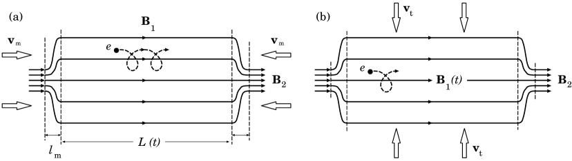
The decreasing length $L(t)$ of the trap is much larger than the length $l_{m}$ of the mirrors; the magnetic field ${\bf B}={\bf B}_{1}$ is uniform inside the trap but grows from ${\bf B}_{1}$ to ${\bf B}_{2}$ in the mirrors. The quantity $B_{2}/B_{1}$ is called the mirror ratio; the larger this ratio, the higher the particle confinement in the trap. The validity conditions for the model are discussed by Somov and Bogachev [43].

5.2 The first-order Fermi-type acceleration

We consider the traps for those the length scale and timescale are both much larger than the gyroradius and gyroperiod of an accelerated particle. Due to strong separation of length and timescales, the magnetic field inside the trap can be considered as uniform and constant (for more detail see Somov and Bogachev [43]). If so, then the longitudinal momentum of a particle increases with a decreasing length $L(t)$, in the adiabatic approximation, as

$$p_{\,\scriptscriptstyle\parallel}(l)=\frac{p_{\,\scriptscriptstyle\parallel\,0}}{l}\,.$$ (52)

Here $l=L(t)/L(0)$ is the dimensionless length of the trap. The transverse momentum is constant inside the trap,

$$p_{\,\scriptscriptstyle\perp}=p_{\,\scriptscriptstyle\perp\,0}\,,$$ (53)

because the first adiabatic invariant is conserved:

$$\frac{p_{\,\scriptscriptstyle\perp}^{\,2}}{B}={\rm const}\,.$$ (54)

Thus the kinetic energy of the particle increases as

$${K}(l)=\frac{p_{\,\scriptscriptstyle\parallel}^{\,2}+p_{\,\scriptscriptstyle\perp}^{\,2}}{2\,m}=\frac{1}{2\,m}\left(\frac{p_{\,\scriptscriptstyle\parallel\,0}^{\,2}}{l^{\,2}}+p_{\,\scriptscriptstyle\perp\,0}^{\,2}\right).$$ (55)

The time of particle escape from the trap, $l=l_{es}$, depends on the initial pitch-angle $\theta_{0}$ of the particle and is determined by the condition

$${\rm tg}\,\theta_{0}=\frac{p_{\,\scriptscriptstyle\perp\,0}}{p_{\,\scriptscriptstyle\parallel\,0}}\,\leq\frac{1}{R\,l_{es}}\,,$$ (56)

where

$$R=\left(\frac{B_{\,2}}{B_{\,1}}-1\right)^{1/2}\,.$$ (57)

The kinetic energy of the particle at the time of its escape is

$${K}_{es}=\frac{p_{\,\scriptscriptstyle\perp\,0}^{\,2}}{2\,m}\,\left(R^{2}+1\right)=\frac{p_{\,\scriptscriptstyle\perp\,0}^{\,2}}{2\,m}\,\frac{B_{\,2}}{B_{\,1}}\,.$$ (58)

One can try to obtain the same canonical result by using more complicated approaches. For example, Giuliani et al. [44] numerically solved the drift equations of motion. However it is worthwhile to explore first the simple analytical approach to investigate the particle energization processes in collapsing traps in more detail before starting to use more sophisticated methods and simulations.

5.3 The betatron acceleration in a collapsing trap

If the thickness of the trap decreases with its decreasing length, then the strength of the field ${\bf B}_{1}$ inside the trap increases as a function of $l$, say $B_{\,1}(l)$. In this case, according to (54), the transverse momentum increases simultaneously with the longitudinal momentum (52):

$$p_{\,\scriptscriptstyle\perp}(l)=p_{\,\scriptscriptstyle\perp\,0}\,\left(\frac{B_{\,1}(l)}{B_{\,1}}\right)^{1/2}\,.$$ (59)

Here $B_{\,1}=B_{\,1}(1)$ is the initial (at $l=1$) value of the field inside the trap. The kinetic energy of a particle

$${K}(l)=\frac{1}{2\,m}\left(\frac{p_{\,\scriptscriptstyle\parallel\,0}^{\,2}}{l^{\,2}}+p_{\,\scriptscriptstyle\perp\,0}^{\,2}\,\frac{B_{\,1}(l)}{B_{\,1}}\right)$$ (60)

increases faster than that in the absence of trap contraction, see (55). Therefore it is natural to assume that the acceleration efficiency in a collapsing trap also increases.

Figure 19: The betatron effect in a collapsing magnetic trap. As the trap is compressed with velocity ${\bf v}_{t}$, the loss cone becomes larger. A particle escapes from the trap earlier with an additional energy due to betatron acceleration.

However, as the trap is compressed, the loss cone becomes larger (Figure 19),

$$\theta_{es}(l)={\rm arcsin}\,\left(\frac{B_{\,1}(l)}{B_{\,2}}\right)^{1/2}\,.$$ (61)

Consequently, the particle escapes from the trap earlier.

On the other hand, the momentum of the particle at the time of its escape satisfies the condition

$${p_{\,\scriptscriptstyle\parallel}}(l)={R}(l)\,{p_{\,\scriptscriptstyle\perp}}(l)\,,$$ (62)

where

$$R(l)=\left(\frac{B_{\,2}}{B_{\,1}(l)}-1\right)^{1/2}\,.$$ (63)

Hence, using (59), we determine the energy of the particle at the time of its escape from the trap

$${K}_{es}=\frac{p_{\,\scriptscriptstyle\perp}(l)^{\,2}}{2\,m}\left(R(l)^{\,2}+1\right)=\frac{p_{\,\scriptscriptstyle\perp\,0}^{\,2}}{2\,m}\,\frac{B_{\,1}(l)}{B_{\,1}}\,\frac{B_{\,2}}{B_{\,1}(l)}\,=\frac{p_{\,\scriptscriptstyle\perp\,0}^{\,2}}{2\,m}\,\frac{B_{\,2}}{B_{\,1}}\,.$$ (64)

The kinetic energy (64), that the particle gains in a collapsing trap with compression, is equal to the energy (58) in a collapsing trap without compression, i.e. without the betatron effect.

Thus the compression of a collapsing trap (as well as its expansion or the transverse oscillations) does not affect the final energy that the particle acquires during its acceleration. The faster gain in energy is exactly offset by the earlier escape of the particle from the trap (Somov and Bogachev [43]). The acceleration efficiency, which is defined as the ratio of the final $(l=l_{ls})$ and initial $(l=1)$ energies, i.e.

$$\frac{{K}_{es}}{{K}(1)}=\frac{p_{\,\scriptscriptstyle\perp\,0}^{\,2}}{p_{\,\scriptscriptstyle\perp\,0}^{\,2}+p_{\,\scriptscriptstyle\parallel\,0}^{\,2}}\,\frac{B_{\,2}}{B_{\,1}}=\left(\frac{p_{\,\scriptscriptstyle\perp\,0}}{p_{\,0}}\right)^{\!2}\,\frac{B_{\,2}}{B_{\,1}}\,,$$ (65)

depends only on the initial mirror ratio $B_{\,2}/B_{\,1}$ and the initial particle momentum or, to be more precise, on the ratio $p_{\,\scriptscriptstyle\perp\,0}/p_{\,0}$. The acceleration efficiency (65) does not depend on the compression of collapsing trap and the pattern of decrease in the trap length either.

It is important that the acceleration time in a collapsing magnetic trap with compression can be much shorter than that in a collapsing trap without compression. For example, if the cross-section area $S(l)$ of the trap decreases proportionally to its length $l$:

$$S(l)=S(1)\,l\,,$$ (66)

then the magnetic field inside the trap

$$B_{\,1}(l)=B_{\,1}(1)\,/\,l\,,$$ (67)

and the effective parameter

$$R(l)=\left(R^{2}-\frac{1-l}{l}\right)^{1/2}\,,$$ (68)

where $R$ is define by formula (57). At the critical length

$$l_{cr}=\frac{1}{1+R^{2}}\,,$$ (69)

the magnetic field inside the trap becomes equal the field in the mirrors, and the magnetic reflection ceases to work. If, for certainty, $B_{\,2}/B_{\,1}=4$, then $l_{cr}=1/4$. So contraction of the collapsing trap does not change the energy of the escaping particles but this energy is reached at an earlier stage of the magnetic collapse when the trap length is finite. In this sense, the betatron effect increases the actual efficiency of the main process – the particle acceleration on the converging magnetic mirrors.

5.4 The betatron acceleration in a shockless trap

If we ignore the betatron effect in a shockless collapsing trap, show in Figure 17b, then the longitudinal momentum of a particle is defined by the formula (instead of (52))

$$p_{\,\parallel}(t)\approx p_{\,\parallel}(0)\,\frac{(l_{1}+l_{2})}{l_{2}+(l_{1}-v_{1}t)}\Rightarrow p_{\,\parallel}(0)\,\frac{(l_{1}+l_{2})}{l_{2}}\,,\quad{\rm when}\quad t\rightarrow t_{1}\,.$$ (70)

The particle acceleration on the magnetic mirrors stops at the time $t_{1}=l_{1}/v_{1}$ at a finite longitudinal momentum that corresponds to a residual length ($l_{2}$ in Figure 17b) of the trap.

Given the betatron acceleration due to compression of the trap, the particle acquires the same energy (58) by this time or earlier if the residual length of the trap is comparable to a critical length $l_{cr}$ determined by a compression law (Somov and Bogachev [43]). Thus the acceleration in shockless collapsing traps with a residual length becomes more plausible. The possible observational manifestations of such traps in the X-ray and optical radiation are discussed by Somov and Bogachev [43]. The most sensitive tool to study behavior of the electron acceleration in the collapsing trap is radio radiation. We assume that wave-particle interactions are important and that two kinds of interactions should be considered in the collapsing trap model.

The first one is resonant scattering of the trapped electrons, including the loss-cone instabilities and related kinetic processes (e.g. Benz [45], Chapter 8). Resonant scattering is most likely to enhance the rate of precipitation of the electrons with energy higher that hundred keV, generating microwave bursts. The lose-cone instabilities of trapped mildly-relativistic electrons (with account taken of the fact that there exist many collapsing field lines at the same time, each line with its proper time-dependent loss cone) would provide excitation of waves with a very wide continuum spectrum. In a flare with a slowly-moving upward coronal HXR source, an ensemble of the collapsing field lines with accelerated electrons would presumably be observed as a slowly moving type IV burst with a very high brightness temperatures and with a possibly significant time delay relative to the chromospheric footpoint emission.

The second kind of wave-particle interactions in the collapsing trap-plus-precipitation model is the streaming instabilities (including the current instabilities related to a return current) associated with the precipitating electrons.

5.5 Some observational results

In order to interpret the temporal and spectral evolution and spatial distribution of HXRs in flares, a two-step acceleration was proposed by Somov and Kosugi [42] with the second step of acceleration via the collapsing magnetic-field lines. The Yohkoh HXT observations of the Bastille-day flare (Masuda et al. [46]) clearly show that, with increasing energy, the HXR emitting region gradually changes from a large diffuse source, which is located presumably above the ridge of soft X-ray arcade, to a two-ribbon structure at the loop footpoints. This result suggests that electrons are in fact accelerated in the large system of the coronal loops, not merely in a particular one. This seems to be consistent with the RHESSI observations of large coronal HXR sources; see, for example, the X4.8 flare of 2002 July 23 (see Figure 3 in Lin et al. [47]).

Efficient trapping and continuous acceleration also produce the large flux and time lags of microwaves that are likely emitted by electrons with higher energies, several hundred keV (Kosugi et al. [48]). The lose-cone instabilities (Benz [45]) of trapped mildly-relativistic electrons in the system of many collapsing field lines (each line with its proper time-dependent lose cone) presumably can provide excitation of radio-wave with a very wide continuum spectrum.

Qiu et al. [49] presented a comprehensive study of the X5.6 flare on 2001 April 6. Evolution of HXRs and microwaves during the gradual phase in this flare exhibits a separation motion between two footpoints, which reflects the progressive reconnection. The gradual HXRs have a harder and hardening spectrum compared with the impulsive component. The gradual component is also a microwave-rich event lagging the HXRs by tens of seconds. The authors propose that the collapsing-trap effect is a viable mechanism that continuously accelerates electrons in a low-density trap before they precipitate into the footpoints.

Imaging radio observations (e.g. Li and Gan [50]) should provide another way to investigate properties of collapsing magnetic traps. It is not simple, however, to understand the observed phenomena relative to the results foreseen by theory. With the incessant progress of magnetic reconnection, the loop system newly formed after reconnection will grow up, while every specific loop will shrink. Just because of such a global growth of flare loops, it is rather difficult to observe the downward motion of newly formed loops. The observations of radio loops by Nobeyama Radioheliograph (NoRH) are not sufficient to resolve specific loops. What is observed is the whole region, i.e., the entire loop or the loop top above it. Anyway, combined microwave and HXR imaging observations are essential in the future.

6 Open issues of reconnection in flares

The existing models of reconnection in the solar corona can be classified in two wide groups: global and local ones (Figure 20).

Figure 20: Models of magnetic reconnection in the solar atmosphere.

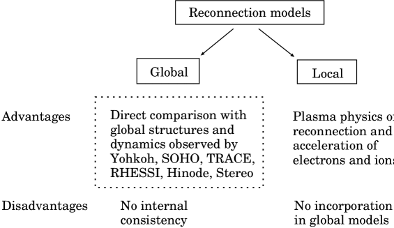
The global models are used to describe actual ARs or even complexes of activity in different approximations and with different accuracies (Somov [51], Gorbachev and Somov [7], Bagalá et al. [52], Antiochos [31], Aschwanden et al. [53], Morita et al. [54], Longcope et al. [55], Barnes [34], Longcope and Beveridge [56], Ugarte-Urra et al. [35]). We make no attempt to review all the models but just remark that the main advantage of the global models is direct comparison between the results of computation and the observed large-scale patterns. For example, the ‘rainbow reconnection’ model (Somov [57]) is used to reproduce the main features of magnetic fields in the corona, related to the large-scale vortex flows in the photosphere.

The advantage of the local models is that they take kinetic effects into account and allow us to develop the basic physics of reconnection in flares. In general, many analytical, numerical, and combined models of reconnection exist in different approximations and with different levels of self-consistency (see Biskamp [15], Priest and Forbes [58]). It becomes more and more obvious that collisionless reconnection in a rarefied plasma is a key process in flares. This process was introduced by Syrovatskii [59] as a dynamic dissipation of field in a current layer and leads to fast conversion from field energy to particle energy, as well as a topological change of the magnetic field (e.g. Horiuchi et al. [60], Yamada et al. [16]).

General properties and parameters of the collisionless reconnection can be examined in a frame of models based on the mass, momentum, and energy conservation laws (Section 4). A particular feature of the models is that electrons and ions are heated by wave-particle interactions in a different way. The magnetic-field-aligned thermal flux becomes anomalous and plays the role in the cooling of electrons in a super-hot turbulent-current layer (SHTCL). These properties seem to be typical for the conditions derived from the observations by Yohkoh and RHESSI (e.g. Joshi et al. [61], Liu et al. [62]), the SOXS mission (Jain et al. [63]). Unfortunately, the local models are not incorporated in the global consideration of reconnection in the corona. Only a few first steps have been made in this direction (see Somov [19]).

Spacecraft observations of collisionless reconnection in the magnetotail and magnetopause as well as recent simulations have shown the existence of thin current layers (TCLs), with scale lengths of the order a few electron skin depth. In the electron MHD model of such TCLs, reconnection is facilitated by electron inertia which breaks the frozen-in condition (Jain and Sharma [64]). The simulations demonstrate the instability of the whistler-like mode which presumably plays the role of the ion-cyclotron instability in the SHTCL model. Stark et al. [65] combine the TCL models with a global model of magnetic field in the magnetosphere.

As for particle acceleration in flares, it goes in two steps. During the first one, the ions and electrons are accelerated by the DC electric field in a super-hot turbulent-current layer (Litvinenko and Somov [66,67]). During the second step, the energy of particles trapped in collapsing traps additionally increases by the first-order Fermi mechanism (Somov and Kosugi [42]) and the betatron mechanism (Somov and Bogachev [43], Karlicky and Kosugi [68]). In a collisionless approximation, Bogachev and Somov [69] show that the collapsing trap model predicts two types of coronal HXR sources: thermal and non-thermal. Thermal sources are formed in traps dominated by the betatron mechanism. Non-thermal sources with power-law spectra appear when electrons are accelerated by the Fermi mechanism. These results are of interest in interpreting the RHESSI observations.

Future models of solar flares should join global and local properties of reconnection under coronal conditions. For example, chains of plasma instabilities, including kinetic instabilities, can be important for our understanding the types and regimes of plasma turbulence inside the collisionless current layers with a longitudinal magnetic field. In particular it is necessary to evaluate better the anomalous resistivity and selective heating of particles in such a SHTCL. Heat conduction is also anomalous in the super-hot plasma. Self-consistent solutions of the reconnection problem will allow us to explain the energy release in flares, including the open question of the mechanism or combination of mechanisms which explains the observed acceleration of electrons and ions to high energy.

To understand the 3D structure of reconnection in flares is one of the most urgent problems. Actual flares are 3D dynamic phenomenon of electromagnetic origin in a highly-conducting plasma with a strong magnetic field. RHESSI and Hinode observations offer us the means to check whether phenomena predicted by topological models (such as the topological trigger) do occur [70]. However some puzzling discrepancies may also exist, and further development of realistic 3D models is required.

References

1 Severny, A.B., Ann. Rev. Astron. Astrophys., 2 (1964), 363.

2 Lin, Y., Wei, X., Zhang, H., Solar Phys., 148 (1993), 133.

3 Wang, J., , Fundamen. Cosmic Phys., 20 (1999), 251.

4 Liu, C., Deng, N., Liu, Y., Falconer, D., Goode, P.R., Denker, C., Wang, H., Astrophys. J., 622 (2005), 722.

5 Wang, H., Liu, C., Deng, Y., Zhang, H., Astrophys. J., 627 (2005), 1031.

6 Sudol, J.J., Harvey, J.W., Astrophys. J., 635 (2005), 647.

7 Gorbachev, V.S., Somov, B.V., Soviet Astronomy–AJ, 33 (1989), 57.

8 Gorbachev, V.S., Somov, B.V., Adv. Space Res., 10 (1990), No. 9, 105.

9 Gorbachev, V.S., Somov, B.V., Solar Phys., 117 (1988), 77.

10 Xiao, C.J., Wang, X.G., Pu, Z.Y., Ma, Z.W., Zhao, H., Zhou, G.P., Wang, J.X., Kivelson, M.G., Fu, S.Y., Liu, Z.X., Zong, Q.G., Dunlop, M.W., Glassmeier, K.-H., Lucek, E., Reme, H., Dandouras, I., Escoubet, C.P., Nature Physics, 3 (2007), 609.

11 Dubrovin, B.A., Novikov, S.P., Fomenko, A.T. Modern Geometry, Nauka (in Russian), Moscow (1986).

12 Syrovatskii, S.I., Soviet Astronomy–AJ, 6 (1962), 768.

13 Brushlinskii, K.V., Zaborov, A.M., Syrovatskii, S.I., Soviet J. Plasma Physics, 6 (1980), 165.

14 Biskamp, D., Phys. Fluids, 29 (1986), 1520.

15 Biskamp, D. Nonlinear Magnetohydrodynamics, Cambridge Univ. Press, Cambridge, UK (1997).

16 Yamada, M., Ren, Y., Ji, H., Gerhardt, S., Dorfman, S., McGeehan, B., AGU, FM, abs. SH43A-03 (2007).

17 Syrovatskii, S.I., Ann. Rev. Astron. Astrophys., 19 (1981), 163.

18 Longcope, D.W., Cowley, S.C., Phys. Plasmas, 3 (1996), 2885.

19 Somov, B.V. Plasma Astrophysics, Part II, Reconnection and Flares, Springer, New York (2006).

20 Cassak, P.A., Drake, J.F., Shay, M.A., Eckhardt, B., Phys. Rev. Lett., 98 (2007), No. 21, id. 215001.

21 Uzdensky, D.A., Phys. Rev. Lett., 99 (2007), No. 26, id. 261101.

22 Greene, J.M., J. Geophys. Res., 93 (1988), 8583.

23 Lau, Y.T., Finn, J.M., Astrophys. J., 350 (1990), 672.

24 Rust, D.M., Somov, B.V., Solar Phys., 93 (1984), 95.

25 Sweet, P.A., Ann. Rev. Astron. Astrophys., 7 (1969), 149.

26 Somov, B.V. Physical Processes in Solar Flares, Kluwer Academic Publ., Dordrecht (1992).

27 Sakai, J.I., de Jager, C., Space Sci. Rev., 77 (1996), 1.

28 Gold, T., Hoyle, F., Monthly Not. Royal Astron. Soc., 120 (1960), 89.

29 Pevtsov, A.A., Canfield, R.C., Zirin, H., Astrophys. J., 473 (1996), 533.

30 Den, O.G., Somov, B.V., Soviet Astronomy–AJ, 33 (1989), 149.

31 Antiochos, S.K., Astrophys. J., 502 (1998), L181.

32 Parnell, C.E., Solar Phys., 242 (2007), 21.

33 Gorbachev, V.S., Kel’ner, S.R., Somov, B.V., Shwarz, A.S., Soviet Astronomy–AJ, 32 (1988), 308.

34 Barnes, G., Astrophys. J., 670 (2007), L53.

35 Ugarte-Urra, I., Warren, H.P., Winebarger, A.R., Astrophys. J., 662 (2007), 1293.

36 Syrovatskii, S.I., Somov, B.V. in M. Dryer and E. Tandberg-Hanssen (eds.), Solar and Interplanetary Dynamics, IAU Symp. 91, Reidel, Dordrecht (1980), pp. 425-441.

37 Syrovatskii, S.I., Solar Phys., 76 (1982), 3.

38 Landau, L.D., Lifshitz, E.M., Pitaevskii, L.P. Electrodynamics of Continuous Media, Pergamon Press, Oxford (1984).

39 Kadomtsev, B.B. Collective Phenomena in Plasma, Nauka (in Russian), Moscow (1976).

40 Artsimovich, L.A., Sagdeev, R.Z. Plasma Physics for Physicists, Atomizdat, Moscow (1979).

41 Syrovatskii, S.I. in E.R. Dyer (ed.), Solar-Terrestrial Physics 1970, Part 1, D. Reidel Publ., Dordrecht, Holland (1972), pp. 119-133.

42 Somov, B.V., Kosugi, T., Astrophys. J., 485 (1997), 859.

43 Somov, B.V., Bogachev, S.A., Astronomy Lett., 29 (2003), 621.

44 Giuliani, P., Neukirch, T., Wood, P., Astrophys. J., 635 (2005), 636.

45 Benz, A. Plasma Astrophysics: Kinetic Processes in Solar and Stellar Coronae, Kluwer Academic Publ., Dordrecht (2002).

46 Masuda, S., Kosugi, T., Hudson, H.S., Solar Phys., 204 (2001), 57.

47 Lin, R.P., Krucker, S., Hurford, G.J., Smith, D.M., Hudson, H.S., Holman, G.D., Schwartz, R.A., Dennis, B.R., Share, G.H., Murphy, R.J., Emslie, A.G., Johns-Krull, C., Vilmer, N., Astrophys. J., 595 (2003), L69.

48 Kosugi, T., Dennis, B.R., Kai, K., Astrophys. J., 324 (1988), 1118.

49 Qiu, J., Lee, J., Gary, D.E., Astrophys. J., 603 (2004), 335.

50 Li, Y.P., Gan, W.Q., Astrophys. J., 629 (2005), L137.

51 Somov, B.V., Soviet Phys. Usp., 28 (1985), 271.

52 Bagalá, L.G., Mandrini, C.H., Rovira, M.G., Démoulin, P., Hénoux, J.C., Solar Phys., 161 (1995), 103.

53 Aschwanden, M.J., Kosugi, T., Hanaoka, Y., Nishio, M., Melrose, D., Astrophys. J., 526 (1999), 1026.

54 Morita, S., Uchida, Y., Hirose, S., Uemura, S., Yamaguchi, T., Solar Phys., 200 (2001), 137.

55 Longcope, D.W., McKenzie, D.E., Cirtain, J., Scott, J., Astrophys. J., 630 (2005), 596.

56 Longcope, D.W., Beveridge, C., Astrophys. J., 669 (2007), 621.

57 Somov, B.V., Astron. Astrophys., 163 (1986), 210.

58 Priest, E.R. and Forbes, T. Magnetic Reconnection: MHD Theory and Applications, Cambridge Univ. Press, Cambridge, UK (2000).

59 Syrovatskii, S.I., Soviet Physics–JETP, 23 (1966), 754.

60 Horiuchi, R., Pei, W., Sato, T., Earth Planets Space, 53 (2001), 439.

61 Joshi, B., Manoharan, P.K., Veronig, A.M., Pant, P., Pandey, K., Solar Phys., 242 (2007), 143.

62 Liu, W., Petrosian, V., Dennis, B.R., Jiang, Y.W., Astrophys. J., 676 (2008), 704.

63 Jain, R., Pradhan, A.K., Joshi, V., Shah, K.J., Trivedi, J.J., Kayasth, S.L., Shah, V.M., Deshpande, M.R., Solar Phys., 239 (2006), 217.

64 Jain, N., Sharma, A.S., AGU, FM, abs. SM31D-0659 (2007).

65 Stark, D., Sharma, A., Jain, N., AGU, FM, abs. SM31C-1465 (2007).

66 Litvinenko, Y.E., Somov, B.V., Solar Phys., 146 (1993), 127.

67 Litvinenko, Y.E.; Somov, B.V., Solar Phys., 158 (1995), 317.

68 Karlický, M., Kosugi, T., Astron. Astrophys., 419 (2004), 1159.

69 Bogachev, S.A., Somov, B.V., Astronomy Letters, 33 (2007), 54.

70 Somov, B.V., Astronomy Letters, 34 (2008), 635.