Geometry of the Central Limit Theorem in the Nonextensive Case

Abstract

We uncover geometric aspects that underlie the sum of two independent stochastic variables when both are governed by $q-$Gaussian probability distributions. The pertinent discussion is given in terms of random vectors uniformly distributed on a $p-$sphere.

1 Introduction

Nonextensive statistical physics provides a rich framework for the interpretation of complex systems’ behavior whenever classical statistical physics fails [1]. The basic tool for this approach is the extension of the classical Boltzmann entropy to the wider class of Tsallis entropies. In this context, the usual Gaussian distributions is extended to the q-Gaussian distributions, to be defined below. The study of the properties of these distributions is an interesting problem, being the subject of a number of recent publications [1]. Of special interest is the extension of the usual stability result that holds in the Gaussian case, namely, that if $X_{1}\in\mathbb{R}$ and $X_{2}\in\mathbb{R}$ are independent Gaussian random variables with unit variance, then the linear combination

$$Z=a_{1}X_{1}+a_{2}X_{2}$$

is again Gaussian and

$$Z\sim\sqrt{a_{1}^{2}+a_{2}^{2}}X,$$ (1)

where $X$ is Gaussian with unit variance, and $\sim$ denotes equality in distribution.

This stability property is at the core of the central limit theorem (CLT), which describes the behavior of systems that result of the additive superposition of many independent phenomena. The CLT can be ranked among the most important results in probability theory and statistics, and plays an essential role in several disciplines, notably in statistical mechanics. Pioneers like A. de Moivre, P.S. de Laplace, S.D. Poisson, and C.F. Gauss have shown that the Gaussian distribution is the attractor of the superposition process of independent systems with a finite second moment. Distinguished authors like Chebyshev, Markov, Liapounov, Feller, Lindeberg, and Lévy have also made essential contributions to the CLT-development. As far as physics is concerned one can state that, starting from any system with any finite variance distribution function (for some measurable quantity $x$), and combining additively a sufficiently large number of such independent systems together, the resultant distribution function of $x$ is always Gaussian.

A natural question is thus the extension of the stability result (1) to the nonextensive case, that is, for q-Gaussian distributions. This interesting problem is currently the subject of several publications (see for example [2]) in which possible extensions of the CLT to the nonextensive context are studied. The aim of this communication is to give some geometric insight into the behavior of q-Gaussian distributions for the case $q<1$.

2 Definitions and notations

In nonextensive statistics, the usual Shannon entropy of a density probability $f_{X}$, namely

$$H_{1}\left(X\right)=-\int f_{X}\log f_{X}$$

is replaced by its Tsallis version

$$H_{q}\left(X\right)=\frac{1}{1-q}\left(1-\int f_{X}^{q}\right)$$

where the nonextensivity index $q$ is a real parameter, usually taken to be positive. It can be checked by applying L’Hospital’s rule that Shannon’s entropy coincides with the limit case

$$\lim_{q\to 1}H_{q}\left(X\right)=H_{1}\left(X\right)$$

It is a well-known result that the distribution that maximizes the Shannon entropy under a covariance matrix constraint $EXX^{T}=K$ (where $K$ is a symmetric definite positive matrix) is the Gaussian distribution

$$f_{X}\left(X\right)=\frac{1}{|\pi K|^{\frac{1}{2}}}\exp\left(-X^{T}K^{-1}X\right).$$

Its nonextensive counterpart, called a q-Gaussian, is defined as follows.

Definition 1

The $n-$variate distribution with zero mean and given covariance matrix $EXX^{T}=K$ having maximum Tsallis entropy is denoted as $G_{q}\left(K\right)$ and defined as follows for $0<q<1:$

$$f_{X}\left(X\right)=A_{q}\left(1-X^{t}\Sigma^{-1}X\right)_{+}^{\frac{1}{1-q}},$$ (2)

with matrix $\Sigma=pK$, parameter $p$ defined as $p=2\frac{2-q}{1-q}+n$ and notation $\left(x\right)_{+}=\max\left(x,0\right).$ Moreover, the partition function is

$$A_{q}=\frac{\Gamma\left(\frac{2-q}{q-1}+\frac{n}{2}\right)}{\Gamma\left(\frac{2-q}{1-q}\right)|\pi\Sigma|^{1/2}}.$$

We note that this distribution has bounded support; namely, $f_{X}\left(X\right)\neq 0$ only when $X$ belongs the ellipsoïd

$$\mathcal{E}_{\Sigma}=\left\{Z\in\mathbb{R}^{n}\,;\,Z^{t}\Sigma^{-1}Z\leq 1\right\}.$$

We also need the notion of spherical vector, defined as follows:

Definition 2

A random vector $X\in\mathbb{R}^{n}$ is spherical if its density $f_{X}$ is a function of the norm $|X|$ of $X$ only, namely

$$f_{X}\left(X\right)=g\left(|X|\right)$$

for some function $g:\mathbb{R}^{+}\to\mathbb{R}^{+}.$

An alternative characterization of a spherical vector is as follows [3]:

Proposition 3

A random vector $X\in\mathbb{R}^{n}$ is spherical if

$$X\sim AX$$

for any orthogonal matrix $A,$ where sign $\sim$ denotes equality in distribution.

This property highlights the importance of spherical vectors in physics since they describe systems that are invariant by orthogonal transformation.

A fundamental property of a spherical vector is the following:

Proposition 4

[3] If $X\in\mathbb{R}^{n}$ is a spherical random vector, then it has the stochastic representation

$$X\sim rU$$

where $U$ is a uniform vector on the sphere $\mathcal{S}_{n}=\left\{X\in\mathbb{R}^{n};\,X^{T}X=1\right\}$ and $r$ is a positive scalar random variable independent of $U.$ Moreover, $r$ has stochastic representation

$$r\sim|X|.$$ (3)

3 A heuristic approach

We start with a heuristic approach to the stability problem, namely the behavior of the random variable $Z=a_{1}X_{1}+a_{2}X_{2}$ when $X_{1}$ and $X_{2}$ are two unit variance, q-Gaussian independent random vectors in $\mathbb{R}^{n}$ with nonextensivity parameter $q<1;$ let us assume that the following hypothesis - called (H) hypothesis :

$$n+\frac{2}{1-q}\in\mathbb{N},$$ (4)

holds so that $\frac{1}{1-q}=\frac{p-n}{2}-1$ where $p>n$ is an integer; a classical result is that $X_{1}$ (resp. $X_{2}$) can then be considered as the $n-$dimensional marginal vector of a random vector $U_{1}$ (resp. $U_{2}$) that is uniformly distributed on the unit sphere $\mathcal{S}_{p-1}$ in $\mathbb{R}^{p}.$ Thus, there exist random vectors $\tilde{X}_{1}$ and $\tilde{X}_{2}$ in $\mathbb{R}^{p-n}$ such that

$$U_{1}=\left[\begin{array}[]{c}X_{1}\\ \tilde{X}_{1}\end{array}\right]\,\,\text{and}\,\,U_{2}=\left[\begin{array}[]{c}X_{2}\\ \tilde{X}_{2}\end{array}\right]$$

are two $p-$dimensional independent vectors uniformly distributed on $\mathcal{S}_{p}.$ Then, the sum $U_{1}+U_{2}$ is a spherical vector and has stochastic representation

$$a_{1}U_{1}+a_{2}U_{2}\sim rU$$

where $U$ is uniform on $\mathcal{S}_{p}.$ Now, by equation (3), the random variable $r$ is distributed as

$$r\sim|a_{1}U_{1}+a_{2}U_{2}|=\sqrt{a_{1}^{2}+a_{2}^{2}+2\lambda a_{1}a_{2}}$$

where $\lambda=U_{1}^{T}U_{2}:$ this can be easily deduced from

$$|a_{1}U_{1}+a_{2}U_{2}|=\sqrt{a_{1}^{2}U_{1}^{T}U_{1}+a_{2}^{2}U_{2}^{T}U_{2}+2a_{1}a_{2}U_{1}^{T}U_{2}}$$

remarking that $U_{1}^{T}U_{1}=U_{2}^{T}U_{2}=1.$ But $\lambda$ is a random variable with q-Gaussian distribution! We prove this result by noticing that, conditioned to $U_{2}=u_{2},$ random variable $\lambda$ is the angle between $U_{1}$ and the fixed direction $u_{2}.$ Since $U_{1}$ is spherical, we may restrict our attention to the angle between $U_{1}$ and the first vector of the canonical basis in $\mathbb{R}^{n},$ so that we look for the distribution of the first component of $U_{1}$, which follows a q-Gaussian distribution with parameter $q_{\lambda}$ such that

$$\frac{1}{1-q_{\lambda}}=\frac{p-1}{2}-1.$$

Since this distribution does not depend on our initial choice $U_{2}=u_{2},$ random variable $\lambda$ follows unconditionally the above cited distribution. We conclude that the $n-$dimensional marginal $Z=a_{1}X_{1}+a_{2}X_{2}$ of vector $a_{1}U_{1}+a_{2}U_{2}$ is distributed as

$$a_{1}X_{1}+a_{2}X_{2}\sim rX$$

where $X$ is the $n-$dimensional marginal vector of $U$ so that $X$ is again $q-$Gaussian with parameter $q.$ Moreover, this result extends to the case where $X_{1}$ and $X_{2}$ both have a covariance matrix $K\neq I$ by multiplying vectors $X_{1}$ and $X_{2}$ by matrix $K^{\frac{1}{2}}.$ Consequently, we have deduced the following

Theorem 5

If $X_{1}$ and $X_{2}$ are two q-Gaussian independent random vectors in $\mathbb{R}^{n}$ with covariance matrix $K$ and nonextensivity parameter $q<1$ and if hypothesis (H) holds then

$$a_{1}X_{1}+a_{2}X_{2}\sim\left(a_{1}\circ a_{2}\right)X$$

where $X$ is again q-Gaussian with same covariance matrix $K$ and same nonextensive parameter $q$ as $X_{1}$, and where

$$a_{1}\circ a_{2}=\sqrt{a_{1}^{2}+a_{2}^{2}+2\lambda a_{1}a_{2}},$$ (5)

the random variable $\lambda$ being independent of $X$ and again q-Gaussian distributed with nonextensive parameter $q_{\lambda}$ defined by

$$q_{\lambda}=\frac{\left(n-1\right)-\left(n-3\right)q}{\left(n+1\right)-\left(n-1\right)q}.$$ (6)

Two remarks are of interest at this point:

• the univariate framework $n=1$ is the only case for which random variable $\lambda$ has the same nonextensivity parameter $q_{\lambda}$ as $X_{1}$ and $X_{2}$;

• however, we note that

  $$\lim_{n\to+\infty}q_{\lambda}=1.$$

  This means that for large dimensional systems, the random variable $\lambda$ converges to the constant $0$ and we recover the deterministic convolution; this is coherent with the fact that large dimensional $q-$Gaussian vectors are ”close” to Gaussian vectors by De-Finetti inequality.

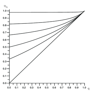
The curves in Figure 1 show the nonextensive parameter $q_{\lambda}$ as a function of $q$ for several values of dimension $n.$

Figure 1: nonextensivity parameter $q_{\lambda}$ as a function of $q$ for dimensions $n=1,2,3,5,10$ and $100$ (bottom to top)

More can be said about the algebra $a_{1}\circ a_{2}$:

Theorem 6

The algebra $a_{1}\circ a_{2}$ defined as in (5) is associative and for any $n\geq 2,$

$$a_{1}\circ a_{2}\circ...\circ a_{n}=\sqrt{\sum_{i=1}^{n}a_{i}^{2}+2\sum_{i<j}\lambda_{ij}a_{i}a_{j}}$$

where random variables $\lambda_{ij}=U_{i}^{T}U_{j}$ are q-Gaussian.

As an example,

$$a_{1}\circ a_{2}\circ a_{3}=\sqrt{a_{1}^{2}+a_{2}^{2}+a_{3}^{2}+2\lambda_{12}a_{1}a_{2}+2\lambda_{13}a_{1}a_{3}+2\lambda_{23}a_{2}a_{3}}.$$

[Proof] By definition,

$$a_{1}\circ a_{2}\circ...\circ a_{n} = |\sum_{i=1}^{n}a_{i}U_{i}|$$

$$= \sqrt{\sum_{i=1}^{n}a_{i}^{2}U_{i}^{t}U_{i}+2\sum_{i<j}a_{i}a_{j}U_{i}^{t}U_{j}}$$

Since $|U_{i}|=1$, we deduce, by denoting $U_{i}^{t}U_{j}=\lambda_{ij}$, that

$$a_{1}\circ a_{2}\circ...\circ a_{n}=\sqrt{\sum_{i=1}^{n}a_{i}^{2}+2\sum_{i<j}\lambda_{ij}a_{i}a_{j}}.$$

By the same proof as above, we deduce that each $\lambda_{i}$ is $q-$Gaussian distributed with parameter $q_{\lambda}.$ We remark that random variables $\lambda_{i,j}$ are independent pairwise but are obviously not mutually independent.

4 Generalization

The preceding result was derived under the hypothesis (H) as expressed by (4), that is, for specific values of $q<1$ only; we show in this section that this result holds in fact without this hypothesis - for all values of $q<1$ - but the proof requires more elaborate analytic tools. Our main result is

Theorem 7

Theorem 5 holds for all values of $q$ such that $0<q<1.$

[Proof] The characteristic function associated to the $q-$Gaussian distribution (2) is

$$\varphi_{X}(u)\overset{d}{=}E\exp\left(iu^{T}X\right)=2^{\frac{p}{2}-1}\Gamma\left(\frac{p}{2}\right)\frac{J_{\frac{p}{2}-1}\left(\sqrt{u^{T}Ku}\right)}{\left(\sqrt{u^{T}Ku}\right)^{\frac{p}{2}-1}}$$

where $J_{\frac{p}{2}-1}$ is the Bessel function of the first kind and with parameter $\frac{p}{2}-1$ where

$$p=2\frac{2-q}{1-q}+n.$$

According to Gegenbauer [4, 367, eq.16],

$$2^{\nu}\Gamma\left(\nu+\frac{1}{2}\right)\Gamma\left(\frac{1}{2}\right)\frac{J_{\nu}\left(Z\right)}{Z^{\nu}}\frac{J_{\nu}\left(z\right)}{z^{\nu}}=\int_{0}^{\pi}\frac{J_{\nu}\left(\sqrt{Z^{2}+z^{2}-2Zz\cos\phi}\right)}{\left(Z^{2}+z^{2}-2Zz\cos\phi\right)^{\frac{\nu}{2}}}\sin^{2\nu}\phi d\phi.$$

Choosing $Z=a_{1}\sqrt{u^{T}Ku}$, $z=a_{2}\sqrt{u^{T}Ku},$ $\lambda=-\cos\phi$ and $\nu=\frac{p}{2}-1,$ this equality can be rewritten as

$$\varphi_{a_{1}X_{1}}\left(u\right)\varphi_{a_{2}X_{2}}\left(u\right)=\varphi_{\sqrt{a_{1}^{2}+a_{2}^{2}+2\lambda a_{1}a_{2}}X}\left(u\right)$$

where $\lambda$ is distributed according to

$$f\left(\lambda\right)=\frac{\Gamma\left(\nu+1\right)}{\Gamma\left(\nu+\frac{1}{2}\right)\Gamma\left(\frac{1}{2}\right)}\left(1-\lambda^{2}\right)^{\nu-\frac{1}{2}}.$$

Since $q_{\lambda}$ is defined by

$$\frac{1}{1-q_{\lambda}}=\nu-\frac{1}{2}=\frac{p-1}{2}-1,$$

we deduce (6). Let us recall the scaling behavior of Gaussian vectors

$$a_{1}X_{1}+a_{2}X_{2}\sim\sqrt{a_{1}^{2}+a_{2}^{2}}X$$

which can be probabilistically interpreted in the context of $\alpha-$stable distributions: a distribution $f_{\alpha}$ is $\alpha-$stable if, for $X_{1}$ and $X_{2}$ independent with distribution $f_{\alpha}$, the linear combination

$$a_{1}X_{1}+a_{2}X_{2}\sim\left(|a_{1}|^{\alpha}+|a_{2}|^{\alpha}\right)^{\frac{1}{\alpha}}X,$$

where $X$ follows again distribution $f_{\alpha}.$ Thus, a Gaussian distribution is $\alpha-$stable with $\alpha=2.$ The result of Thm.1 can be viewed as follows: $q-$Gaussians are not $\alpha-$stable (unless $q=1$ which corresponds to the Gaussian case $\alpha=2$); however, their scaling behavior is close to the Gaussian $\alpha=2$ case, except for the fact that the scaling variable $a_{1}\circ a_{2}$ includes an additional random term $\lambda$.

5 Geometric interpretation

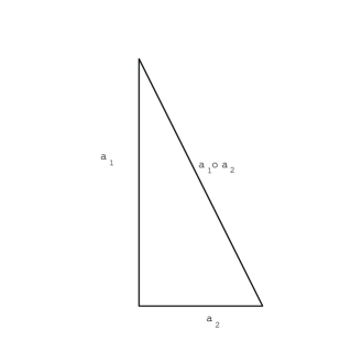
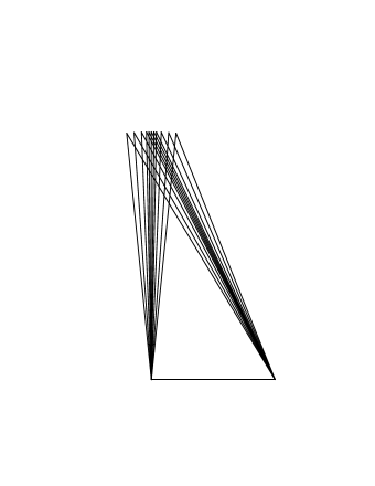
Geometrically, the Gaussian scaling factor $\sqrt{a_{1}^{2}+a_{2}^{2}}$ can be interpreted, according to Pythagoras’ theorem, as the length of the hypotenuse of a right triangle with sides of lengths $|a_{1}|$ and $|a_{2}|$. The $q-$Gaussian case corresponds to a triangle for which the angle between $|a_{1}|$ and $|a_{2}|$, let us call it $\phi$, fluctuates around rectangularity.

Figure 2: the geometric interpretation of $a_{1}\circ a_{2}$ in the Gaussian case ($q=1$ left); in the $q-$Gaussian case (left), $a_{1}\circ a_{2}$ is randomly chosen as one of the hypothenuses represented, the angle $\phi$ between sides $a_{1}$ and $a_{2}$ being distributed as shown on Figure 3

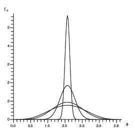
The distribution of the angle $\phi$ where $\lambda=-\cos\phi$ is given by

$$f_{\phi}\left(\phi\right)=\frac{\Gamma\left(\nu+1\right)}{\Gamma\left(\nu+\frac{1}{2}\right)\Gamma\left(\frac{1}{2}\right)}\sin^{2\nu}\phi,\,\,0\leq\phi\leq\pi,\,\,\nu=\frac{1}{1-q_{\lambda}}+\frac{1}{2}.$$

This distributions is shown in Figure 3 for values of the parameter $q=0.99,\,0.9,\,0.5$ and $0.1$ (top to bottom).

Figure 3: the distribution of angle $\phi$ for values of the parameter $q_{\lambda}=0.99,\,0.9,\,0.5$ and $0.1$ (top to bottom).

We remark that this distribution is symmetric around the angle $\phi=\frac{\pi}{2}$ and that, as $q\to 1,$ the angle $\phi$ becomes deterministic and equal to $\frac{\pi}{2}$. Further, the usual scaling law for Gaussian distributions (1) is recovered.

5.1 An optical analogy

We remark that formula (5) exhibits a close resemblance with the interference formula for the amplitude of the superposition of two optical beams. Interferometric optical testing is based on these phenomena of interference. Two-beam interference is the superposition of two waves, such as the disturbance of the surface of a pond by a small rock encountering a similar pattern from a second rock. When two wave crests reach the same point simultaneously, the wave height is the sum of the two individual waves. Conversely, a wave trough and a wave crest reaching a point simultaneously will cancel each other out. Water, sound, and light waves all exhibit interference. A light wave can be described by its frequency, amplitude, and phase, and the resulting interference pattern between two waves depends on these properties, among others. Our present interest lies in the two-beam interference equation. It gives the irradiance $I$ [6] for monochromatic waves of irradiance $I_{1},$ and $I_{2}$ in terms of the phase difference $\Delta_{1,\,2}$ expressed as $\cos{\phi}=\cos{(\phi_{1}-\phi_{2})}$. We have

$$I=I_{1}+I_{2}+2\sqrt{I_{1}I_{2}}\cos{\phi},$$

and, in terms of the $A-$amplitudes $I=A^{2}$,

$$A^{2}=A_{1}^{2}+A_{2}^{2}+2A_{1}A_{2}\cos{\phi}.$$

If the emission of the two beams could be so arranged that the phase difference becomes random [7, 8, 9], this physical analogy would be exact.

5.2 Study of the composition law $\circ$

The composition law

$$a_{1}\circ a_{2}=\sqrt{a_{1}^{2}+a_{2}^{2}+2\lambda a_{1}a_{2}}$$

has been studied in [5], in the more general case where $a_{1}$ and $a_{2}$ are independent, positive random variables. The associativity result is as follows

Theorem 8

[5, p.18 thm.1] The composition law $\circ$ is associative if and only if either

$$a_{1}\circ a_{2}=\sqrt{a_{1}^{2}+a_{2}^{2}}$$

or

$$a_{1}\circ a_{2}=|a_{1}|+|a_{2}|$$

or

$$a_{1}\circ a_{2}=\sqrt{a_{1}^{2}+a_{2}^{2}+2\lambda a_{1}a_{2}}$$ (7)

where $\lambda\sim G_{q}\left(0,1\right)$ for some $q\geq 0.$

This theorem can be interpreted as follows: the only cases where the composition law $\circ$ is associative is

1. the Gaussian case ($q=1,\,q_{\lambda}=1$)

2. the Cauchy case ($q=2$)

3. the present $q-$Gaussian case with $0\leq q<1$

It is thus a remarkable property that the only cases of associativity of this composition law correspond to the whole range of $q-$Gaussian distributions with $0\leq q\leq 1$ or to the Cauchy case $q=2$. We note moreover that in the limit case $q=0,$ $a_{1}\circ a_{2}$ in (7) reduces to a Bernoulli random variable that takes values $a_{1}+a_{2}$ and $a_{1}-a_{2}$ with probability $\frac{1}{2}.$

5.3 A Central Limit Theorem for the composition law $\circ$

In the same spirit as the central limit theorem for the usual addition, a central limit theorem exists for the composition law $\circ$. Before we give its rigourous expression as established in [5], let us look at a special case of it based on the theory of superstatistics. Let us consider the random walk

$$S_{n}=\frac{1}{\sigma\sqrt{n}}\sum_{i=1}^{n}X_{i}$$

where $X_{i}$ are independent $q-$Gaussian random variables with same variance $\sigma^{2}$ and where $q<1;$ since all $X_{i}$ have finite variance, the usual Central Limit theorem applies and

$$S_{n}\to\mathcal{N}\left(0,1\right).$$

But by theorems (6) and (7), we have also

$$S_{n}=\left(\bigotimes_{i=1}^{n}\frac{1}{\sigma\sqrt{n}}\right)X$$

with notation

$$\bigotimes_{i=1}^{n}a_{i}=a_{1}\circ\dots\circ a_{n}$$

where $X$ is $q-$Gaussian with the same nonextensivity parameter $q.$ Since, by the superstatistics theory, a Gaussian random variable $G$ can be decomposed as

$$G=\chi_{p}X$$

where $\chi_{p}$ is chi-distributed with $p$ degrees of freedom, we deduce that the following limit

$$\bigotimes_{i=1}^{n}\frac{1}{\sigma\sqrt{n}}=\frac{1}{\sigma\sqrt{n}}\bigotimes_{i=1}^{n}\,1\underset{n\to+\infty}{\longrightarrow}\chi_{p}$$

should hold. But this result is easy to check at least under hypothesis (H): in this case,

$$S_{n}=r_{n}X$$

where

$$r_{n}=|\sum_{i=1}^{n}U_{i}|$$

where $U_{i}$ are independent and uniformly distributed on the sphere $\mathcal{S}_{p-1}.$ By the Central Limit Theorem, $r_{n}\to|G|$ where $G$ is a Gaussian vector in $\mathbb{R}^{p}$; hence $r_{n}$ converges indeed to a $\chi$ distributed random variable with $p$ degrees of freedom.

It turns out that a much more general result holds, namely

Theorem 9

[5] If $\left\{a_{i}\right\}$ are positive, independent and identically distributed random variables with variance $\sigma$, then the composition

$$\frac{1}{\sigma\sqrt{n}}\bigotimes_{i=1}^{n}a_{i}\underset{n\to+\infty}{\longrightarrow}\chi_{p}$$

where $\chi_{p}$ is a chi-distributed random variablewith parameter $p.$

This result can be considered as a central limit theorem for the algebra $\circ$ defined by (5).

6 Conclusions

In this work we have uncovered interesting geometric aspects that underlie the sum $Z$ of two stochastic variables $a_{1}X$ and $a_{2}X_{2}$ ($a_{1}$, $a_{2}$ are scalars and $X_{1}$, $X_{2}$ are $n-$variate vectors). The alluded geometry becomes operative when the two variables are governed by $q-$Gaussian probability distributions with $q<1$. We found that its sum $Z$ turns out to be $q-$Gaussian with same nonextensivity parameter $q$ multiplied by an independent random factor $a_{1}\circ a_{2}$. In turn, the random factor can be described as a random and symmetric mixture of the two constants $a_{1}$ and $a_{2}$, the random factor involved following itself a $q-$Gaussian distribution.

References

• [1] C. Tsallis, Introduction to Nonextensive Statistical Mechanics: Approaching a Complex World (Springer-Verlag, New York, 2009)
• [2] S. Umarov, C. Tsallis, S. Steinberg, On a q-Central Limit Theorem Consistent with Nonextensive Statistical Mechanics, Milan Journal of Mathematics, 76-1, 307-328, 2008
• [3] K.-T. Fang , S. Kotz, K. W. Ng, Symmetric Multivariate and Related Distributions, Chapman & Hall/CRC, 1989
• [4] G.N. Watson, A treatise on the theory of Bessel functions, second edition, Cambridge, (1944)
• [5] J.F.C. Kingman, Random walks with spherical symmetry, Acta Math. 109, 11-53, (1965).
• [6] Irradiance, radiant emittance, and radiant exitance are radiometry terms for the power of electromagnetic radiation at a surface, per unit area. The term irradiance is used when the electromagnetic radiation is incident on the surface.
• [7] T. Setala, A. Shevchenko, M. Kaivola, and A. T. Friberg, Phys. Rev. A 78, 033817 (2008).
• [8] V. P. Lukin, Kvantovaia Elektronika (Moscow), 7, 1270 (1980).
• [9] Z. H. Gu, H. M. Escamilla, E. R. Mendez, A. A. Maradudin, J. Q. Lu, T. Michel, M. Nieto-Vesperinas, Applied Optics 31, 5878 (1992).