A curvature theory for discrete surfaces
based on mesh parallelity

Abstract.

We consider a general theory of curvatures of discrete surfaces equipped with edgewise parallel Gauss images, and where mean and Gaussian curvatures of faces are derived from the faces’ areas and mixed areas. Remarkably these notions are capable of unifying notable previously defined classes of surfaces, such as discrete isothermic minimal surfaces and surfaces of constant mean curvature. We discuss various types of natural Gauss images, the existence of principal curvatures, constant curvature surfaces, Christoffel duality, Koenigs nets, contact element nets, s-isothermic nets, and interesting special cases such as discrete Delaunay surfaces derived from elliptic billiards.

1. Introduction

A new field of discrete differential geometry is presently emerging on the border between differential and discrete geometry; see, for instance, the recent books [2, 6]. Whereas classical differential geometry investigates smooth geometric shapes (such as surfaces), and discrete geometry studies geometric shapes with a finite number of elements (such as polyhedra), discrete differential geometry aims at the development of discrete equivalents of notions and methods of smooth surface theory. The latter appears as a limit of refinement of the discretization. Current progress in this field is to a large extent stimulated by its relevance for applications in computer graphics, visualization and architectural design.

Curvature is a central notion of classical differential geometry, and various discrete analogues of curvatures of surfaces have been studied. A well known discrete analogue of the Gaussian curvature for general polyhedral surfaces is the angle defect at a vertex. One of the most natural discretizations of the mean curvature of simplicial surfaces (triangular meshes) introduced in [13] is based on a discretization of the Laplace-Beltrami operator (cotangent formula).

Discrete surfaces with quadrilateral faces can be treated as discrete parametrized surfaces. There is a part of classical differential geometry dealing with parametrized surfaces, which goes back to Darboux, Bianchi, Eisenhart and others. Nowadays one associates this part of differential geometry with the theory of integrable systems; see [9, 17]. Recent progress in discrete differential geometry has led not only to the discretization of a large body of classical results, but also, somewhat unexpectedly, to a better understanding of some fundamental structures at the very basis of the classical differential geometry and of the theory of integrable systems; see [6].

This point of view allows one to introduce natural classes of surfaces with constant curvatures by discretizing some of their characteristic properties, closely related to their descriptions as integrable systems. In particular, the discrete surfaces with constant negative Gaussian curvature of [18] and [24] are discrete Chebyshev nets with planar vertex stars. The discrete minimal surfaces of [3] are circular nets Christoffel dual to discrete isothermic nets in a two-sphere. The discrete constant mean curvature surfaces of [4] and [10] are isothermic circular nets with their Christoffel dual at constant distance. The discrete minimal surfaces of Koebe type in [1] are Christoffel duals of their Gauss images which are Koebe polyhedra. Although the classical theory of the corresponding smooth surfaces is based on the notion of a curvature, its discrete counterpart was missing until recently.

One can introduce curvatures of surfaces through the classical Steiner formula. Let us consider an infinitesimal neighborhood of a surface $m$ with the Gauss map $s$ (contained in the unit sphere $S^{2}$). For sufficiently small $t$ the formula

$$m^{t}=m+ts$$

defines smooth surfaces parallel to $m$. The infinitesimal area of the parallel surface $m^{t}$ turns out to be a quadratic polynomial of $t$ and is described by the Steiner formula

(1) $$dA(m^{t})=(1-2Ht+Kt^{2})\,dA(m),$$

Here $dA$ is the infinitesimal area of the corresponding surface and $H$ and $K$ are the mean and the Gaussian curvatures of the surface $m$, respectively. In the framework of relative differential geometry this definition was generalized to the case of the Gauss map $s$ contained in a general convex surface.

A discrete version of this construction is of central importance for this paper. It relies on an edgewise parallel pair $m,s$ of polyhedral surfaces. It was first applied in [19, 20] to introduce curvatures of circular surfaces with respect to arbitrary Gauss maps $s\in S^{2}$. We view $s$ as the Gauss image of $m$ and do not require it to lie in $S^{2}$, i.e., our generalization is in the spirit of relative differential geometry [22]. Given such a pair, one has a one-parameter family $m^{t}=m+ts$ of polyhedral surfaces with parallel edges, where linear combinations are understood vertex-wise.

We have found an unexpected connection of the curvature theory to the theory of mixed volumes [21]. Curvatures of a pair $(m,s)$ derived from the Steiner formula are given in terms of the areas $A(m)$ and $A(s)$ of the faces of $m$ and $s$, and of their mixed area $A(m,s)$:

$$A(m^{t})=(1-2Ht+Kt^{2})A(m),\quad H=-\frac{A(m,s)}{A(m)},\quad K=\frac{A(s)}{A(m)}.$$

The mixed area can be treated as a scalar product in the space of polygons with parallel edges. The orthogonality condition with respect to this scalar product $A(m,s)=0$ naturally recovers the Christoffel dualities of [3] and [1], and discrete Koenigs nets (see [6]). It is remarkable that the aforementioned definitions of various classes of discrete surfaces with constant curvatures follow as special instances of a more general concept of the curvature discussed in this paper.

It is worth to mention that the curvature theory presented in this paper originated in the context of multilayer constructions in architecture [15].

2. Discrete surfaces and their Gauss images

This section sets up the basic definitions and our notation. It is convenient to use notation which keeps the abstract combinatorics of discrete surfaces separate from the actual locations of vertices. We consider a 2-dimensional cell complex $(V,E,F)$ which we refer to as mesh combinatorics. Any mapping $m:i\in V\mapsto m_{i}\in{\mathbb{R}}^{3}$ of the vertices to Euclidean space is called a mesh. If all vertices belonging to a face are mapped to co-planar points, we would like to call the mesh a polyhedral surface. If $f=(i_{1},\dots,i_{n})$ is a face with vertices $i_{1},\dots,i_{n}$, we use the symbol $m(f)$ to denote the $n$-gon $m_{i_{1}},\dots,m_{i_{n}}$.

Definition 1.

Meshes $m,m^{\prime}$ having combinatorics $(V,E,F)$ are parallel, if for each edge $(i,j)\in E$, vectors $m_{i}-m_{j}$ and $m^{\prime}_{i}-m^{\prime}_{j}$ are linearly dependent.

Obviously for any given combinatorics there is a vector space $({\mathbb{R}}^{3})^{V}$ of meshes, and for each mesh there is a vector space of meshes parallel to $m$. If no zero edges $(i,j)$ with $m_{i}=m_{j}$ are present, parallelity is an equivalence relation. In case $m$ is a polyhedral surface without zero edges and $m^{\prime}$ is parallel to $m$, then also $m^{\prime}$ is a polyhedral surface, such that corresponding faces of $m$ and $m^{\prime}$ lie in parallel planes.

A pair of parallel meshes $m,m^{\prime}$ where corresponding vertices $m_{i},m_{i}^{\prime}$ do not coincide defines a system of lines $L_{i}=m_{i}\vee m_{i}^{\prime}$. By parallelity, lines associated with adjacent vertices are co-planar, so the lines $L_{i}$ constitute a line congruence [6]. It is easy to see that for simply connected combinatorics we can uniquely construct $m^{\prime}$ from this congruence and a single seed vertex $m_{i_{0}}^{\prime}\in L_{i_{0}}$, provided no faces degenerate and the lines $L_{i}$ intersect adjacent faces transversely.

A special case of this construction is a parallel pair $m,m^{\prime}$ of polyhedral surfaces which are offsets at constant distance $d$ of each other, in which case the lines $L_{i}$ are considered as surface normals. The vectors

$$s_{i}={1\over d}(m_{i}^{\prime}-m_{i})$$

define the mesh $s$ called the Gauss image of $m$. Following [15, 16], we list the three main definitions, or rather clarifications, of the otherwise rather vague notion of offset:

• Vertex offsets: the parallel mesh pair $m$, $m^{\prime}$ is a vertex offset pair, if for each vertex $i\in V$, $\|m_{i}-m_{i}^{\prime}\|=d$. The Gauss image $s$ is inscribed in the unit sphere $S^{2}$.

• Edge offsets: $(m,m^{\prime})$ is an edge offset pair, if corresponding edges $m_{i}m_{j}$ and $m_{i}^{\prime}m_{j}^{\prime}$ are contained in parallel lines of distance $d$. The Gauss image $s$ in midscribed to the unit sphere (i.e., edges of $s$ are tangent to $S^{2}$ and $s$ is a Koebe polyhedron, see [1]).

• Face offsets: $(m,m^{\prime})$ is an face offset pair, if for each face $f\in F$, the $n$-gons $m(f)$, $m^{\prime}(f)$ lie in parallel planes of distance $d$. The Gauss image $s$ is circumscribed to $S^{2}$.

The polyhedral surfaces which possess face offsets are the conical meshes, where for each vertex the adjacent faces are tangent to a right circular cone. The polyhedral surfaces with quadrilateral faces which possess vertex offsets are the circular surfaces, i.e. their faces are inscribed in circles.

Remark 1.

Meshes which possess face offsets or edge offsets can be seen as entities of Laguerre geometry [14], while meshes with regular grid combinatorics which have vertex offsets or face offsets are entities of Lie sphere geometry [5, 6].

3. Areas and mixed areas of polygons

As a preparation for the investigation of curvatures we study the area of $n$-gons in ${\mathbb{R}}^{2}$. We view the area as a quadratic form and consider the associated symmetric bilinear form. The latter is closely related to the well known mixed area of convex geometry.

3.1. Mixed area of polygons.

The oriented area of an $n$-gon $P=(p_{0},\dots,p_{n-1})$ contained in a two-dimensional vector space $U$ is given by Leibniz’ sector formula:

(2) $$A(P)={1\over 2}\sum\nolimits_{0\leq i<n}\det(p_{i},p_{i+1}).$$

Here and in the following indices in such sums are taken modulo $n$. The symbol det means a determinant form in $U$. Apparently $A(P)$ is a quadratic form in the vector space $U^{n}$, whose associated symmetric bilinear form is also denoted by the symbol $A(P,Q)$:

(3) $$A(\lambda P+\mu Q)=\lambda^{2}A(P)+2\lambda\mu A(P,Q)+\mu^{2}A(Q).$$

Note that in Equation (3) the sum of polygons is defined vertex-wise, and that $A(P,Q)$ does not, in general, equal the well known mixed area functional. For a special class of polygons important in this paper, however, we have that equality.

Definition 2.

We call two $n$-gons $P,Q\in U^{n}$ parallel if their corresponding edges are parallel.

Lemma 3.

If parallel $n$-gons $P,Q$ represent the positively oriented boundary cycles of convex polygons $K,L$, then (3) computes the mixed area of $K,L$.

• For $\lambda,\mu\geq 0$, the polygon $\lambda P+\mu Q$ is the boundary of the domain $\lambda K+\mu L$, and so (3) immediately shows the identity of $A(P,Q)$ with the mixed area of $K,L$. ∎

In view of Lemma 3, we use the name mixed area for the symbol “$A(P,Q)$” in case polygons $P,Q$ are parallel. Next, we consider the concatenation of polygons $P_{1},P_{2}$ which share a common sequence of boundary edges with opposite orientations which cancel upon concatenation. Successive concatenation of polygons $P_{1},\dots,P_{k}$ is denoted by $P_{1}\oplus\ldots\oplus P_{k}$. It is obvious that $A(\bigoplus_{i}P_{i})=\sum A(P_{i})$, but also the oriented mixed areas of concatenations have a nice additivity property:

Lemma 4.

Assume that $P_{1}\oplus\cdots\oplus P_{k}$ and $P_{1}^{\prime}\oplus\cdots\oplus P_{k}^{\prime}$ are two combinatorially equivalent concatenations of polygons, and that for $i=1,\dots,k$, polygons $P_{i},P_{i}^{\prime}$ are parallel. Then

(4) $$A(P_{1}\oplus\cdots\oplus P_{k},P_{1}^{\prime}\oplus\cdots\oplus P_{k}^{\prime})=A(P_{1},P_{1}^{\prime})+\cdots+A(P_{k},P_{k}^{\prime}).$$

• It is sufficient to consider the case $k=2$. We compute $A(P_{1}\oplus P_{2},P_{1}^{\prime}\oplus P_{2}^{\prime})={d\over dt}\big{|}_{t=0}A((P_{1}\oplus P_{2})+t(P_{1}^{\prime}\oplus P_{2}^{\prime}))={d\over dt}\big{|}_{t=0}A((P_{1}+tP_{1}^{\prime})\oplus(P_{2}+tP_{2}^{\prime}))={d\over dt}\big{|}_{t=0}A(P_{1}+tP_{1}^{\prime})+{d\over dt}\big{|}_{t=0}A(P_{2}+tP_{2}^{\prime})=A(P_{1},P_{1}^{\prime})+A(P_{2}^{\prime},P_{2}^{\prime}).$ ∎

3.2. Signature of the area form.

We still collect properties of the mixed area. This section is devoted to the zeros of the function $A(xP+yQ)$, where $P,Q$ are parallel $n$-gons in a 2-dimensional vector space $U$.

\begin{overpic}[width=433.62pt]{fig/sign2} \put(25.0,20.0){\hbox to0.0pt{\hss{(a)}\hss}} \put(75.0,20.0){\hbox to0.0pt{\hss{(b)}\hss}} \put(3.0,20.0){\hbox to0.0pt{\hss{$p_{0}$}}} \put(3.0,11.0){\hbox to0.0pt{\hss{$p_{1}$}}} \put(17.0,6.0){$p_{2}$} \put(16.0,16.0){$p_{3}$} \put(30.0,13.0){\hbox to0.0pt{\hss{$p_{0}^{\prime}$}}} \put(30.0,9.0){\hbox to0.0pt{\hss{$p_{1}^{\prime}$}}} \put(46.0,11.0){$p_{2}^{\prime}$} \put(48.0,3.0){$p_{3}^{\prime}$} \end{overpic}

Figure 1. (a) Parallel quadrilaterals whose vertices lie on the boundary of their convex hull. (b) Parallel quadrilaterals whose vertices do not lie on the boundary of their convex hull.

Theorem 5.

Consider a quadrilateral $P$ which is nondegenerate, i.e., three consecutive vertices are never collinear. Then the area form in the space of quadrilaterals parallel to $P$ is indefinite if and only if all vertices $p_{0},\dots,p_{3}$ are extremal points of their convex hull. If $P$ degenerates into a triangle, then the area form is semidefinite.

• We choose an affine coordinate system such that $P$ has vertices ${0\choose 1}$, ${0\choose 0}$, ${1\choose 0}$, ${s\choose t}$ (cf. Figure 1). Translations have no influence on the area, so we restrict ourselves to computing the area of $Q$ parallel to $P$ with $q_{1}={0\choose 0}$, $q_{3}={s^{\prime}\choose t^{\prime}}$. Then $A(Q)=\mbox{\footnotesize$(s^{\prime}\ t^{\prime})$}\cdot\big{(}{(t-1)/s\atop 1}{1\atop(s-1)/t}\big{)}\cdot{s^{\prime}\choose t^{\prime}}$. The determinant of the form’s matrix equals $(1-s-t)/st$, so the form is indefinite if and only if two or none of $s,t,1-s-t$ are negative, i.e., all vertices lie on the boundary of the convex hull. In the degenerate case of three collinear vertices we compute areas of triangles all of which have the same orientation. ∎

Proposition 6.

Assume that $n$-gons $P$, $Q$ are parallel but not related by a similarity transform. Consider the quadratic polynomial $\varphi(x,y)=A(xP+yQ)$.

• Suppose there is some combination $P^{\prime}=\lambda P+\mu Q$ which is the vertex cycle of a strictly convex polygon $K$. Then $\varphi$ factorizes and is not a square in ${\mathbb{R}}[x,y]$.

• Assume that $n=4$ and that some combination $\lambda P+\mu Q$ is nondegenerate. Then $\varphi$ is no square in ${\mathbb{R}}[x,y]$. It factorizes $\iff$ the vertices of $\lambda P+\mu Q$ are extremal points of their convex hull.

• 1. Change $(\lambda,\mu)$ slightly to $(\lambda^{\prime},\mu^{\prime})$, such that $|{\lambda\atop\mu}{\lambda^{\prime}\atop\mu^{\prime}}|\neq 0$ and $Q^{\prime}:=\lambda^{\prime}P+\mu^{\prime}Q$ still bounds a strictly convex polygon, denoted by $L$. Consider $\varphi^{\prime}(x,y)=A(xP^{\prime}+yQ^{\prime})$. As $\varphi$ and $\varphi^{\prime}$ are related by a linear substitution of parameters, it is sufficient to study the factors of $\varphi^{\prime}$: According to (3), the discriminant of $\varphi^{\prime}$ equals $4(A(P^{\prime},Q^{\prime})^{2}-A(Q^{\prime})A(P^{\prime}))=4(A(K,L)^{2}-A(K)A(L))$, which is positive by Minkowski’s inequality [21]. The statement follows.

  In case 2 we observe that any element polygon parallel to $P$ arises from some $xP+yQ$ by a translation which does not change areas. It is therefore sufficient to consider the areas of the special quads treated in the proof of Theorem 5. The matrix of the area form which occurs there is denoted by $G$. Obviously $\varphi$ factorizes $\iff$ $\det G\leq 0$ $\iff$ the area form is indefinite or rank deficient. We see that $\det G\neq 0$, so rank deficiency does not occur (and consequently $\varphi$ is no square). We use Theorem 5 to conclude that $\varphi$ factorizes $\iff$ the vertices of $\lambda P+\mu Q$ lie on the boundary of their convex hull. ∎

4. Curvatures of a parallel mesh pair

Our construction of curvatures for discrete surfaces is similar to the curvatures defined in relative differential geometry [22], which are derived from a field of ‘arbitrary’ normal vectors. If the normal vectors employed are the usual Euclidean ones, then the curvatures, too, are the usual Euclidean curvatures.

A definition of curvatures which is transferable from the smooth to the discrete setting is the one via the change in surface area when we traverse a 1-parameter family of offset surfaces. Below we first review the smooth case, and afterwards proceed to discrete surfaces.

4.1. Review of relative curvatures for smooth surfaces.

Consider a smooth 2-dimensional surface $M$ in ${\mathbb{R}}^{3}$ which is equipped with a distinguished “unit” normal vector field $n:M\to{\mathbb{R}}^{3}$. It is required that for each tangent vector $v\in T_{p}M$, the vector $dn_{p}(v)$ is parallel to the tangent plane $T_{p}M$, so we may define a Weingarten mapping $\sigma_{p}:T_{p}M\to T_{p}M$ by $\sigma_{p}(v)=-dn_{p}(v)$ (a unit normal vector field in Euclidean space ${\mathbb{R}}^{3}$ fulfills this property). Then Gaussian curvature $K$ and mean curvature $H$ of the submanifold $M$ with respect to the normal vector field $n$ are defined as coefficients of $\sigma_{p}$’s characteristic polynomial

(5) $$\chi_{\sigma_{p}}(\lambda,\mu):=\det(\lambda\mathord{\rm id}+\mu\sigma_{p})=\lambda^{2}+2\lambda\mu H(p)+\mu^{2}K(p).$$

We consider an offset surface $M^{\delta}$, which is the image of $M$ under the offsetting map $e^{\delta}:p\mapsto p+\delta\cdot n(p)$. Clearly, tangent spaces in corresponding points of $M$ and $M^{\delta}$ are parallel, and corresponding surface area elements are related by

(6) $${dA^{\delta}\over dA~{}}\Big{|}_{p}=\det(de^{\delta}_{p})=\det(\mathord{\rm id}+\delta\cdot dn)=\det(\mathord{\rm id}-\delta\sigma_{p})=1-2\delta H+\delta^{2}K,$$

provided this ratio is positive. This equation has a direct analogue in the discrete case, which allows us to define curvatures for discrete surfaces.

4.2. Curvatures in the discrete category.

Let $m$ be a polyhedral surface with a parallel mesh $s$. We would like to think of $s$ as the Gauss image of $m$, but so far $s$ is arbitrary. The meshes $m^{\delta}$ are offsets of $m$ at distance $\delta$ (constructed w.r.t. to the Gauss image mesh $s$). For each face $f\in F$, the $n$-gons $m(f)$, $s(f)$, and $m^{\delta}(f)$ lie in planes parallel to some two-dimensional subspace $U_{f}$. The area form in $U_{f}$ and the derived mixed area are both denoted by the symbol $A$. We have the following property:

Theorem 7.

If $m,s$ is a parallel mesh pair, then the area $A(m^{\delta}(f))$ of a face $f$ of an offset $m^{\delta}=m+\delta s$ obeys the law

(7) $$A(m^{\delta}(f))=(1-2\delta H_{f}+\delta^{2}K_{f})A(m(f)),\quad\mbox{where}$$

(8) $$H_{f}=-{A(m(f),s(f))\over A(m(f))},\quad K_{f}={A(s(f))\over A(m(f))}.$$

• Equation (7) can be shown face-wise and is then a direct consequence of (3). As all determinant forms in a vector space are multiples of each other, neither $H_{f}$ nor $K_{f}$ depend on the choice of $A$. ∎

Because of the analogy between Equations (6) and (7), we define:

Definition 8.

The functions $K_{f},H_{f}$ of (8) are the Gaussian and mean curvatures of the pair $(m,s)$, i.e. of the polyhedral surface $m$ with respect to the Gauss image $s$. They are associated to the faces of $m$.

Obviously, mean and Gaussian curvatures are only defined for faces of nonvanishing area. They are attached to the pair $(m,s)$ in an affine invariant way. There is a further obvious analogy between the smooth and the discrete cases: The Gauss curvature is the quotient of (infinitesimal) corresponding areas in the Gauss image and the original surface.

4.3. Existence of principal curvatures

Similar to the smooth theory, we introduce principal curvatures $\kappa_{1}$, $\kappa_{2}$ of a face as the zeros of the quadratic polynomial $x^{2}-2Hx+K$, where $H$, $K$ are the mean and Gaussian curvatures. We shall see that in “most” cases that polynomial indeed factorizes, so principal curvatures exist. The precise statement is as follows:

Proposition 9.

Consider a polyhedral surface $m$ with Gauss image $s$, and assume that for each face $f\in F$ mean and Gaussian curvatures $H_{f}$, $K_{f}$ are defined. Regarding the existence of principal curvatures $\kappa_{1,f}$ and $\kappa_{2,f}$, we have the following statements:

• For a quadrilateral $f$, $\kappa_{1,f}=\kappa_{2,f}$ $\iff$ $m(f)$, $s(f)$ are related by a similarity. If this is not the case, $\kappa_{i,f}$ exist $\iff$ the vertices of $m(f)$ or of $s(f)$ lie on the boundary of their convex hull.

• Suppose some linear combination of the $n$-gons $m(f)$, $s(f)$ is the boundary cycle of a strictly convex polygon. Then $\kappa_{i,f}$ exist, and $\kappa_{1,f}=\kappa_{2,f}$ $\iff$ $m(f)$ and $s(f)$ are related by a similarity transform.

• Suppose $f$ is a quadrilateral and the Gauss image $s$ is inscribed in a strictly convex surface $\Sigma$. Then principal curvatures exist. They are equal if and only if $m(f)$ and $s(f)$ are related by a similarity transform.

• We consider the polynomial $\varphi(x,y):=A(x\cdot m(f)+y\cdot s(f))$ as in Prop. 6. The area of $m(f)$ is nonzero, otherwise curvatures are not defined. Thus, $\varphi(x,y)$ is proportional to $\widetilde{\varphi}(x,y):=x^{2}-2H_{f}xy+K_{f}y^{2})$, and linear factors of $\varphi$ correspond directly to linear factors of $g(x):=\widetilde{\varphi}(x,1)=x^{2}-2Hx+K$. So statements 1,2 follow directly from Prop. 6. As to the third statement, note that the vertices of an $n$-gon which lie in a planar section of $\Sigma$ always are contained in the boundary of their convex hull, so we can apply 1. ∎

4.4. Edge curvatures

In a smooth surface, a tangent vector $v\in T_{p}M$ indicates a principal direction with principal curvature $\kappa$, if and only if $-dn(v)=\kappa v$. For a discrete surface $m$ with combinatorics $(V,E,F)$, a tangent vector is replaced by an edge $(i,j)\in E$. By construction, edges $m_{i}m_{j}$ are parallel to corresponding edges $s_{i}s_{j}$ in the Gauss image mesh. We are therefore led to a curvature $\kappa_{e}$ associated with the edge $e$, which is defined by

(9) $$e=(i,j)\in E\implies s_{j}-s_{i}=\kappa_{i,j}(m_{i}-m_{j})$$

(see Figure 2). For a quad-dominant mesh this interpretation of all edges as principal curvature directions is consistent with the fact that discrete surface normals adjacent to an edge are co-planar [16].

The newly constructed principal curvatures associated with edges are different from the previous ones, which are associated with faces. For a quadrilateral however, it is not difficult to relate the edge curvatures with the previously defined face curvatures:

Proposition 10.

Consider a polyhedral surface $m$ with Gauss image $s$, and corresponding quadrilateral faces $m(f)=(m_{0},\dots,m_{3})$, $s(f)=(s_{0},\dots,s_{3})$. Then mean and Gaussian curvatures of that face are computable from its four edge curvatures by

(10) $$H_{f} ={\kappa_{01}\kappa_{23}-\kappa_{12}\kappa_{30}\over\kappa_{01}+\kappa_{23}-\kappa_{12}-\kappa_{30}},$$

(11) $$K_{f} ={\kappa_{01}\kappa_{12}\kappa_{23}\kappa_{30}\over\kappa_{01}+\kappa_{23}-\kappa_{12}-\kappa_{30}}\Big{(}{1\over\kappa_{12}}+{1\over\kappa_{30}}-{1\over\kappa_{01}}-{1\over\kappa_{23}}\Big{)}$$

\begin{overpic}[width=195.12767pt]{fig/edgecurv3} \put(30.0,19.0){\hbox to0.0pt{\hss{$m(f)$}\hss}} \put(10.0,-2.0){$m_{0}$} \put(70.0,-2.0){$m_{1}$} \put(14.0,43.0){\hbox to0.0pt{\hss{$m_{3}$}}} \put(78.0,39.0){\hbox to0.0pt{\hss{$m_{2}$}\hss}} \end{overpic} \begin{overpic}[width=164.77771pt]{fig/edgecurv4} \put(25.0,25.0){$s(f)$} \put(30.0,53.0){$-\kappa_{23}(m_{3}-m_{2})$} \put(33.0,-4.0){\hbox to0.0pt{\hss{$-\kappa_{01}(m_{1}-m_{0})$}\hss}} \put(67.0,20.0){$-\kappa_{12}(m_{2}-m_{1})$} \put(12.0,36.0){\hbox to0.0pt{\hss{$-\kappa_{30}(m_{0}-m_{3})$}}} \end{overpic} x

Figure 2. Edge curvatures $\kappa_{i,i+1}$ associated with a quadrilateral $m_{0},\dots,m_{3}$ in a polyhedral surface $m$ with Gauss image $s$.

• We determine $\alpha_{f}$ such that $x^{*}:=(m_{0}\vee m_{2})\cap(m_{1}\vee m_{3})=(1-\alpha_{f})m_{1}+\alpha_{f}m_{3}$. Likewise we determine $\beta_{f}$ such that $x^{*}=(1-\beta_{f})m_{2}+\beta_{f}m_{0}$. The condition $\sum_{0\leq i<4}\kappa_{i,k+1}(m_{i+1}-m_{i})=0$ after some elementary manipulations leads to

  $$H_{f} =(1-\alpha_{f}){\kappa_{23}+\kappa_{30}\over 2}+\alpha_{f}{\kappa_{01}+\kappa_{12}\over 2},\quad K_{f}=(1-\alpha_{f})\kappa_{23}\kappa_{30}+\alpha_{f}\kappa_{01}\kappa_{12}.$$

  $$H_{f} =(1-\beta_{f}){\kappa_{30}+\kappa_{01}\over 2}+\beta_{f}{\kappa_{12}+\kappa_{23}\over 2},\quad K_{f}=(1-\beta_{f})\kappa_{30}\kappa_{01}+\beta_{f}\kappa_{12}\kappa_{23}.$$

  Equating the two expressions for $H_{f}$ and $K_{f}$ yields the result. ∎

Remark 2.

Using the line congruence $L_{i}=m_{i}\vee(m_{i}+s_{i})$ (cf. Section 2), for each edge $e=(i,j)$, we define a center of curvature associated with an edge $m_{i}m_{j}$ as the point $c_{e}=L_{i}\cap L_{j}$. The familiar concept of curvature as the inverse distance of the center of curvature from the surface is reflected in the fact that the triangles $0s_{i}s_{j}$ and $c_{e}m_{i}m_{j}$ are transformed into each other by a similarity transformation with factor $1/\kappa_{e}$.

5. Christoffel duality and discrete Koenigs nets

We start with a general definition:

Definition 11.

Polyhedral surfaces $m,s$ are Christoffel dual to each other,

$$s=m^{*},$$

if they are parallel, and their corresponding faces have vanishing mixed area (i.e., are orthogonal with respect to the corresponding bilinear symmetric form). Polyhedral surfaces possessing Christoffel dual are called Koenigs nets.

Duality is a symmetric relation, and obviously all meshes $s$ dual to $m$ form a linear space. In the special case of quadrilateral faces, duality is recognized by a simple geometric condition:

Theorem 12.

(Dual quadrilaterals via mixed area) Two quadrilaterals $P=(p_{1}$, $p_{2}$, $p_{3}$, $p_{4})$ and $Q=(q_{1}$, $q_{2}$, $q_{3}$, $q_{4})$ with parallel corresponding edges, $p_{i+1}-p_{i}\parallel q_{i+1}-q_{i}$, $i\in\mathbb{Z}\pmod{4}$ are dual, i.e.,

$$A(P,Q)=0$$

if and only if their non-corresponding diagonals are parallel:

$$(p_{1}p_{3})\parallel(q_{2}q_{4}),\quad(p_{2}p_{4})\parallel(q_{1}q_{3}).$$

Figure 3. Dual quadrilaterals.

• Denote the edges of the quadrilaterals $P$ and $Q$ as in Figure 3. For a quadrilateral $P$ with oriented edges $a,b,c,d$ we have

  $$A(P)=\frac{1}{2}([a,b]+[c+d]),$$

  where $[a,b]=\det(a,b)$ is the area form in the plane. The area of the quadrilateral $P+tQ$ is given by

  $$A(P+tQ)=\frac{1}{2}([a+ta^{*},b+tb^{*}]+[c+tc^{*},d+td^{*}]).$$

  Identifying the linear terms in $t$ and using the identity $a+b+c+d=0$, we get

  $$4A(P,Q) = [a,b^{*}]+[a^{*},b]+[c,d^{*}]+[c^{*},d]$$

  $$= [a+b,b^{*}]+[a^{*},a+b]+[c+d,d^{*}]+[c^{*},c+d]$$

  $$= [a+b,b^{*}-a^{*}-d^{*}+c^{*}].$$

  Vanishing of the last expression is equivalent to the parallelism of the non-corresponding diagonals, $(a+b)\parallel(b^{*}+c^{*})$. ∎

Theorem 12 shows that for quadrilateral surfaces our definition of Koenigs nets is equivalent to the one originally suggested in [7, 6]. For geometric properties of Koenigs nets we refer to these papers. It turns out that the class of Koenigs nets is invariant with respect to projective transformations.

6. Polyhedral surfaces with constant curvature

Let $(m,s)$ be a polyhedral surface with its Gauss map as in Section 4. We define special classes of surfaces as in classical surface theory, the only difference being the fact that the Gauss map is not determined by the surface. The treatment is similar to the approach of relative differential geometry.

We say that a pair $(m,s)$ has constant mean (resp. Gaussian) curvature if the mean (resp. Gaussian) curvatures defined by (8) for all faces are equal. If the mean curvature vanishes identically, $H\equiv 0$, then the pair $(m,s)$ is called minimal.

Although this definition refers to the Gauss map, the normalization of the length of $s$ is irrelevant, and the notion of constant curvature nets is well defined for discrete surfaces equipped with line congruences.

Theorem 13.

A pair $(m,s)$ is minimal if and only if $m$ is a discrete Koenigs net and $s$ is its Christoffel dual $s=m^{*}$.

• We have the equivalence $H=0\ \iff\ A(m,s)=0\ \iff\ s=m^{*}$. ∎

Figure 4. Discrete Koenigs nets interpreted as a Gauss image $s$, and its Christoffel dual minimal net $m=s^{*}$ (courtesy P. Schröder).

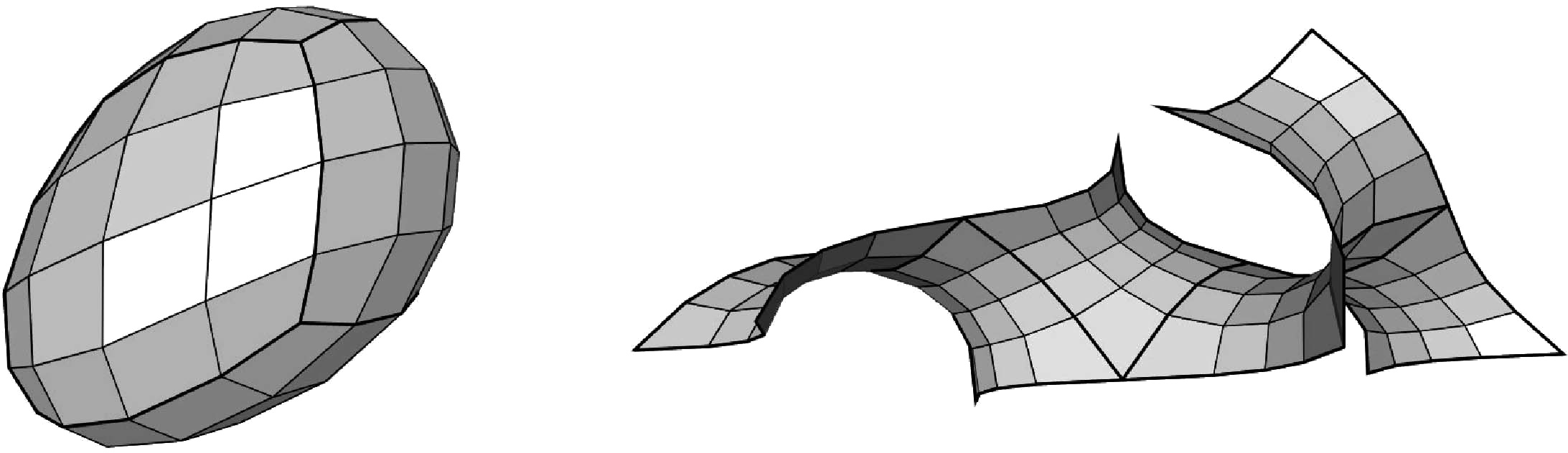
This result is analogous to the classical theorem of Christoffel [8] in the theory of smooth minimal surfaces. Figure 4 presents an example of a discrete minimal surface $m$ constructed as the Christoffel dual of its Gauss image $s$, which is a discrete Koenigs net.

The statement about surfaces with nonvanishing constant mean curvature resembles the corresponding facts of the classical theory.

Theorem 14.

A pair $(m,s)$ has constant mean curvature $H_{0}$ if and only if $m$ is a discrete Koenigs net and its parallel $m^{1/H_{0}}$ is the Christoffel dual of $m$:

$$m^{*}=m+\frac{1}{H_{0}}s.$$

The mean curvature of this parallel surface $(m+H_{0}^{-1}s,-s)$ (with the reversed Gauss map) is also constant and equal to $H_{0}$. The mid-surface $m+(2H_{0})^{-1}s$ has constant positive Gaussian curvature $K_{0}=4H_{0}^{2}$ with respect to the same Gauss map $s$.

• We have the equivalence

  $$A(m,s)=-H_{0}A(m)\ \iff\ A\Big{(}m,m+\frac{1}{H_{0}}s\Big{)}=0\ \iff\ m^{*}=m+\frac{1}{H_{0}}s.$$

  For the Gaussian curvature of the mid-surface we get

  $$K_{\frac{1}{2H_{0}}}=\frac{A(s)}{A(m+\frac{1}{2H_{0}}s)}=\frac{A(s)}{A(m)+{1\over H_{0}}A(m,s)+({1\over 2H_{0}})^{2}A(s)}=4H_{0}^{2}.$$

  ∎

It turns out that all surfaces parallel to a surface with constant curvature have remarkable curvature properties, in complete analogy to the classical surface theory. In particular they are linear Weingarten (For circular surfaces this was shown in [20]).

Theorem 15.

Let $(m,s)$ be a polyhedral surface with constant mean curvature and its Gauss map. Consider the family of parallel surfaces $m^{t}=m+ts$. Then for any $t$ the pair $(m^{t},s)$ is linear Weingarten, i.e., its mean and Gaussian curvatures $H_{t}$ and $K_{t}$ satisfy a linear relation

(12) $$\alpha H_{t}+\beta K_{t}=1$$

with constant coefficients $\alpha,\beta$.

• Denote by $H$ and $K$ the curvatures of the basic surface $(m,s)$ with constant mean curvature. Let us compute the curvatures $H_{t}$ and $K_{t}$ of the parallel surface $(m+ts,s)$. We have

  $$\dfrac{A(m+(t+\delta)s)}{A(m+ts)}=\dfrac{1-2H(t+\delta)+K(t+\delta)^{2}}{1-2Ht+Kt^{2}}$$

  $$=1-2\delta\dfrac{H-Kt}{1-2Ht+Kt^{2}}+\delta^{2}\dfrac{K}{1-2Ht+Kt^{2}}=1-2H_{t}\delta+K_{t}\delta^{2}.$$

  The last identity treats $m+(t+\delta)s$ as a parallel surface of $m+ts$. Thus,

  $$H_{t}=\frac{H-Kt}{1-2Ht+Kt^{2}},\quad K_{t}=\frac{K}{1-2Ht+Kt^{2}}.$$

  Note that $H$ is independent of the face, whereas $K$ is varying. Therefore, with the above values for $H_{t}$ and $K_{t}$, relation (12) is equivalent to $\frac{\alpha H}{1-2Ht}=\frac{\beta-\alpha t}{t^{2}}=1,$ which implies

  $$\alpha=\frac{1}{H}-2t,\quad\beta=\frac{t}{H}-t^{2}.$$

  ∎

We see that any discrete Koenigs net $m$ can be extended to a minimal or to a constant mean curvature net by an appropriate choice of the Gauss map $s$. Indeed,

• $(m,s)$ is minimal for $s=m^{*}$;

• $(m,s)$ has constant mean curvature for $s=m^{*}-m$.

However, $s$ defined in such generality can lead us too far away from the smooth theory. It is natural to look for additional requirements which bring it closer to the Gauss map of a surface. These are exactly three cases of special Gauss images of Section 2.

Cases with canonical Gauss image

For a polyhedral surface $m$ which has a face offset $m^{\prime}$ at distance $d>0$ (i.e., $m$ is a conical mesh) the Gauss image $s=(m^{\prime}-m)/d$ is uniquely defined even without knowledge of $m^{\prime}$, provided consistent orientation is possible. This is because $s$ is tangentially circumscribed to $S^{2}$ and there is only one way we can parallel translate the faces of $m$ such that they are in oriented contact with $S^{2}$. The same is true if $m$ has an edge offset, because an $n$-tuple of edges emanating from a vertex ($n\geq 3$) can be parallel translated in only one way so as to touch $S^{2}$.

It follows that for both cases a canonical Gauss image and canonical curvatures are defined. In case of an edge offset much more is known about the geometry of $s$. E.g. we can express the edge length of $s$ in terms of data read off from $m$ (see Figure 5). The edges emanating from a vertex $s_{i}$ are contained in $s_{i}$’s tangent cone, which has some opening angle $\omega_{j}$. By parallelity of edges we can determine $\omega_{j}$ from the mesh $m$ alone. The ratio between edge length in the mesh and edge length in the Gauss image determines the curvature: $\kappa_{i,j}=\pm(\cot\omega_{i}+\cot\omega_{j})/\|m_{i}-m_{j}\|$ (we skip discussion of the sign).

\begin{overpic}[width=130.08731pt]{fig/koebeklein} \put(59.0,20.0){\hbox to0.0pt{\hss{$c_{i}$}}} \put(50.0,71.0){$c_{j}$} \put(92.0,10.0){$s_{i}$} \end{overpic}

Figure 5. A Koebe polyhedron $s$. The tangent cone from each vertex $s_{i}$ touches $S^{2}$ along a circle $c_{i}$. These circles form a packing, touching each other in the points where the edges touch $S^{2}$. It follows that the edge lengths are related to the opening angles $\omega_{i}$ of said cones: We have $\|s_{i}-s_{j}\|=\cot\omega_{i}+\cot\omega_{j}$.

7. Curvature of principal contact element nets. Circular minimal and cmc surfaces

In this section we are dealing with the case when the Gauss image $s$ lies in the two-sphere $S^{2}$, i.e., is of unit length, $\|s\|=1$. Our main example is the case of quadrilateral surfaces with regular combinatorics, called Q-nets. In this case a polyhedral surface $m$ with its parallel Gauss map $s$ is described by a map

$$(m,s):\mathbb{Z}^{2}\to\mathbb{R}^{3}\times{S}^{2}.$$

It can be canonically identified with a contact element net

$$(m,{\mathcal{P}}):\mathbb{Z}^{2}\to\{{\rm contact\ elements\ in}\ \mathbb{R}^{3}\},$$

where $\mathcal{P}$ is the oriented plane orthogonal $s$. We will call the pair $(m,s)$ also a contact element net. Recall that according to [5] a contact element net is called principal if neighboring contact elements $(m,{\mathcal{P}})$ share a common touching sphere. This condition is equivalent to the existence of focal points for all elementary edges $(n,n^{\prime})$ of the lattice $\mathbb{Z}^{2}\ni n,n^{\prime}$, which are solutions to

$$(m+ts)(n)=(m+ts)(n^{\prime})$$

for some $t$.

Theorem 16.

Let $m:\mathbb{Z}^{2}\to\mathbb{R}^{3}$ be a Q-net with a parallel unit Gauss map $s:\mathbb{Z}^{2}\to S^{2}$. Then $m$ is circular, and $(m,s)$ is a principal contact element net. Conversely, for a principal contact element net $(m,s)$, the net $m$ is circular and $s$ is a parallel Gauss map of $m$.

• The circularity of $m$ follows from the simple fact that any quadrilateral with edges parallel to the edges of a circular quadrilateral is also circular. Consider an elementary cube built by two parallel quadrilaterals of the nets $m$ and $m+s$. All the side faces of this cube are trapezoids, which implies that the contact element net $(m,s)$ is principal. ∎

Figure 6. Parallel Q-nets $m$ and $m+s$ with the unit Gauss map $s$. All the nets are circular. The pair $(m,s)$ constitutes a principal contact element net.

The mean and the Gauss curvatures of the principal contact element nets $(m,s)$ are defined by formulas (8).

Proposition 9 obviously implies:

Corollary 17.

For a circular quad mesh $m$, principal curvatures exist w.r.t. any Gauss image $s$ inscribed in $S^{2}$.

Recall also that circular Koenigs nets are identified in [7, 6] as the discrete isothermic surfaces defined originally in [3] as circular nets with factorizable cross-ratios.

Both minimal and constant mean curvature principal contact element nets are defined as in Section 6. It is remarkable that the classes of circular minimal and cmc surfaces which are obtained via our definition of mean curvature turn out to be equivalent to the corresponding classes originally defined as special isothermic surfaces characterized by their Christoffel transformations. Since circular Koenigs nets are isothermic nets, from Theorem 13 we recover the original definition of discrete minimal surfaces from [3].

Corollary 18.

A principal contact element net $(m,s):\mathbb{Z}^{2}\to\mathbb{R}^{3}\times S^{2}$ is minimal if and only if the net $s:\mathbb{Z}^{2}\to S^{2}$ is isothermic and $m=s^{*}$ is its Christoffel dual.

Similarly, Theorem 14 in the circular case implies that the discrete surfaces with constant mean curvature of [10, 4] fit into our framework.

Corollary 19.

A principal contact element net $(m,s):\mathbb{Z}^{2}\to\mathbb{R}^{3}\times S^{2}$ has constant mean curvature $H_{0}\neq 0$ if and only if the circular net $m$ is isothermic and there exists its dual discrete isothermic surface $m^{*}:\mathbb{Z}^{2}\to\mathbb{R}^{3}$ at constant distance $|m-m^{*}|=\frac{1}{H_{0}}$. The unit Gauss map $s$ which determines the principal contact element net $(m,s)$ is given by

(13) $$s=H_{0}(m^{*}-m).$$

The principal contact element net of the parallel surface $(m+\frac{1}{H_{0}},-s)$ also has constant mean curvature $H_{0}$. The mid-surface $(m+\frac{1}{2H_{0}},s)$ has constant Gaussian curvature $4H_{0}^{2}$.

• Only the “if” part of the claim may require some additional consideration. If the discrete isothermic surfaces $m$ and $m^{*}$ are at constant distance $1/H_{0}$, then the map $s$ defined by (13) maps into $S^{2}$ and is thus circular. Again, as in the proof of Theorem 16, this implies that the contact element net $(m,s)$ is principal. Its mean curvature is given by

  $$-\frac{A(m,s)}{A(m,m)}=-\frac{A(m,H_{0}(m^{*}-m))}{A(m,m)}=H_{0}.$$

  ∎

7.1. Minimal s-isothermic surfaces

We now turn our attention to the discrete minimal surfaces $m$ of [1], which arise by a Christoffel duality from a polyhedron $s$ which is midscribed to a sphere (a Koebe polyhedron). As Koebe polyhedra are up to Möbius transformations determined by their combinatorics, a passage to the limit allows us to determine in this way the shape of smooth minimal surface from the combinatorics of the Gauss image of its network of principal curvature lines.

The Christoffel duality construction of [1] is applied to each face of $s$ separately. We consider a polygon $P=(p_{0},\dots,p_{n-1})$ with $n$ even and incircle of radius $\rho$. We introduce the points $q_{i}$ where the edge $p_{i-1}p_{i}$ touches the incircle and identify the plane of $P$ with the complex numbers. In the notation of Figure 7 the passage to the dual polygon $P^{*}$ is effected by changing the vectors $a_{i}=q_{2i}-z$, $b_{i}=q_{2i+1}-z$, $a^{\prime}_{i}=p_{2i}-q_{2i+1}$, $b^{\prime}_{i}=p_{i}-q_{i}$. Apart from multiplication with the factor $\pm\rho^{2}$, the corresponding vectors which define $P^{*}$ are given by

(14) $$a_{j}^{*}=(-1)^{j}/\overline{a_{j}},\quad b_{j}^{*}=-(-1)^{j}/\overline{b_{j}},\quad a_{j}^{\prime*}=(-1)^{j}/\overline{a_{j}^{\prime}},\quad b_{j}^{\prime*}=-(-1)^{j}/\overline{b_{j}^{\prime}}.$$

The sign in the factor $\pm\rho^{2}$ depends on a certain labeling of vertices. The consistency of this construction and the passage to a branched covering in the case of odd $n$ is discussed in [1]. For us it is important that both $P$ and $P^{*}$ occur as concatenation of quadrilaterals:

(15) $$P_{j}=(p_{j-1}q_{j}p_{j}q_{j})\ \mbox{for}\ j=0,\dots,n-1\implies P=P_{1}\oplus\ldots\oplus P_{n-1},$$

and the same for the starred (dual) entities. The main result is the following:

\begin{overpic}[height=151.76964pt]{fig/chrkr1} \put(70.0,51.0){$a_{0}$} \put(95.0,60.0){$b^{\prime}_{0}$} \put(50.0,49.0){\hbox to0.0pt{\hss{$z$}}} \put(53.0,60.0){$b_{0}$} \put(70.0,94.0){\hbox to0.0pt{\hss{$a^{\prime}_{0}$}}} \put(95.0,48.0){$q_{0}$} \put(46.0,90.0){\hbox to0.0pt{\hss{$q_{1}$}\hss}} \put(70.0,62.0){\hbox to0.0pt{\hss{$P_{0}$}\hss}} \put(33.0,56.0){\hbox to0.0pt{\hss{$P_{1}$}\hss}} \put(35.0,28.0){\hbox to0.0pt{\hss{$P_{2}$}\hss}} \put(68.0,24.0){\hbox to0.0pt{\hss{$P_{3}$}\hss}} \put(93.0,101.0){\hbox to0.0pt{\hss{$p_{0}$}\hss}} \put(5.0,81.0){\hbox to0.0pt{\hss{$p_{1}$}\hss}} \put(22.0,10.0){\hbox to0.0pt{\hss{$p_{2}$}}} \put(94.0,0.0){$p_{3}$} \end{overpic}    \begin{overpic}[height=151.76964pt]{fig/chrkr2} \put(75.0,51.0){\hbox to0.0pt{\hss{$1/\overline{a_{0}}$}\hss}} \put(99.0,50.0){$q_{0}^{*}$} \put(99.0,30.0){$-1/\overline{b^{\prime}_{0}}$} \put(77.0,7.0){$1/\overline{a^{\prime}_{0}}$} \put(62.0,30.0){\hbox to0.0pt{\hss{$-1/\overline{b_{0}}$}}} \put(59.0,50.0){\hbox to0.0pt{\hss{$z^{*}$}}} \put(98.0,12.0){$p_{0}^{*}$} \put(33.0,0.0){\hbox to0.0pt{\hss{$p_{1}^{*}$}}} \put(65.0,5.0){$q_{1}^{*}$} \put(10.0,100.0){$p_{2}^{*}$} \put(95.0,84.0){\hbox to0.0pt{\hss{$p_{3}^{*}$}\hss}} \put(77.0,62.0){\hbox to0.0pt{\hss{$P_{3}^{*}$}\hss}} \put(40.0,60.0){\hbox to0.0pt{\hss{$P_{2}^{*}$}\hss}} \put(44.0,20.0){\hbox to0.0pt{\hss{$P_{1}^{*}$}\hss}} \put(75.0,30.0){\hbox to0.0pt{\hss{$P_{0}^{*}$}\hss}} \end{overpic}

Figure 7. Christoffel duality construction for $s$-isothermic surfaces applied to a quadrilateral $P$ with incircle. Corresponding sub-quadrilaterals $P_{j}$, $P_{j}^{*}$ have vanishing mixed area.

Theorem 20.

A discrete s-isothermic minimal surface $m$ according to [1] (Christoffel dual of a Koebe polyhedron $s$) has vanishing mean curvature. Every face $f$ has principal curvatures $\kappa_{1,f},\kappa_{2,f}=-\kappa_{1,f}$.

• We first show that for all $j$, $A(P_{j},P_{j}^{*})=0$. This can be derived from [1] where it is shown that $P_{j}$ and $P_{j}^{*}$ are dual quads in the sense of discrete isothermic surfaces [3]. Discrete isothermic surfaces are circular Koenigs nets [6], i.e., the quadrilaterals $P_{j}$ and $P_{j}^{*}$ are Christoffel dual in the sense of Definition 11.

  We can see this also in an elementary way which for $\rho=1$ is illustrated by Figure 7: The angle $\alpha_{i}=\sphericalangle(q_{i},z,p_{i})$ occurs also in the isosceles triangle $q_{i}^{*}z^{*}q_{i+1}^{*}$, so non-corresponding diagonals in $P_{i},P_{i}^{*}$ are parallel. By Theorem 12, $A(P_{i},P_{i}^{*})=0$.

  Lemma 4 now implies that $A(P,P^{*})=\sum A(P_{j},P_{j}^{*})=0$. Thus all faces of $m$ (i.e., the $P^{*}$’s of the previous discussion) have vanishing mixed area with respect to $s$. As the faces of $s$ are strictly convex, Prop. 9 shows that principal curvatures exist. ∎

7.2. Discrete surfaces of rotational symmetry

It is not difficult to impose the condition of constant mean or Gaussian curvature on discrete surfaces with rotational symmetry. In the following we briefly discuss this interesting class of examples.

We first consider quadrilateral meshes with regular grid combinatorics generated by iteratively applying a rotation about the $z$ axis to a meridian polygon contained in the $xz$ plane. Such surfaces have e.g. been considered by [12].

The vertices of the meridian polygon are assumed to have coordinates $(r_{i},0,h_{i})$, where $i$ is the running index. The Gauss image of this polyhedral surface shall be generated in the same way, from the polygon with vertices $(r_{i}^{*},0,h_{i}^{*})$. Note that parallelity implies

(16) $${r_{i+1}-r_{i}\over h_{i+1}-h_{i}}={r_{i+1}^{*}-r_{i}^{*}\over h_{i+1}^{*}-h_{i}^{*}}.$$

Figure 8 illustrates such surfaces. All faces being trapezoids, it is elementary to compute mean and Gaussian curvatures $H^{(i)}$, $K^{(i)}$ of the faces bounded by the $i$-th and $(i+1)$-st parallel. It turns out that the angle of rotation is irrelevant for the curvatures:

(17) $$H^{(i)}={r_{i}r_{i}^{*}-r_{i+1}r_{i+1}^{*}\over r_{i+1}^{2}-r_{i}^{2}},\quad K^{(i)}={r_{i+1}^{*2}-r_{i}^{*2}\over r_{i+1}^{2}-r_{i}^{2}}.$$

The principal curvatures associated with these faces have the values

(18) $$\kappa_{1}^{(i)}={r_{i+1}^{*}+r_{i}^{*}\over{r_{i+1}+r_{i}}},\quad\kappa_{2}^{(i)}={r_{i+1}^{*}-r_{i}^{*}\over{r_{i+1}-r_{i}}}.$$

The interesting fact about these formulae is that the coordinates $h_{i}$ do not occur in them. Any functional relation involving the curvatures, and especially a constant value of any of the curvatures, leads to a difference equation for $(r_{i})_{i\in{\mathbb{Z}}}$. For example, given an arbitrary Gauss image $(r_{i}^{*},0,h_{i}^{*})$ and the mean curvature function $H^{(i)}$ defined on the faces (which are canonically associated with the edges of the meridian curve) the values $r_{i}$ of the surface are determined by the difference equation (17) an an initial value $r_{0}$. Further the values $h_{i}$ follow from the parallelity condition (16).

A meridian curve of a smooth surface of revolution does not intersect the rotation axis, and the Gauss map is spherical. Discrete analogues of such surfaces with a Gauss map $s\in S^{2}$ and prescribed curvature are determined by the values $(h^{*}_{i})_{i\in{\mathbb{Z}}}$ lying in the interval $(-1,1)$, and an initial value $r_{0}$. The values $r^{*}_{i}=(1-{h^{*}_{i}}^{2})^{1/2}$ should be chosen positive.

\begin{overpic}[height=91.0631pt]{fig/relmin1} \put(5.0,5.0){\hbox to0.0pt{\hss{$s$}}} \put(85.0,17.0){$m$} \end{overpic}

\begin{overpic}[height=143.09538pt]{fig/gaussian30} \put(8.0,57.0){\hbox to0.0pt{\hss{$s^{\prime}$}}} \put(85.0,20.0){$m^{\prime}$} \end{overpic}

Figure 8. Left: A polyhedral surface $m$ which is a minimal surface w.r.t. to the Gaussian image $s$. Right: A polyhedral surface $m^{\prime}$ of constant Gaussian curvature w.r.t. the Gauss image $s^{\prime}$ (discrete pseudosphere).

Remark 3.

The generation of a surface $m$ and its Gauss image $s$ by applying $k$-th powers of the same rotation to a meridian polygon (assuming axes of $m$ and $s$ are aligned) is a special case of applying a sequence of affine mappings, each of which leaves the axis fixed. It is easy to see that Equations (17) and (18) are true also in this more general case.

Remark 4.

While the formula for $\kappa_{2}$ given by (18) is the usual definition of curvature for a planar curve, the formula for $\kappa_{1}$ can be interpreted as Meusnier’s theorem. This is seen as follows: The curvature of the $i$-th parallel circle is given some average value of $1/r$ (in this case, the harmonic mean of $1/r_{i}$ and $1/r_{r+1}$). The sine of the angle $\alpha$ enclosed by the parallel’s plane and the face under consideration is given by an average value of $r^{*}$ (this time, an arithmetic mean). By Meusnier, the normal curvature “$\sin\alpha\cdot{1\over r}$” of the parallel equals the principal curvature $\kappa_{1}$, in accordance with (18).

Example 1.

The mean curvature of faces given by (17) vanishes if and only if $r_{i+1}:r_{i}=r_{i}^{*}:r_{i+1}^{*}$. This condition is converted into the first order difference equation

(19) $$\Delta\ln r_{i}=-\Delta\ln r^{*}_{i}\quad(i\in{\mathbb{Z}}),$$

where $\Delta$ is the forward difference operator. It is not difficult to see that the corresponding differential equation $(\ln r)^{\prime}=-(\ln r^{*})^{\prime}$ is fulfilled by the catenoid: With the meridian $(t,\cosh t)$ and the unit normal vector $(-\tanh t,1/\cosh t)$ we have $r(t)=\cosh t$ and $r^{*}(t)=1/\cosh t$. We therefore like to denote discrete surfaces fulfilling (19) discrete catenoids (see Figure 8, left).

Example 2.

A discrete surface of constant Gaussian curvature $K$ obeys the difference equation $K\Delta(r_{i}^{2})=\Delta(r_{i}^{*2})$. Figure 8, right illustrates a solutions.

7.3. Discrete surfaces of rotational symmetry with constant mean curvature and elliptic billiards

There exists a nice geometric construction of discrete surfaces of rotational symmetry with constant mean curvature, which we obtained jointly with Tim Hoffmann. This is a discrete version of the classical Delaunay rolling ellipse construction for surfaces of revolution with constant mean curvature (Delaunay surfaces).

Play an extrinsic billiard around an ellipse $E$. A trajectory is a polygonal curve $P_{1},P_{2},\ldots$ such that the intervals $[P_{i},P_{i+1}]$ touch the ellipse $E$ and consecutive triples of vertices $P_{i-1},P_{i},P_{i+1}$ are not collinear (see Figure 10). Let us connect the vertices $P_{i}$ to the focal point $B$, and roll the trajectory $P_{1},P_{2},\ldots$ to a straight line $\ell$, mapping the triangles $BP_{i}P_{i+1}$ of Figure 10 isometrically to the triangles $B_{i}P_{i}P_{i+1}$ of Figure 10. We use the same notations for the vertices of the billiard trajectory and their images on the straight line, and the points $B_{i}$ are chosen in the same half-plane of $\ell$. Thus we have constructed a polygonal curve $B_{1},B_{2},\ldots$ . Applying the same construction to the second focal point $A$ we obtain another polygonal curve $A_{1},A_{2},\ldots$, chosen to lie in another half-plane of $\ell$.

Figure 9. An external elliptic billiard. The trajectory $\{P_{i}\}_{i\in{\mathbb{Z}}}$ is tangent to an ellipse.

Figure 10. A discrete cmc surface with rotational symmetry generated from an elliptic billiard.

Let us consider discrete surfaces $m$ and $\widetilde{m}$ with rotational symmetry axis $\ell$ generated by the meridian polygons constructed above: $m_{i}=B_{i}$, $\widetilde{m}_{i}=A_{i}$. They are circular surfaces which one can provide with the same Gauss map $s_{i}:=m_{i}-\widetilde{m}_{i}$.

Theorem 21.

Let $P_{1},P_{2},\ldots$ be a trajectory of an extrinsic elliptic billiard with the focal points $A,B$. Let $m,\widetilde{m}$ be the circular surfaces with rotational symmetry generated by the discrete rolling ellipse construction in Figures 10, 10: $m_{i}=B_{i}$, $\widetilde{m}_{i}=A_{i}$. Both surfaces $(m,s)$ and $(\widetilde{m},-s)$ with the Gauss map $s=m-\widetilde{m}$ have constant mean curvature $H$, where $1/H=|A_{1}B|$ equals twice the major axis of the ellipse (see Figure 10).

• The sum of the distances from a point of an ellipse to the focal points is independent of the point, i.e.,

  $$l:=|A_{i}B_{i}|$$

  is independent of $i$. Due to the equal angle lemma of Figure 11 we have equal angles $\beta:=\angle P_{1}P_{2}A_{1}=\angle BP_{2}P_{3}$ and $\gamma:=\angle P_{1}P_{2}B=\angle P_{3}P_{2}A_{2}$ in Figure 10. Thus $P_{2}$ in Figure 10 is the intersection point of the straight lines $(A_{1}B_{2})\cap(B_{1}A_{2})$. Similar triangles $\triangle P_{2}A_{1}A_{2}\sim\triangle P_{2}B_{2}B_{1}$ imply parallel edges $(A_{1}A_{2})\parallel(B_{1}B_{2})$. This yields the proportionality $r_{i}/r_{i+1}=r^{\prime}_{i+1}/r^{\prime}_{i}$ for the distances $r$ to the axis $\ell$. For the mean curvature of the surface $m$ with the Gauss image $s=m-\widetilde{m}$ we obtain from (17):

  $$H=\frac{1}{l}\frac{r_{i}(r^{\prime}_{i}-r_{i})-r_{i+1}(r^{\prime}_{i+1}-r_{i+1})}{r_{i+1}^{2}-r_{i}^{2}}=\frac{1}{l}.$$

  The surface $\widetilde{m}$ is the parallel cmc surface of Corollary 19. ∎

Figure 11. The angles between the tangent directions and the directions to the focal points of an ellipse are equal.

If the vertices of the trajectory $P_{1},P_{2},\ldots$ lie on an ellipse $E^{\prime}$ confocal with $E$, then it is a classical reflection billiard in the ellipse $E^{\prime}$ (see for example [23]). The sum

$$d:=|AP_{i}|+|BP_{i}|$$

is independent of $i$. The quadrilaterals $A_{i}A_{i+1}B_{i+1}B_{i}$ in Figure 10 have equal diagonals, i.e., are trapezoids. The product of the lengths of their parallel edges is independent of $i$:

(20) $$|A_{i}A_{i+1}||B_{i}B_{i+1}|=d^{2}-l^{2}.$$

As we have shown in the proof of Theorem 21, $r_{i}r^{\prime}_{i}$ is another product independent of $i$. An elementary computation gives the same result for the cross-ratios of a faces of the discrete surfaces $m$ and $\widetilde{m}$:

$$q=-\frac{1}{\sin^{2}\alpha}\frac{|A_{i}A_{i+1}||B_{i}B_{i+1}|}{r_{i}r^{\prime}_{i}},$$

where $2\alpha$ is the rotation symmetry angle of the surface. We see that $q$ is the same for all faces of the surfaces $m$ and $\widetilde{m}$.

We have derived the main result of [11].

Corollary 22.

Let $P_{1},P_{2},\ldots$ be a trajectory of a classical reflection elliptic billiard, and $m,\widetilde{m}$ be the discrete surfaces with rotational symmetry generated by the discrete rolling ellipse construction as in Theorem 21. Both these surfaces have constant mean curvature and constant cross-ratio of their faces.

The discrete rolling construction applied to hyperbolic billiards also generates discrete cmc surfaces with rotational symmetry.

8. Concluding remarks

We would like to mention some topics of future research. We have treated curvatures of faces and of edges. It would be desirable to extend the developed theory to define curvature also at vertices. A large area of research is to extend the present theory to the semidiscrete surfaces which have recently found attention in the geometry processing community, and where initial results have already been obtained.

References

- [1] A. I. Bobenko, T. Hoffmann, and B. Springborn, Minimal surfaces from circle patterns: Geometry from combinatorics, Ann. of Math. 164 (2006), 231–264.
- [2] A. I. Bobenko, S. P., J. M. Sullivan, and G. M. Ziegler (eds.), Discrete differential geometry, Oberwolfach Seminars, vol. 38, Birkhäuser, Basel, 2008.
- [3] A. I. Bobenko and U. Pinkall, Discrete isothermic surfaces, J. Reine Angew. Math. 475 (1996), 187–208.
- [4] A. I. Bobenko and U. Pinkall, Discretization of surfaces and integrable systems, Discrete integrable geometry and physics (A. I. Bobenko and R. Seiler, eds.), Oxford Lecture Ser. Math. Appl., vol. 16, Oxford Univ. Press, 1999, pp. 3–58.
- [5] A. I. Bobenko and Yu. Suris, On organizing principles of discrete differential geometry. Geometry of spheres, Russian Math. Surveys 62 (2007), no. 1, 1–43.
- [6] by same author, Discrete differential geometry. Integrable structure, Graduate Studies in Math., no. 98, American Math. Soc., 2008.
- [7] by same author, Discrete Koenigs nets and discrete isothermic surfaces, Int. Math. Res. Not. (2009), to appear.
- [8] E. Christoffel, Ueber einige allgemeine Eigenschaften der Minimumsflächen, J. Reine Angew. Math. 67 (1867), 218–228.
- [9] A. P. Fordy and J. C. Wood (eds.), Harmonic maps and integrable systems, Aspects of Mathematics, vol. E23, Vieweg, Braunschweig, 1994.
- [10] U. Hertrich-Jeromin, T. Hoffmann, and U. Pinkall, A discrete version of the Darboux transform for isothermic surfaces, Discrete integrable geometry and physics (A. I. Bobenko and R. Seiler, eds.), Clarendon Press, Oxford, 1999, pp. 59–81.
- [11] T. Hoffmann, Discrete rotational cmc surfaces and the elliptic billiard, Mathematical Visualization (H.-C. Hege and K. Polthier, eds.), Springer, Berlin, 1998, pp. 117–124.
- [12] B. G. Konopelchenko and W. K. Schief, Trapezoidal discrete surfaces: geometry and integrability, J. Geometry Physics 31 (1999), 75–95.
- [13] U. Pinkall and K. Polthier, Computing discrete minimal surfaces and their conjugates, Experiment. Math. 2 (1993), no. 1, 15–36.
- [14] H. Pottmann, P. Grohs, and B. Blaschitz, Edge offset meshes in Laguerre geometry, Adv. Comput. Math. (2009), to appear.
- [15] H. Pottmann, Y. Liu, J. Wallner, A. I. Bobenko, and W. Wang, Geometry of multi-layer freeform structures for architecture, ACM Trans. Graphics 26 (2007), no. 3, #65, 11 pp.
- [16] H. Pottmann and J. Wallner, The focal geometry of circular and conical meshes, Adv. Comp. Math 29 (2008), 249–268.
- [17] C. Rogers and W. K. Schief, Bäcklund and Darboux transformations. Geometry and modern applications in soliton theory, Cambridge Texts in Applied Mathematics, Cambridge University Press, Cambridge, 2002.
- [18] R. Sauer, Parallelogrammgitter als Modelle pseudosphärischer Flächen, Math. Z. 52 (1950), 611–622.
- [19] W. K. Schief, On the unification of classical and novel integrable surfaces. II. Difference geometry, R. Soc. Lond. Proc. Ser. A 459 (2003), 373–391.
- [20] W. K. Schief, On a maximum principle for minimal surfaces and their integrable discrete counterparts, J. Geom. Physics 56 (2006), 1484–1495.
- [21] R. Schneider, Convex bodies: the Brunn-Minkowski theory, Encyclopedia of Mathematics and its Applications, vol. 44, Cambridge University Press, 1993.
- [22] U. Simon, A. Schwenck-Schellschmidt, and H. Viesel, Introduction to the affine differential geometry of hypersurfaces. Lecture notes, Science Univ. Tokyo, 1992.
- [23] S. Tabachnikov, Geometry and billiards, Student Mathematical Library, no. 30, American Math. Soc., 2005.
- [24] W. Wunderlich, Zur Differenzengeometrie der Flächen konstanter negativer Krümmung, Sitz. Öst.. Akad. Wiss. Math.-Nat. Kl. 160 (1951), 39–77.