Spontaneous waves in muscle fibres
Abstract
Mechanical oscillations are important for many cellular processes, e.g., the beating of cilia and flagella or the sensation of sound by hair cells. These dynamic states originate from spontaneous oscillations of molecular motors. A particularly clear example of such oscillations has been observed in muscle fibers under non-physiological conditions. In that case, motor oscillations lead to contraction waves along the fiber. By a macroscopic analysis of muscle fiber dynamics we find that the spontaneous waves involve non-hydrodynamic modes. A simple microscopic model of sarcomere dynamics highlights mechanical aspects of the motor dynamics and fits with the experimental observations.
1 Introduction
Oscillations are a common phenomenon in biological systems. Even on a cellular level oscillatory dynamics is widespread [1]. Examples are provided by circadian rhythms through which cells anticipate the changes of day and night [2], by the Min-oscillations in the bacterium Escherichia coli that help to select the cell center as the division site [3], by hair bundle oscillations in auditory hair cells [4], and by the beating patterns of cilia and flagella that are crucial for the transport of mucus and propel microorganisms [5].
The latter are examples of mechanical oscillations that involve molecular motors [5, 6, 7]. These proteins are able to transform chemical energy into mechanical work. The chemical energy is provided by the hydrolysis of Adenosine-Tri-Phosphate (ATP) which results in Adenosine-Di-Phosphate (ADP) and inorganic phosphate (Pi). Motor proteins can catalyze this reaction and concomitantly undergo conformational changes. By this motion they can translate directionally along polar protein filaments and transport cargos or generate forces. Examples are myosin motors that interact with actin filaments and kinesins or dyneins that interact with microtubules. The polarity of actin filaments and microtubules results from structural differences between the two ends of a filament and a microtubule and determines the direction of motion of a motor.
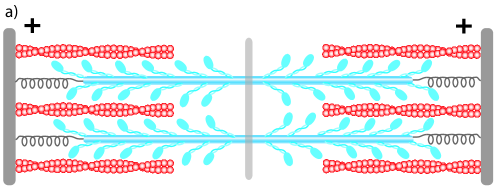
On theoretical grounds it had been suggested that ensembles of molecular motors connected to elastic elements can generate spontaneous oscillations through a Hopf-bifurcation [8]. It has been proposed that such mechanical oscillations are at the origin of flagellar and ciliary beats [9, 10, 11] and of mitotic spindle oscillations during asymmetric cell divisions [12]. A striking evidence of spontaneous oscillations caused by molecular motors is provided by oscillations of muscle fibers that have been studied in the past 20 years by Ishiwata and collaborators [13, 14, 15, 16, 17, 18, 19, 20]. Muscle fibers are chains of sarcomeres, the elementary force generating units of skeletal and cardiac muscle [5], see Fig. 1 for an illustration. In a sarcomere actin filaments and filaments consisting of many myosin motor molecules are arranged in such a way that activation of the motors leads to contraction of the structure. Its integrity is maintained by passive elastic elements.
Spontaneous sarcomere oscillations are observed under constant, but non-physiological chemical conditions [13]. Remarkably, the oscillations exists even in reconstituted muscle fibers that contain only essential structural elements like actin, myosin, and scaffolding proteins, but no regulatory elements [19]. Depending on the external conditions and applied forces, the oscillations of sarcomeres in a muscle fiber can be either synchronous or asynchronous [18, 17]. Under appropriate conditions, contraction waves traveling along the muscle fiber can be observed [13, 14, 20].
Theoretical work on this system has so far focused on synchronization effects of chains of coupled Hopf-oscillators [21]. In that analysis, synchronization effects due a global coupling of oscillatory elements through a mass have been studied. In particular, a rich phase diagram of synchronous and asynchronous states was found. In another study, gradients in sarcomere properties where suggested to cause synchronization between adjacent sarcomeres which ultimately yields coherent contraction waves [22]. The existence of such a gradient is currently not supported by experiments. A comprehensive theoretical account of the experiments by Ishiwata et al. is currently not available.
We present in this work a study of the dynamics of muscle fibers using two complementary approaches. Phenomenological descriptions of active polar gels provide a general framework for studying the dynamics of motor filament systems [23, 24, 25, 26] and have been successfully applied, for example, to describe essential features of the lamellipodia of crawling cells [27]. We will start therefore in the next section by developing a hydrodynamic theory of muscle fibers. As will be shown, this description fails to yield oscillatory solutions. In the subsequent section we will consider a microscopic model of muscle sarcomeres in which spontaneous oscillations are a consequence of load dependent detachment rates of motors from filaments. The corresponding model of a chain of sarcomeres is then shown to wholly reproduce the phenomenology of waves along muscle fibers. In the discussion, we compare the results of our theoretical analysis to experimental observations.
2 Hydrodynamic description of muscle fibres
Hydrodynamics is a systematic approach to assess dynamic phenomena of spatially extended systems in the limit of large wave-lengths and long time-scales. Formally, a hydrodynamic mode of wave-length relaxes with a characteristic time . In this limit, it is appropriate to make the assumption of local thermodynamic equilibrium [28]: In thought, the system is subdivided into volumes that are small compared to the large scale structures of interest and that are, at the same time, large enough to allow for a thermodynamic (equilibrium) description. Based in this assumption, a free energy can be defined for the full system which is out of equilibrium. The change with time of the free energy can be expressed as a sum of products of generalized forces and fluxes. Then, the fluxes are expressed in terms of the forces, where only terms of linear order are considered. The resulting description is purely phenomenological and only depends on the modes under consideration as well as the symmetries of the system.
We will apply this approach to muscle fibers, which will be considered as one-dimensional one-component complex fluids. First, we have to identify the hydrodynamic modes of the systems. In general, they are associated with conservation laws or broken continuous symmetries. The muscle fiber is an essentially one-dimensional system with the order of the actin and myosin filaments being fixed. Consequently the system does not offer any broken continuous symmetry. There are three conserved quantities: the fiber mass, momentum and energy. In experiments, the fluid surrounding the fiber essentially provides a heat bath such that temperature is constant and energy conservation is not an issue. Note, that this no longer holds for muscle, which heat up when active. Conservation of mass and momentum implies
| (1) |
where is the mass density along the fiber and its local velocity, and
| (2) |
In this expression the stress gives the momentum flux density and is an externally applied force. For the dynamic phenomena we consider, inertia is irrelevant, such that Eq. (2) reduces to a force-balance relation between internal stresses and external forces.
Under the assumption of local thermodynamic equilibrium, changes in the system’s free energy can be expressed as
| (3) |
It can thus be written as a sum of products, where in each product, a generalized flux is multiplied with its conjugate generalized force. In the present case, the fluxes are taken to be the stress and the rate of ATP-hydrolysis . The force conjugate to is the rate of strain , the force conjugate to the difference in chemical potentials of ATP and its hydrolysis products ADP and Pi, . Note, that since the density changes by relative sliding of actin filaments and motor filaments, we assume that the system is infinitely compressible. Consequently, the pressure vanishes.
In the next step, the generalized fluxes are expanded in terms of the generalized forces up to linear order. To this end the fluxes have to be separated into their reactive and their dissipative components. The dissipative component of a flux has the same sign with respect to time-reversal as its conjugate flux, the reactive component has the opposite sign. The corresponding changes in the free energy are thus, respectively, irreversible and reversible with respect to time-reversal. The respective components of a flux can be expanded only in terms of forces with the same behavior under time-reversal. With and , where the superscripts and discriminate between the reactive and the dissipative parts, respectively, we get
| (4) | |||||
| (5) | |||||
| (6) | |||||
| (7) |
The phenomenological coefficient accounts for the effects of an internal friction in the muscle fiber, while determines the rate of ATP-hydrolysis given a difference in chemical potentials . The coefficient is a measure of the contribution to the stress by active processes, i.e., the action of motors. The coefficients in front of the cross-terms must be equal up to a sign due to the Onsager relations.
Equations (4)-(7) provide the constitutive equations for an active fluid and thus take no account of the passive elastic response of a muscle fiber. Such a response, however, is expected in a passive fiber, , due to the elastic elements of sarcomeres, which help to maintain structural integrity. Consequently, on large time scales, one expects an elastic response also in the active case. The short time behavior in the passive case is somewhat more subtle. The motor molecules constantly detach from actin filaments and rebind. This dynamics leads to a viscous response of the system [29, 30]. Therefore, the passive system shows visco-elastic behavior. Note, that on very short time scales, bound motors will lead to an additional elastic response. We will neglect this contribution and consider only one relaxation time. In contrast to theories of active polar gels [24, 25], we thus have viscous behavior on short and elastic behavior on long time scales. We will model this behavior of the passive system by the Kelvin-Voigt model of a linear spring and a dashpot acting in parallel, such that the elastic and the viscous stresses simply add. The elastic part is given by , where is the equilibrium density and the elastic modulus. The elastic part must be added to the reactive component of the stress in Eq. (6).
For the analysis of the dynamic equations (4)-(7), we take a dependence of the active stress on the density into account: As the overlap between the actin filaments and the motor filaments increase, the active stress changes for constant . We therefore expand in terms of , while keeping only terms up to first order, . In the case that the only external force results from friction with the surrounding fluid, we write , where is the corresponding friction coefficient. Combining this expression with the dynamic equations for , the time evolution of deviations from the equilibrium distribution is determined up to linear order by
| (8) |
If , a perturbation of the equilibrium state will thus grow leading to a contracted state. The condition states essentially that the active stresses must be larger than the passive elastic stresses. Note, however, that the dynamic equation for the fiber density does not allow for wave solutions.
3 Microscopic model of muscle fibers
As we have seen in the previous section, the oscillation mechanism of muscle fibers involves non-hydrodynamic modes. In this section, we will propose a microscopic model of the dynamics of muscle fibers. First, we present the dynamics of a half-sarcomere and show that it is able to oscillate spontaneously. We then study the dynamics of a chain of such elements and compare it to the experimental observations on muscle fibers. Finally, we obtain the continuum limit of the chain and compare it to the description developed in the previous section.
3.1 The half-sarcomere
Muscle fibers are periodic structures. The elementary units are sarcomeres as illustrated in Fig. 1. A sarcomere consists of filaments of myosin-II motors and actin filaments with their plus-ends pointing outwards. By activation of the motors, the structure contracts. In addition to the active acto-myosin system, there are passive elastic elements affecting the dynamics of a sarcomere. Elasticity results from structural elements like the Z-disc, to which actin filaments are attached with their plus-ends, or from titin, a molecule extending through the whole length of a sarcomere and preventing it from falling apart upon stretching. From a dynamic point of view, the two halves of a sarcomere are identical, such that half-sarcomeres can be considered as the elementary units of a muscle fiber. We are now going to specify the dynamics of this structure.
3.1.1 The dynamic equations.
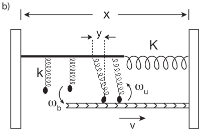
We approximate a half-sarcomere by the structure illustrated in Fig. 2. It consists of motors moving along a polar filament and a linear spring of stiffness . The motors are attached to a common backbone by springs of stiffness and extension . The motor filament as well as the polar filament are effective structures that result from averaging the parallel filaments in a sarcomere in the direction perpendicular to the sarcomere extension. The whole structure is immersed in a fluid of viscosity .
A motor in the overlap region of the motor filament and the polar filament stochastically binds to and unbinds from the polar filament with rates and , respectively. The binding and unbinding rates depend in general on the force applied to the motor. We assume that the force dependence is restricted to the unbinding rate. Motivated by Kramers’ rate theory we write , where is a microscopic length scale. The effective binding and unbinding rates used here, can be related to the binding and unbinding rates of individual motor molecules. If there are motors in a sarcomere cross-section, then the effective binding and unbinding rates are, respectively, and [31]. The averaging and the determination of the parameters for a sarcomere are performed in A.
Motors bound to the filament move directionally on the polar filament such that the half-sarcomere contracts. For simplicity, we assume a linear force-velocity relation . Here, is the force acting on a motor, is the stall force at which the motor stops walking, and is the velocity of an unloaded motor. Implicitly, the linear force-velocity relation assumes processive motors, whose mean path bound to a filament noticeably exceeds the step size of a single motor. While individual myosin-II molecules are non-processive, the ensemble of motors in a cross-section can be described by an effective motor that is processive, see A. Unbound motors diffuse in the potential provided by the spring which connects them to the backbone. In the following we will refer to effective motors as motors.
The derivation of the dynamic equations for the half-sarcomere length follows closely the procedure introduced in Ref. [12], where mitotic spindle oscillations are studied. The elastic force is given by , where is its rest length and is the length of the element. Let denote the extension of the spring linking motor to the backbone. The total motor force then is . Here, is the number of motors and if motor is bound and otherwise. The extension changes according to
| (9) |
where is the velocity of motor on the filament and describes changes of the length of the half-sarcomere element.
In the following, we will use a mean-field approximation, which consists in assuming that all motors in the half-sarcomere have the same spring extension, for all . The mean position is determined through . The fraction of bound motors is denoted by . Assuming fast relaxation of unbound motors, their distribution equals the equilibrium distribution and the time evolution of can be shown to obey [12]
| (10) |
while the total motor force is given by . Here, is the number of motors in the overlap region of the filament and the motor backbone of lengths and , respectively, while, is the distance between adjacent motors.
The elastic forces as well as the active forces generated by motors are balanced by friction and possibly by an external force:
| (11) |
The Reynolds numbers associated with flows generated by shortening of the half-sarcomere is low, such that inertial effects can be neglected. Accordingly, for the friction force we write , where is an effective friction coefficient which depends on the viscosity of the surrounding medium. Note, however, that there is also a contribution of the motors to friction [29, 30], see A. This completes the specification of the dynamics of the model half-sarcomere.
3.1.2 The phase diagram.
The dynamic equations allow for a stationary state , where the active force of the motors is balanced by the elastic forces. Note, that for too strong motors, that is, if or are too large, this state is unphysical as the structure shortens to values below the length of the actin or the motor filament, . A linear stability analysis of the stationary state yields as a necessary condition for an instability. This implies that the force dependence of the motor binding kinetics is essential for oscillations. A second necessary condition for an oscillatory instability is . This means that the force generated in the stationary state by an additional motor in the overlap region of the polar and the motor filament is smaller than the corresponding change in the elastic force.
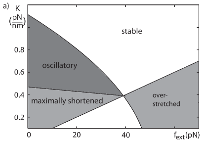
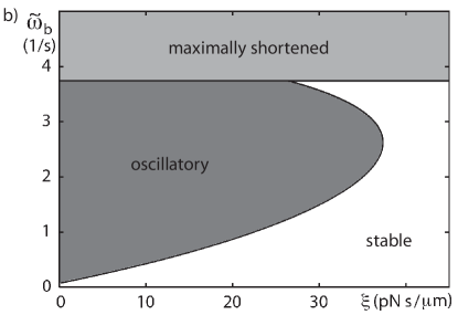
Figure 3 presents the regions of stability of the stationary state for different cuts through the parameter space. In Fig. 3a, the strength of the external force and of the elastic element are varied. For sufficiently small external forces and stiffness , the motors maximally shorten the element. As the stiffness is increased, the system starts to oscillate spontaneously. Upon a further increase, an inverse Hopf-bifurcation occurs and the stationary state is stable. Eventually, in the limit of large , the system will be forced to assume a length close to the rest length . If instead the external force is increased, a region of stable physical stationary states is reached. Beyond a critical value of the external force, though, the system is over-stretched and behaves as a simple elastic element with stiffness as the motors cannot interact with the polar filament. Note, that since the elastic elements of a real sarcomere are non-linear, a change in will affect also the value of that we use in the model.
In Figure 3b, we present the phase diagram resulting from changes in the motor activity and in the viscosity of the surrounding fluid. The latter influences the value of the effective friction constant . Changes in the motor activity affect several parameters. An important parameter is the binding rate of individual motors. The diagram shows that a decrease of the effective friction constant can induce oscillatory behavior. For sufficiently low values of , an increase of can first lead to an instability of the stationary state, while for too large values it is stable. This is reminiscent of the behavior predicted for spindle oscillations by a similar model [12], and for which there is experimental evidence [32]. Note, that due to the mechanism studied in Ref. [29, 30], changes in also affect the value of .
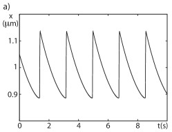
An example of an oscillation of a half-sarcomere is shown in Fig. 4a. It shows the characteristic saw-tooth shape which is observed experimentally: a slow contraction of the element is followed by a rapid expansion. As the motors shorten the element, the elastic force increases and therefore the force on the motors. This in turn increases the unbinding rate of motors. As a few motors detach from the filament, the remaining motors experience an even higher force, such that an avalanche of motor unbinding events occurs. The elastic element stretches the linker again and the motors rebind, the cycle can repeat.
3.2 A chain of half-sarcomeres
We now consider a chain of half-sarcomeres as studied in the previous section. It will be shown that the strong coupling between half-sarcomeres in a chain leads to traveling wave solutions that share essential features with waves observed experimentally in muscle fibers.
Consider a chain of half-sarcomeres, where the right end of a half-sarcomere is simultaneously the left end of the subsequent element. The right end of half-sarcomere in the chain is at position , the left end of the first-sarcomere is fixed at . Force balance of the half-sarcomere ends yields:
| (12) | |||||
| (13) | |||||
| (14) |
with . Here, , where and , denotes the friction force in the th half-sarcomere. The forces and are, respectively, the elastic and the motor force of half-sarcomere . The expressions for and are identical to those of an individual half-sarcomere. The dynamic equations for the extension and the fraction of bound motors in half-sarcomere are obtained from Eqs. (9) and (10), respectively, where , , and are replaced by , and .
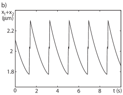
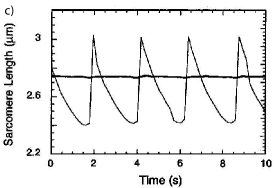
For the parameters given in A, a chain of half-sarcomeres, i.e., sarcomere, the asymptotic dynamic state is presented in Fig. 4b and compares nicely to experimental observations [17], see Fig. 4c. While a half-sarcomer essentially only shows two states, a stationary and an oscillatory, the dynamics of a sarcomere is richer. Oscillations of different symmetry classes can be identified as is reported in Ref. [33] where hydrodynamic interactions between half-sarcomeres have been included. A detailed study of the bifurcation diagram of a sarcomere will be presented elsewhere.
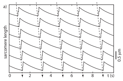
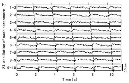
In Figure 5 a spontaneous wave along a chain of 20 half-sarcomeres is presented for the parameter values given in A and compared to an experimentally observed wave in a cardiac muscle fiber [20]. In both cases a relaxation wave travels from the left to the right. The temporal period of individual sarcomeres is the similar in the simulation and the experiment, the corresponding oscillation amplitude somewhat larger in the theory. The relative phase shift between the oscillations in adjacent sarcomeres differs by less than 10% between theory and experiment.
Note, that experimentally, cases are also observed, where the relaxation wave starts at the right of the fiber rather than at the left, leading to a wave traveling from right to left. In still other cases, the wave is initiated at some point along the fiber, traveling to the right and to the left starting form that point. The same is observed in numerical solutions of a chain of half-sarcomeres: depending on the initial conditions the wave can start anywhere along the chain. In addition to regular waves, for other parameter values we also find states where individual sarcomeres oscillate, but no coherent relaxation wave is formed.
3.3 The continuum limit
In order to get further insight into the spontaneous waves and to compare the model presented in this section with the phenomenological approach presented in Sect. 2, we now study the continuum limit of an infinite chain. It will be shown, that in this limit and neglecting the binding dynamics of the motors, the hydrodynamic description is obtained.
In the continuum limit, we will neglect all non-linear terms. Thus we first linearize Eqs. (9), (10) and (13) with respect to the stationary state (. In the linearized Eq. (13), we then approximate the differences , where is now the coordinate along the chain. The gradients in are just the strain in the chain and can be linked to the density along the chain. Consider a piece of length of the chain. On one hand, changing the density from its stationary value to changes the mass in this piece as . On the other hand, the change in density can be linked to a change in the distance between the particles (the end-points of the half-sarcomeres) according to , where and are the end points of the piece. Since the piece was arbitrarily chosen, we find .
Eliminating the equation for , we then arrive at
| (15) | |||||
| (16) |
Here, the constants are related to the microscopic parameters via
| (17) | |||||
| (18) | |||||
| (19) | |||||
| (20) | |||||
| (21) |
In the case of a stationary fraction of bound motors, Eq. (15) has the same form as the hydrodynamic equation of motion (8) and relations (17) and (18) relate the phenomenological parameters to microscopic parameters. We again find, that the dynamics of the fraction of bound motors, which clearly is not a hydrodynamic mode, is essential for obtaining waves along the a chain of half-sarcomeres. A linear stability of the homogenous stationary state of Eqs. (15) and (16) yields the same necessary condition as above for oscillatory solutions, as found above.
4 Discussion
In the preceding sections, we have presented theoretical descriptions of the dynamics of muscle fibers. Using a hydrodynamic approach where the system is described as a one-dimensional complex fluid close to thermodynamic equilibrium, we obtained a bound on the system’s activity to obtain contraction. Based upon a microscopic model of half-sarcomeres, we found oscillatory states that correspond to traveling waves along the fiber. The essential ingredient underlying this dynamic behavior is contained in a force dependence of the binding-unbinding kinetics of myosin motors to actin filaments. Spontaneous oscillations of sarcomeres and contraction waves along muscle fibers are observed experimentally and have been studied intensively [13, 14, 15, 16, 17, 18, 19, 20]. In the following paragraphs, we will compare experimental findings to our theoretical results.
First of all, sarcomeres have been observed to spontaneously oscillate under constant non-physiological conditions [13]. They consist of a slow contraction and a fast expansion phase, leading to a saw-tooth pattern of the sarcomere extension vs. time curve. It was shown experimentally that the oscillations are not induced by resonances with an external load, leading to the conjecture that spontaneous oscillations should be possible also in the absence of an external load [19]. Our (half-)sarcomere model generates behavior that is certainly consistent with these results and conclusions.
By choosing parameter values that are compatible with the values known from muscle and muscle myosin, the oscillatory solutions we find match the experimentally observed semi-quantitatively. Parameters could always be fitted such that the experimentally observed period and amplitude of the oscillations match exactly. Note, however, that these differ for different kinds of muscle. We therefore chose one typical set of parameters as explained in A without aiming at quantitatively matching a particular experiment.
Parameter values have been systematically varied in experiments. Unfortunately, variations in the chemical composition of the buffer solution, are not readily translated into changes of the parameter values we employ in our model. This holds in particular for the activity of the motors. In the buffers studied experimentally, motors are always only partially activated. The degree of the activation, however, is not assessed directly. Still, a few comparisons can be made. First of all, the oscillation frequency does not depend on the applied external force [17]. The same holds for the critical frequency at the onset of the oscillatory instability in the model. Furthermore, it has been shown that the oscillatory regime is an intermediate state between relaxation and contraction [13, 15] that can be continuously connected by changing the degree of motor activity [18]. Changes in the degree of motor activity, can in our model for example be described by increasing the binding rate of motors to the polar filament. In that case, we also observe a transition from a relaxed state, to an oscillatory state and then a maximally contracted state, see Fig. 3b.
Experimentally, spontaneous oscillations are observed only if a moderate external force is applied [14]. At first sight, this might be incompatible with the phase diagram presented in Fig. 3a. Indeed, if only the external force is varied, then the system can at best be driven form an oscillating state to a non-oscillating one. However, one has to keep in mind, that we have made the assumption of linear elastic elements. In a sarcomere, though, the elasticity is non-linear. While for the oscillations it is not essential to keep the non-linearity, it implies that with the application of an external forces also the value of the effective stiffness changes (it might either increase or decrease). By describing a curvilinear path in the (,)-plane when changing , the experimental observation and the theoretical results can be compatible. Furthermore, changes in the external force might affect other model parameters, for example, through the mechanism of stretch activation.
As already mentioned in the previous section, all the kinds of traveling waves observed in experiments have their counter-part in solutions to the chain equations. In particular, the propagation speed in terms of relative phase shifts between adjacent sarcomeres compares nicely.
In our analysis, we have neglected the effects of noise in our system. It has been shown in Ref. [12], where a similar approach was followed to describe oscillations of mitotic spindles during asymmetric cell division, that the mean-field analysis faithfully reproduced the features of the stochastic system. The same can be expected to hold in the present case.
In summary, we have presented a first semi-quantitative analysis of spontaneous oscillations of muscle fibers. It will now be interesting to design experiments that could specifically change parameters of the model and thereby test the importance of a force-dependent binding-unbinding kinetics of molecular motors for the observed oscillations. Due to the wide-spread appearance of motor oscillations, a quantitative combined experimental and theoretical study will likely help us to understand various cellular processes.
Appendix A Parameters
In this appendix, we discuss the parameter values that we have used in our numerical solutions of the dynamic equations presented in Sect. 3.1.1. As the parameter values differ for the various kinds of muscle used in experiments, we will present here typical values rather than trying to argue why a specific value has to be chosen for describing a particular experiment.
Let us start by geometric considerations. A typical rest length of an inactive sarcomere is m [7], so we take m, where is the rest length of the elastic element of a half-sarcomere. Typical lengths of actin filaments are m and m for myosin filaments, the latter consisting of about 300 Myosin-II molecules [7]. Correspondingly, the average distance between two adjacent motors on a myosin filament is nm.
In a muscle fiber, the approximately 1000 myosin filaments are arranged in a hexagonal lattice interdigitating with a hexagonal lattice of actin filaments. In a slice of thickness perpendicular to the orientation of the filaments, however, only a fraction of the motors can actually bind to an actin filament. This is because myosin binding sites are evenly spread on an actin filament every 37nm. Assuming that a motor head can bind within 4nm around its equilibrium position with respect to the motor filament, we arrive at about 100 motors that actually can bind in a slice of thickness .
As mentioned in Sect. 3.1.1, an ensemble of non-processive Myosin-II can be considered as one effectively processive motor. The time an individual motor spends bound to an actin filament is about 5ms [6]. As in the experiments motors are only partially activated [13, 18], we choose here ms. The binding rate can then be inferred from the duty ratio , which gives the fraction of time a motor is attached to a filament during a whole cycle. We choose which is in the middle of the predicted range [6]. From the values of individual motors, the parameters characterizing the effective motor can be inferred [31]. For the effective motor, we furthermore choose a stall force pN and a load-free velocity m/s. These values are lower than what might be obtained from single molecule experiments and again account for the only partial activation of motors in the experiments.
The elastic components entering our model are experimentally hard to assess. Single molecule experiments with Myosin-II suggest a stiffness of the linker of the head to the motor filament of the order of pN/nm [6, 34]. We are not aware of measurements of . Contributions come from titin molecules [35] the Z-discs and other elements. We choose pN/nm. Similarly, the microscopic length scale is unknown. It must be of molecular dimensions and we choose nm. Experiments are carried out at room temperature, such that pN nm.
Finally, friction in muscle fibers results from protein-protein friction as well as from hydrodynamic friction. Their effects are lumped into the parameter . Assuming a viscosity of ten times the viscosity of water Pa s, we use for the effective friction coefficient pN sm.
References
References
- [1] K. Kruse and F. Jülicher, Curr. Opin. Cell Biol. 17, 20 (2005).
- [2] A. Goldbeter, Nature 420, 238 (2002).
- [3] L. Rothfield, A. Taghbalout, and Y.L. Shih, Nat. Rev. Microbiol. 3, 959 (2006).
- [4] P. Martin and A.J. Hudspeth, Proc. Natl. Acad. Sci. USA 96, 14306 (1999).
- [5] D. Bray, Cell Movements 2nd ed. (Garland, New York, 2001).
- [6] J. Howard, Mechanics of Motor Proteins and the Cytoskeleton (Sinauer Associates, Inc., Sunderland, 2001).
- [7] B. Alberts et al., in Molecular Biology of the Cell, (Garland Publishing, New York, 2002).
- [8] F. Jülicher and J. Prost, Phys. Rev. Lett. 78, 4510 (1997).
- [9] C.J. Brokaw, Proc. Natl. Acad. Sci. USA 72, 3102 (1975).
- [10] S. Camalet, F. Jülicher, and J. Prost, Phys. Rev. Lett. 82, 1590 (1999).
- [11] S. Camalet and F. Jülicher, N. J. Phys. 2, 1 (2000).
- [12] S. Grill, K. Kruse, and F. Jülicher, Phys. Rev. Lett. 94, 108104 (2005).
- [13] N. Okamura and S. Ishiwata, J. Muscle Res. Cell Motil. 9, 111 (1988).
- [14] T. Anazawa, K. Yasuda, and S. Ishiwata, Biophys. J. 61 1099 (1992).
- [15] S. Ishiwata et al., Adv. Exp. Med. Biol. 332 545 (1993).
- [16] S. Ishiwata and K. Yasuda, Phase Transitions 45, 105 (1993).
- [17] K. Yasuda, Y. Shindo, and S. Ishiwata, Biophys. J. 70 1823 (1996).
- [18] N. Fukuda, H. Fujita, T.Fujita, and S. Ishiwata, Eur. J. Physiol. 433, 1 (1996).
- [19] H. Fujita and S. Ishiwata, Biophys. J. 75, 1439 (1998).
- [20] D. Sasaki, H. Fujita, N. Fukuda, S. Kurihara, and S. Ishiwata, J. Muscle Res. Cell Motil. 26 (2005).
- [21] A. Vilfan and T.A.J. Duke, Phys. Rev. Lett. 91, 114101 (2003).
- [22] D.A. Smith and D.G. Stephenson, J. Muscle Res. Cell Motil. 15, 369 (1994).
- [23] K. Kruse, A. Zumdieck, and F. Jülicher, Europhys. Lett. 64, 716 (2003).
- [24] K. Kruse, J.F. Joanny, F. Jülicher, J. Prost, and K. Sekimoto, Phys. Rev. Lett. 92, 078101 (2004).
- [25] K. Kruse, J.F. Joanny, F. Jülicher, J. Prost, and K. Sekimoto, Eur. Phys. J. E 16, 5 (2005).
- [26] A. Zumdieck, M.C. Lagomarsino, C. Tanase, K. Kruse, B. Mulder, M. Dogterom, and F. Jülicher, Phys. Rev. Lett. 95, 258103 (2005).
- [27] K. Kruse, J.F. Joanny, F. Jülicher, and J. Prost, Phys. Biol. 3, 130 (2006).
- [28] S.R. de Groot and P. Mazur, Non-equilibrium Thermodynamics, (Dover, New York, 1984).
- [29] K. Tawada and K. Sekimoto, J. Theor. Biol. 150, 193 (1991).
- [30] K. Tawada and K. Sekimoto, Biophys. J. 59, 343 (1991).
- [31] S. Klumpp and R. Lipowsky, Proc. Natl. Acad. Sci. USA 59, 17284 (2005).
- [32] J. Pecreaux, J.C. Röper, K. Kruse, F. Jülicher, A.A. Hyman, S.W. Grill, and J. Howard, Curr. Biol. 16, 2111 (2006).
- [33] S. Günther and K. Kruse, submitted (2007).
- [34] I. Schwaiger, C. Sattler, D. Hostetter, and M. Rief, Nat. Mat. 1, 232 (2002).
- [35] L. Tskhovrebova and J. Trinick, Nat. Rev. Mol. Cell Biol. 4 679 (2003).