Location- and observation time-dependent quantum-tunneling

Abstract

We investigate quantum tunneling in a translation invariant chain of particles. The particles interact harmonically with their nearest neighbors, except for one bond, which is anharmonic. It is described by a symmetric double well potential. In the first step, we show how the anharmonic coordinate can be separated from the normal modes. This yields a Lagrangian which has been used to study quantum dissipation. Elimination of the normal modes leads to a nonlocal action of Caldeira-Leggett type. If the anharmonic bond defect is in the bulk, one arrives at Ohmic damping, i.e. there is a transition of a delocalized bond state to a localized one if the elastic constant exceeds a critical value $C_{crit}$. The latter depends on the masses of the bond defect. Superohmic damping occurs if the bond defect is in the site $M$ at a finite distance from one of the chain ends. If the observation time $T$ is smaller than a characteristic time $\tau_{M}\sim M$, depending on the location $M$ of the defect, the behavior is similar to the bulk situation. However, for $T\gg\tau_{M}$ tunneling is never suppressed.

I INTRODUCTION

The influence of environmental degrees of freedom (DOF) on quantum phenomena, like e.g. tunneling, has been of great interest during the last decades 1 ; 2 ; 3 . A significant progress came from the investigation of a more or less phenomenological model where a particle in a one-dimensional potential $V(q)$ or a free particle is coupled to a bath of harmonic oscillators with the spectral density $J(\omega)$. The quantum dissipation generated by the bath depends qualitatively on the low frequency behavior of $J(\omega)$ 1 ; 2 ; 3 . A particular interesting case is Ohmic damping, when $J(\omega)\sim\omega$ for low enough frequencies. In that case and for a symmetric double well potential, the particle at zero temperature undergoes a transition from a delocalized state to a localized one if the coupling constant between the particle and bath exceeds a critical value 4 . An interesting observation has been made by Caldeira and Leggett 5 . The exponent of the exponential factor for the tunneling probability is multiplied by $\eta$, the phenomenological friction coefficient of the corresponding classical dynamics. This relationship between classical and quantum dissipation has been deepened and generalized by Leggett 6 for an arbitrary linear coupling between the particle and bath coordinates.

Let $\tilde{q}(\omega)$ be the Fourier transform of the classical particle trajectory $q(t)$ and

$$\widetilde{K}_{0}(\omega)\tilde{q}(\omega)+\frac{\widetilde{\partial V}}{\partial q}(\omega)=0$$ (1)

the transformed classical equation of motion, where $\widetilde{K}_{0}(\omega)$ contains the dissipative influence of the bath. Then the reduced Euclidean particle propagator $G_{E}(q^{\prime},T|q,0)$ (where the harmonic DOF have been eliminated) can be represented by a path integral in the imaginary time $t=-i\tau$ 7

$$G_{E}(q^{\prime},T|q,0)=\int\limits_{q(0)=q\atop q(T)=q^{\prime}}\mathcal{D}[q(\tau)]e^{-\frac{1}{\hbar}S[q(\tau)]}\qquad.$$ (2)

The action

$$S[q(\tau)]=S_{0}[q(\tau)]+S_{nonlocal}[q(\tau)]$$ (3a)

contains the local

$$S_{0}[q(\tau)]=\int\limits_{0}^{T}d\tau\,\left[\frac{M_{p}}{2}\dot{q}(\tau)^{2}+V(q(\tau))+\frac{\mu}{2}q(\tau)^{2}\right]$$ (3b)

and the nonlocal part

$$S_{nonlocal}[q(\tau)]=-\int\limits_{0}^{T}\,d\tau\int\limits_{0}^{\tau}\,d\tau^{\prime}\,K(\tau-\tau^{\prime})q(\tau)q(\tau^{\prime})=-\frac{1}{2\pi}\frac{1}{2}\int d\omega\,\widetilde{K}(\omega)|\tilde{q}(\omega)|^{2}.$$ (3c)

The second equality holds for $T\rightarrow\infty$. $\widetilde{K}(\omega)$ is the Fourier transform of the integral kernel $K(\tau)$ and it is related to $\widetilde{K}_{0}(\omega)$ by $\widetilde{K}(\omega)=\frac{1}{2}\widetilde{K}_{0}(-i|\omega|)$. If the Euclidean Lagrangian of the particle-bath system is

$$L=L_{0}+L_{1}\quad,\qquad L_{1}=L_{bath}+L_{int}$$ (4a)

with

$$L_{0}(q,\dot{q})=\frac{1}{2}M_{p}\dot{q}^{2}+V(q),$$ (4b)

and

$$L_{1}(q,\underline{x};\dot{q},\underline{\dot{x}})=\frac{1}{2}\sum_{\alpha=1}^{N}m_{\alpha}\left[\dot{x}_{\alpha}^{2}+\omega_{\alpha}^{2}\left(x_{\alpha}-\frac{c_{\alpha}}{m_{\alpha}\omega_{\alpha}^{2}}q\right)^{2}\right]$$ (4c)

then1 ; 2 ; 3

$$\mu=\frac{2}{\pi}\int\limits_{0}^{\infty}d\omega\,\frac{J(\omega)}{\omega}$$ (5a)

and

$$K(\tau)=\frac{1}{\pi}\int\limits_{0}^{\infty}d\omega\,J(\omega)\frac{\cosh(\omega(\frac{T}{2}-|\tau|))}{\sinh(\omega\frac{T}{2})}$$ (5b)

with the spectral density

$$J(\omega)=\frac{\pi}{2}\sum_{\alpha=1}^{N}\frac{c_{\alpha}^{2}}{m_{\alpha}\omega_{\alpha}}\delta(\omega-\omega_{\alpha})\qquad.$$ (5c)

For a finite $T$ the kernel $K(\tau)$ and the paths $q(\tau)$ can be periodically continued. Then the Fourier series for $K(\tau)$ is given by the Fourier coefficients 3

$$K_{n}=\frac{1}{T}\sum_{\alpha}\frac{c_{\alpha}^{2}}{m_{\alpha}}\frac{1}{\nu_{n}^{2}+\omega_{\alpha}^{2}}$$ (6)

with $\nu_{n}=(2\pi/T)n,\quad n=0,\pm 1,\pm 2,...$. Here $M_{p}$ and $\{m_{\alpha}\}$ are the masses of the particle and harmonic oscillators, respectively. $\{\omega_{\alpha}\}$ are the oscillator frequencies and $\{c_{\alpha}\}$ are the coupling constants between q and the coordinates of the oscillators $\{x_{\alpha}\}$. Note that $\{x_{\alpha}\}$ are not necessarily positions, but can represent normal mode coordinates of vibrations, etc.

In the following we will restrict ourselves to a system of $N$ particles whose potential energy $V(\vec{x}_{1},\ldots,\vec{x}_{N})$ includes harmonic and anharmonic interactions. Without an external field, $V$ must be translationally invariant. However, since the coordinates of Langrangian (4) are not specified, it is not necessarily invariant under translations. This has motivated Chudnovsky 8 to apply the Caldeira-Leggett approach to a system of two particles ($i=1,2$) with positions $x_{i}$ and masses $M_{i}$, coupled to oscillators with coordinates $x_{\alpha}$, frequencies $\omega_{\alpha}$ and masses $m_{\alpha},\alpha=1,\ldots,N$. The corresponding Euclidean Lagrangian is of the form

$$L=\frac{M_{1}}{2}\dot{x}_{1}^{2}+\frac{M_{2}}{2}\dot{x}_{2}^{2}+V(x_{1}-x_{2})+\frac{1}{2}\sum_{\alpha=1}^{N}m_{\alpha}\left[\dot{x}_{\alpha}^{2}+\omega_{\alpha}^{2}(x_{\alpha}-x_{2})^{2}\right]$$ (7)

with $V(x_{1}-x_{2})$ being the interaction energy between both particles. The coupling of particle $i=1$ to the oscillators is assumed to be zero. It is obvious that $L$ is translationally invariant under $x_{i}\longrightarrow x_{i}+a\,,\quad x_{\alpha}\longrightarrow x_{\alpha}+a$ provided that $\{x_{\alpha}\}$ are real space coordinates. Surprisingly the elimination of harmonic DOF does not lead for zero temperature to a nonlocal action of Caldeira-Leggett type (cf. Eqs. (3c), (5b),(6)). The Fourier coefficients of Chudnovsky’s kernel have the form

$$K_{n}^{c}=\frac{2}{T}\frac{M_{1}^{2}\nu_{n}^{2}}{M_{1}+M_{2}+\displaystyle\sum_{\alpha}\frac{m_{\alpha}\omega_{\alpha}^{2}}{\nu_{n}^{2}+\omega_{\alpha}^{2}}},$$ (8)

which differs qualitatively from the Caldeira-Leggett type result (6). However, for $M_{1}\rightarrow\infty$ one gets

$$K_{n}^{c}\rightarrow\frac{2}{T}(M_{1}-M_{2})\nu_{n}^{2}-\frac{1}{T}\sum_{\alpha}2m_{\alpha}\omega_{\alpha}^{2}\frac{\nu_{n}^{2}}{\nu_{n}^{2}+\omega_{\alpha}^{2}}$$ (9)

where the last term, up to the additional factor $-\nu_{n}^{2}$, corresponds to the second order time derivative of the kernel, identical to $K_{n}$ from Eq. (6), if one chooses $c_{\alpha}^{c}=\sqrt{2}m_{\alpha}\omega_{\alpha}$8 .

Then the question arises: Does a translationally invariant model in general lead to a nonlocal action, which is not of Caldeira-Leggett type? This is one of the main points we want to investigate among others in our paper. It will be done for a microscopic(within a Born-Oppenheimer approximation), explicitly translationally invariant lattice model with a defect which cannot diffuse. We will show how the normal mode coordinates for the harmonic DOF can exactly be separated from the anharmonic ones. This leads to a Lagrangian of the form of Eq. (4) with coupling constants $c_{\alpha}$, frequencies $\omega_{\alpha}$ and a spectral density determined by the microscopic model parameters. Such a microscopic justification of Lagrangian (4) has been presented for quantum diffusion 9 . There a particle diffusing through an elastic lattice is considered. If, however, that particle cannot diffuse and is an integral part of the lattice, e.g. an impurity which can tunnel only between two positions, one has to separate the center of mass (COM) and relative coordinates of all particles. For such a situation, Sethna 10 has estimated the coupling constants $c_{\alpha}$ by comparing the strain field of an elastic monopole of an impurity with the displacement for a longitudinal mode. But, as far as we know, there is no microscopic derivation available for the quantities $c_{\alpha}$, $\omega_{\alpha}$ and $J(\omega)$ for a non-diffusing impurity in a lattice. Besides such a microscopic derivation we will show that the quantum behavior of the defect is sensitive to its location.

The outline of our paper is as follows: Section II presents our model and outlines the main steps leading to Lagrangian (4). The implications for the quantum behavior will be discussed in the third section with a special emphasis on the role of defect location. A summary and conclusions are contained in the final section IV. Appendices A, B and C contain details on the separation of the harmonic and anharmonic DOF.

II Model

We consider an open chain of $N$ particles with masses $m_{n},\ n=1,\ldots,N$ and harmonic nearest neighbor interactions and one anharmonic bond representing a defect. This model could describe a linear macromolecule with an impurity. The classical Hamiltonian reads

$$H=\sum_{n=1}^{N}\frac{1}{2m_{n}}p_{n}^{2}+V(x_{1},...,x_{N})$$ (10a)

with the potential energy

$$V(x_{1},...,x_{N})=\frac{C}{2}\sum_{n=1\atop(\neq M)}^{N-1}(x_{n+1}-x_{n}-a)^{2}+V_{0}(x_{M+1}-x_{M})\qquad.$$ (10b)

in which $x_{n}$ is the position of $n$-th particle, $C$ is the elastic constant of the harmonic nearest neighbor interaction, $a$ is the equilibrium length of the harmonic bonds and $V_{0}(x_{M+1}-x_{M})$ is the energy of the anharmonic bond defect located between the sites $M$ and $M+1$. The potential energy $V$ is explicitly translationnally invariant. Several ways exist to separate the harmonic and anharmonic DOF, which finally lead to the Langrangian (4) (see Appendices B and C). One (see Appendix B), which is also applicable in higher dimensions, is to introduce the COM

$$X_{d}=\frac{1}{m_{M}+m_{M+1}}\left(m_{M}x_{M}+m_{M+1}x_{M+1}\right)$$ (11a)

and relative coordinates of the bond defect

$$q_{M}=x_{M+1}-x_{M}\qquad.$$ (11b)

Then, $x_{1},\ldots,x_{M-1},X_{d},x_{M+1},\ldots,x_{N}$ are harmonic coordinates. Their kinetic and potential energy can be diagonalized by introducing normal coordinates. $q_{M}$ is linearly coupled to these coordinates. As a result, one obtains the Lagrangian (4). Here we will choose a different approach applicable to 1d systems, which, however, leads to the same Lagrangian. Let

$$X_{c}=\frac{1}{M_{c}}\sum_{n=1}^{N}m_{n}x_{n}\,,\quad M_{c}=\sum_{n=1}^{N}m_{n}$$ (12a)

be the COM of all the particles and

$$q_{i}=x_{i+1}-x_{i}-a_{i}\,,\quad i=1,...,N-1,$$

$$a_{M}=0\,,\quad\mbox{and}\ a_{i}=a\,\quad\mbox{otherwise,}$$ (12b)

be the relative coordinates, respectively. Using notation $q_{0}=X_{c}$, Eq. (12a),(12b) has the form

$$q_{i}+a_{i}=\sum_{n=1}^{N}A_{in}x_{n}\,,\quad i=0,1,...,N-1\qquad.$$ (13a)

with

$$A_{in}=\frac{m_{n}}{M_{c}}\delta_{0,i}+(\delta_{i,n+1}-\delta_{i,n})(1-\delta_{0,i})$$

Let $\pi_{i}$ be the canonical conjugate momenta of $q_{i}$. It is easy to prove that Eq. (13a) implies

$$p_{n}=\sum_{i=0}^{N-1}A_{in}\pi_{i}\,,\quad n=1,...,N\qquad.$$ (13b)

Substituting $p_{n}$ into Eq. (13a) yields

$$H = \frac{1}{2M_{c}}\pi_{0}^{2}+\frac{1}{2}\sum_{i=1}^{N-1}\left(\frac{1}{m_{i}}+\frac{1}{m_{i+1}}\right)\pi_{i}^{2}-\sum_{i=1}^{N-2}\frac{1}{m_{i+1}}\pi_{i}\pi_{i+1}$$ (14)

$$+\frac{C}{2}\sum_{i=1\atop(i\neq M)}^{N-1}q_{i}^{2}+V_{0}(q_{M})\qquad.$$

Here the first term is the kinetic energy of COM, which will be dropped from now on. Note that the use of relative coordinates introduces a coupling between the momenta. In the next step, we perform the canonical transformation

$$\pi_{i}=\tilde{p}_{i}\,,\quad i=1,...,N-1;\,i\neq M,$$

$$\pi_{M}=\tilde{p}_{M}+\frac{1}{m_{M}+m_{M+1}}\left(m_{M+1}\tilde{p}_{M-1}+m_{M}\tilde{p}_{M+1}\right),$$ (15a)

$$q_{i}=\tilde{q}_{i}\,,\quad i=1,...,N-1;\,i\neq M\pm 1$$

$$q_{M-1}=\tilde{q}_{M-1}-\frac{m_{M+1}}{m_{M}+m_{M+1}}\tilde{q}_{M},$$ (15b)

$$q_{M+1}=\tilde{q}_{M+1}-\frac{m_{M}}{m_{M}+m_{M+1}}\tilde{q}_{M}\qquad.$$

This leads to

$$H=H_{d}+H_{harm}+H_{int}$$ (16a)

where

$$H_{d}=\frac{m_{M}+m_{M+1}}{2m_{M}m_{M+1}}\tilde{p}_{M}^{2}+V_{0}(\tilde{q}_{M})+\frac{C}{2}\frac{m_{M}^{2}+m_{M+1}^{2}}{(m_{M}+m_{M+1})^{2}}\tilde{q}_{M}^{2}$$ (16b)

is the defect Hamiltonian,

$$H_{harm}=\frac{1}{2}\sum_{i,j=1\atop(\neq M)}^{N-1}T_{ij}\tilde{p}_{i}\tilde{p}_{j}+\frac{C}{2}\sum_{i=1\atop(\neq M)}^{N-1}\tilde{q}_{i}^{2}\qquad.$$ (16c)

is the harmonic part of the Hamiltonian and

$$H_{int}=-C\frac{m_{M+1}\tilde{q}_{M-1}+m_{M}\tilde{q}_{M+1}}{m_{M}+m_{M+1}}\tilde{q}_{M}$$ (16d)

is the coupling between the two.

The matrix $\textbf{T}=(T_{ij})$ in (16c) depends on the masses $m_{i}$ (see Appendix A). Let $\textbf{e}^{(\alpha)}=(e_{1}^{(\alpha)},\ldots,e_{M-1}^{(\alpha)},e_{M+1}^{(\alpha)},\ldots,e^{(\alpha)}_{N-1})^{t}$ and $\lambda_{\alpha}$ be the normalized eigenvectors and eigenvalues of T, respectively, and

$$\mathbf{S}=(\mathbf{e}^{(1)},\ldots,\mathbf{e}^{(N-2)})$$

be the orthogonal matrix, which diagonalizes T, i.e.

$$\mathbf{S^{-1}TS}=\mathbf{\Lambda}\,,\quad\Lambda_{\alpha\beta}=\lambda_{\alpha}\delta_{\alpha\beta}.$$ (17)

Then we can introduce the normal coordinates

$$x_{\alpha}=\sum_{i=1\atop(\neq M)}^{N-1}S_{\alpha i}\tilde{q}_{i}\,,\quad p_{\alpha}=\sum_{i=1\atop(\neq M)}^{N-1}S_{\alpha i}\tilde{p}_{i}$$ (18)

for $\alpha=1,2,...,N-2$ such that $H_{harm}$ becomes diagonal

$$H_{harm}=\frac{1}{2}\sum_{\alpha=1}^{N-2}\left[\lambda_{\alpha}p_{\alpha}^{2}+Cx_{\alpha}^{2}\right]\qquad.$$ (19a)

The interaction term takes the form

$$H_{int}=-\sum_{\alpha=1}^{N-2}c_{\alpha}x_{\alpha}q_{M}\qquad.$$ (19b)

The $M$ dependent coupling constants are given by

$$c_{\alpha}=C\frac{1}{m_{M}+m_{M+1}}\left[m_{M+1}e^{(\alpha)}_{M-1}+m_{M}e^{(\alpha)}_{M+1}\right]\qquad.$$ (20)

The final step is the Legendre transformation of $H$, which leads to the Euclidean Lagrangian

$$L=L_{d}+L_{1}\,,\quad L_{1}=L_{harm}+L_{int}$$ (21a)

where

$$L_{d}=\frac{1}{2}\widetilde{m}\dot{q}_{M}^{2}+V_{0}(q_{M}),$$ (21b)

and

$$L_{1}=\frac{1}{2}\sum_{\alpha=1}^{N-2}m_{\alpha}\left[\dot{x}_{\alpha}^{2}+\omega_{\alpha}^{2}\left(x_{\alpha}-\frac{c_{\alpha}}{m_{\alpha}\omega_{\alpha}^{2}}q_{M}\right)^{2}\right]\qquad.$$ (21c)

Here we have used the equality $\tilde{q}_{M}=q_{M}$ (cf. Eq. (15b)) and

$$\sum_{\alpha=1}^{N-2}\frac{c_{\alpha}^{2}}{m_{\alpha}\omega_{\alpha}^{2}}=C\frac{m_{M}^{2}+m_{M+1}^{2}}{(m_{M}+m_{M+1})^{2}}\,,$$ (22)

which follows from the completeness of the set $\textbf{e}^{(\alpha)}$ of eigenvectors and $1/(m_{\alpha}\omega_{\alpha}^{2})=1/C$ (see below). Eq. (22) allows us to include the counterterm $\frac{C}{2}\frac{m_{M}^{2}+m_{M+1}^{2}}{(m_{M}+m_{M+1})^{2}}q_{M}^{2}$ in Eq. (16b) into $L_{1}$. This counterterm, the role of which has been discussed by Caldeira and Leggett 11 , results from the canonical transformation, Eq. (15a), (15b). This transformation eliminates the coupling between the momenta of the harmonic DOF and that of the defect and generates coupling between the normal mode coordinates $\{x_{\alpha}\}$ and the corresponding defect variable $q_{M}$ (cf. Eq. (16d)). Due to the disappearance of the counterterm, there is no frequency renormalization for the bond defect3 . The Lagrangian (21) is identical to that of Eq. (4). The masses $m_{\alpha}$ and frequencies $\omega_{\alpha}$ follow from

$$m_{\alpha}=\frac{1}{\lambda_{\alpha}}\,,\quad\omega_{\alpha}=(C\lambda_{\alpha})^{\frac{1}{2}}$$ (23a)

and the reduced defect mass $\tilde{m}$ is given by

$$\widetilde{m}=\frac{m_{M}m_{M+1}}{m_{M}+m_{M+1}}\qquad\qquad.$$ (23b)

Note that these results are exact for one dimensional systems. It can be shown that for an arbitrary impurity in a two- or three-dimensional system the Langrangian (21) can be derived within a kind of harmonic approximation 12 .

III QUANTUM TUNNELING

In this section we will investigate the zero temperature quantum behavior of the anharmonic bond defect embedded in the harmonic chain as shown in Fig. 1.

Figure 1: Two degenerate classical ground states of the open chain with $N$ particles. The masses $m_{n}$, $n\neq M,M+1$ are chosen to be equal. $a$ is the equilibrium length of the harmonic bonds and $a_{s},a_{l}$ the two degenerate equilibrium lengths of the anharmonic bond.

We will assume that $V_{0}(q_{M})$ is a symmetric double-well potential with degenerate minima at $q^{-}_{M}=a_{s}>0$ and $q_{M}^{+}=a_{\ell}>a_{s}$. Then the classical ground state of $V(x_{1},\ldots,x_{N})$ (cf. Eq. 10b) is twofold degenerate (see Fig.1). Therefore the low-lying eigenstates form doublets. Neglecting the excited doublets at zero temperature is justified if the bare tunneling splitting of the ground state doublet is much less than the frequency of the upper phonon band edge $\omega_{0}$ (see Eq. (25a))1 . If the total number $N$ of particles in the chain is macroscopically large and the particle number $M$ is in the bulk of the chain, i.e. $M=\mathcal{O}(N)$, one might have expected a suppression of tunneling since the change from, e.g. $q^{-}_{M}=a_{s}$ to $q_{M}^{+}=a_{\ell}$, would require a translation of the macroscopic mass of the left and right harmonic parts of the chain. We will see that this naive expectation is not always correct.

On the other hand, if the defect is close to one of the free boundaries, i.e. either $M=\mathcal{O}(1)$ or $(N-M)=\mathcal{O}(1)$, only a finite mass $\sim M$ has to be translated. Consequently tunneling cannot be suppressed. This qualitative $M$-dependence should follow from that of the kernel $K(\tau)$, which itself results from the strong $M$-sensitivity of the spectral density $J(\omega)$. Subsection III.1 discusses this phenomenon. The limit $m_{M}\rightarrow\infty$ (or $m_{M+1}\rightarrow\infty$), motivated by the conclusions drawn in Ref. 8 , will be discussed in Subsection III.2.

III.1 Location-dependent quantum tunneling

As we will see in Subsection III.2 the form of the nonlocal action Eq. (3c) does not depend qualitatively on the masses $m_{n}$, even if one of the defect masses $m_{M}$ or $m_{M+1}$ becomes infinitely large. Therefore we will choose for convenience $m_{n}\equiv m$. Let us start with the situation where the bond defect is located within the bulk, i.e. $M=\mathcal{O}(N)$, so that

$$O<\lim\limits_{N\rightarrow\infty\atop M\rightarrow\infty}\frac{M}{N}=\xi<1.$$ (24)

One can prove that the tunneling phenomena do not depend on $\xi$ if it is different from 0 and 1. Therefore we choose $M=N/2$ and without loss of generality $N$ to be even. This choice and the assumption $m_{n}\equiv m$ allows us to determine the eigenfrequencies $\omega_{\alpha}$ and the eigenvectors $\mathbb{e}^{(\alpha)},\alpha=1,\ldots,N-2$ exactly for finite $N$. A calculation, whose technical details are presented in Appendix A, results in

$$\lambda_{\alpha}^{\pm}=\frac{4}{m}\sin^{2}\left(\frac{q_{\alpha}^{\pm}}{2}\right)\rightarrow\omega_{\alpha}=\omega_{0}\sin\left(\frac{q_{\alpha}}{2}\right)\,,\quad\omega_{0}=2\sqrt{\frac{C}{m}},$$ (25a)

$$e^{+(\alpha)}_{j}=\sqrt{\frac{2}{N-1}}\begin{cases}\sin(q^{+}_{\alpha}j)\quad&,\quad 1\leq j\leq M-1=\frac{N}{2}-1,\\ &\\ \sin(q^{+}_{\alpha}(j-1))\quad&,\quad M+1=\frac{N}{2}+1\leq j\leq N-1,\end{cases}$$

$$e^{-(\alpha)}_{j}=\sqrt{\frac{2}{N}}\sin(q^{-}_{\alpha}j)\,,\quad 1\leq j\leq N-1;\,j\neq M=\frac{N}{2},$$ (25b)

where

$$q_{\alpha}^{(\sigma)}=\begin{cases}\displaystyle\frac{\pi}{N-1}(2\alpha-1)\quad&,\quad\sigma=+,\\ &\\ \displaystyle\frac{\pi}{N}2\alpha\quad&,\quad\sigma=-\end{cases}$$ (25c)

for $\alpha=1,\ldots,N/2-1$. It is easy to see that $e_{j}^{+(\alpha)}$ are the symmetric eigenvalues with respect to $j\rightarrow N-j$ and $e_{j}^{-(\alpha)}$ are the antisymmetric ones. From this, $m_{n}\equiv m$ and Eq. (20) it is obvious that the bond defect does not couple to the antisymmetric vibrational modes, as may be expected from the symmetry of the problem. With these results we can calculate the spectral density. Making use of Eqs. (20), (23a), (25a), (25b) and (25c) we get from Eq. (5c) in the thermodynamic limit $N\rightarrow\infty$ that

$$J(\omega)=\frac{1}{2}C\omega_{0}\int\limits_{0}^{\pi}dq\,\cos^{2}\left(\frac{q}{2}\right)\sin\left(\frac{q}{2}\right)\delta\Bigl{(}\omega-\omega_{0}\sin\left(\frac{q}{2}\right)\Bigr{)}$$

$$=C\sqrt{1-\left(\frac{\omega}{\omega_{0}}\right)^{2}}\frac{\omega}{\omega_{0}}.$$ (26a)

In the limit $\omega\ll\omega_{0}$ we obviously have

$$J(\omega)\cong C\frac{\omega}{\omega_{0}}\,,$$ (26b)

which corresponds to the situation of Ohmic damping. The Ohmic damping results from two facts: First, the density of states $g(\omega)$ of the vibrational modes in a one-dimensional lattice is constant for $\omega\ll\omega_{0}$ and second the squared coupling constant involves the factor $\sin^{2}(q_{\alpha}M)$ which, for $N\rightarrow\infty$, $M\rightarrow\infty$ with $M/N=\xi(\neq 0,1)$, oscillates faster and faster so that it can be replaced by 1/2. It is emphasized that the condition $M=\mathcal{O}(1)$, i.e. $\xi=0$ or 1, will change the shape of $J(\omega)$ qualitatively.

Now we can calculate the kernel $K(\tau)$. For $\omega_{0}T\gg 1$ and $|\omega_{0}(\frac{T}{2}-|\tau|)|\gg 1$ the fraction in Eq. (5b) can be well approximated by $\exp(-\omega_{0}|\tau|\sin\frac{q}{2})$. The influence of the oscillators on tunneling of $q_{M}$ is determined by the large $-\tau$ behavior, i.e. by the low frequency modes. Therefore, substituting $J(\omega)$ from Eq. (26b) into Eq. (5b) we find, of course, the well-known result for Ohmic damping 1 ; 2 ; 3

$$K(\tau)\cong\frac{1}{\pi}C\omega_{0}\frac{1}{(\omega_{0}\tau)^{2}}\,,\quad\omega_{0}\tau\gg 1.$$ (27)

As a consequence, there exists a critical elastic constant $C_{crit}$ so that the anharmonic bond can tunnel for $C<C_{crit}$, despite macroscopic masses have to be moved (see Figure 1). For $C>C_{crit}$ symmetry is broken. If the anharmonic bond is prepared in its ground state, e.g. $q_{m}^{-}=a_{s}$, it will remain there on average.

If, however, the bond defect is located close to one of the boundaries, so that either $M=\mathcal{O}(1)$ or $N-M=\mathcal{O}(1)$ ($\xi=$ 0 or 1 in (24)), the situation changes. Note that we perform first the thermodynamic limit $N\rightarrow\infty$. Then $M=\mathcal{O}(1)$ means that $M$ may equal $1,2,...,10^{6}$ or even a larger, but still finite number. For $m_{n}\equiv m$ one can easily show that

$$c_{\alpha}=\frac{1}{2}C\left(e^{(\alpha)}_{M-1}+e_{M+1}^{(\alpha)}\right)=C\mathcal{N}_{\alpha}\sin\left(q_{\alpha}M\right)$$ (28)

where $\mathcal{N}_{\alpha}$ is the normalization constant of $\{e_{n}^{(\alpha)}\}$ (see Appendix A). Replacing $\mathcal{N}_{\alpha}$ by its low frequency behavior $(2/N)^{1/2}$ and taking the limits $\omega_{0}T\gg 1$ and $|\omega_{0}(\frac{T}{2}-|\tau|)|\gg 1$ yields

$$K_{M}(\tau)\cong\frac{1}{2}C\omega_{0}\frac{1}{\pi}\int\limits_{0}^{\pi}dq\,q\sin^{2}(qM)e^{-\frac{1}{2}\omega_{0}|\tau|q}$$ (29)

for the kernel. In order to be consistent we also replaced $\omega(q)=\omega_{0}\sin(q/2)$ by its low frequency dispersion $\omega(q)\cong\frac{1}{2}\omega_{0}q$. The integrand of Eq. (29) involves two $q$-scales

$$q_{M}=\frac{1}{M}\quad\quad\mbox{and}\ \quad q_{\tau}=\frac{1}{\omega_{0}|\tau|}\quad.$$ (30)

Equating $q_{M}=q_{\tau}$ defines the timescale

$$\tau_{M}=\omega_{o}^{-1}M.$$ (31)

The physical meaning of $\tau_{M}$ is as follows: The path integral formalism 7 ; 13 allows one to investigate quantum tunneling by determining the instanton solutions, i.e. the solutions of the classical equation of motion for a double well potential in imaginary time. The width $\tau_{kink}$ of a single instanton is

$$\tau_{kink}=\left(\frac{m}{V^{\prime\prime}_{0}(q_{M}^{\pm})}\right)^{1/2}\quad.$$

If we assume that $V^{\prime\prime}_{0}(q_{M}^{\pm})\approx C$, the elastic constant of the harmonic bonds, then $\tau_{kink}\approx\omega_{0}^{-1}$ so that

$$\tau_{M}\approx M\tau_{kink}\quad.$$ (32)

The $\tau$-dependence of $K_{M}(\tau)$ is sensitive to whether $|\tau|/\tau_{kink}\gg M$ or vice versa. Let us start with the long time limit

• $|\tau|/\tau_{M}\gg 1$.

  Then it follows from Eqs. (30) and (31) that $q_{\tau}\ll q_{M}$. The major contribution to the integral in Eq. (29) comes from $q<q_{\tau}\ll q_{M}$. Therefore, we are allowed to replace $\sin^{2}(qM)=\sin^{2}(q/q_{M})$ by $(q/q_{M})^{2}=(qM)^{2}$, which leads to the spectral density $J(\omega)\sim\omega^{3}$ at low frequencies corresponding to superohmic damping. It implies that $K_{M}(\tau)\sim\tau^{-4}$. The precise result is

  $$K_{M}(\tau)\cong\frac{48}{\pi}C\omega_{0}\frac{1}{(\omega_{0}\tau)^{4}}M^{2}\,,\quad|\tau|\gg\tau_{M}\quad.$$ (33)

  

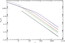
  Figure 2: $\tau$-dependence of $K_{M}(\tau)$ for $M=5,10,40$ and $160$ (from bottom to top) on a log-log representation. The dotted and dashed line, corresponds to $\tau^{-2}$ and $\tau^{-4}$, respectively. The crossover at $\tau\approx\tau_{M}$ from the $\tau^{-2}$ behavior to that of $\tau^{-4}$ can clearly be seen. The parameters have been chosen as follows: $T=10^{5},C=m=1\Rightarrow\omega_{0}=2$.

• A different situation takes place for $|\tau|/\tau_{M}\ll 1$.

  Then $q_{\tau}\gg q_{M}$ and the integral in Eq. (29) must be decomposed in two contributions $\int\limits_{0}^{q_{M}}dq\cdots+\int\limits^{\pi}_{q_{M}}dq\cdots$. The first integral yields a constant in the leading order in $\omega_{0}\tau/\tau_{M}=\omega_{0}\tau/M$. For the second one we are allowed to replace $\sin^{2}(qM)=\sin^{2}(q/q_{M})$ by $1/2$ since the main contribution comes from $q\approx q_{\tau}\gg q_{M}$ so that the function $\sin^{2}(qM)=\sin^{2}(q/q_{M})$ is oscillating fast between zero and one, whereas $\exp\left(-\frac{1}{2}\omega_{0}|\tau|q\right)=\exp\left(-\frac{1}{2}q/q_{\tau}\right)$ varies slowly. Accordingly $\tau\ll\tau_{M}$ corresponds to an ’effective’ spectral density $J(\omega)\approx\omega$, i.e. to Ohmic damping. It is straightforward to estimate both integrals. As the final result we obtain

  $$K_{M}(\tau)\cong\frac{1}{\pi}C\omega_{0}\Biggl{[}\frac{1}{8M^{2}}\biggl{(}1+\mathcal{O}\left(\frac{\omega_{0}|\tau|}{M}\right)\biggr{)}+\frac{1}{(\omega_{0}\tau)^{2}}\Biggr{]}$$ (34)

  for $\tau_{kink}\ll\tau\ll\tau_{M}\approx M\tau_{kink}$. Taking the limit $M\rightarrow\infty$ in Eq. (34) restores the result (27) for the kernel $K(\tau)$.

For $M=\mathcal{O}(1)$ or $N-M=\mathcal{O}(1)$, and $N\rightarrow\infty$ we obtain for $K_{M}(\tau)$ a crossover at $\tau_{M}$ from the power law   $\tau^{-2}$ for $\tau\ll\tau_{M}$ to $\tau^{-4}$ for $\tau\gg\tau_{M}$. Figure 2 illustrates this behavior for $K_{M}(\tau)$, calculated numerically. On the log-log plot of Figure 2 the crossover between both power laws can easily be observed.

This crossover is related to the $M$-dependence of the spectral density because the defect-phonon coupling constants $c_{\alpha}$ are $M$-dependent. If the ’observation time’ $T$ (which is the time $T$ in $G_{E}$ from Eq. (2)) is smaller than $\tau_{M}$ then $(\tau-\tau^{\prime})$ will be smaller than $\tau_{M}$, as well. Consequently the kernel $K_{M}(\tau-\tau^{\prime})$ entering the nonlocal action (Eq. (3c)) decays as $1/(\tau-\tau^{\prime})^{2}$. If, however, $T$ is larger than $\tau_{M}$ then it is possible that $(\tau-\tau^{\prime})$ becomes larger than $\tau_{M}$, as well. For those values of $(\tau-\tau^{\prime})$ the kernel $K_{M}$ decays as $1/(\tau-\tau^{\prime})^{4}$. This discussion reveals that the choice of the ’observation time’ $T$ allows to fix the ’large’-$\tau$ behavior of $K_{M}(\tau)$, where, of course, $\tau\leq T$. If $M$ is far away from the chain end the crossover time $\tau_{M}$ is correspondingly large. Increasing $M$ even more $\tau_{M}$ increases, too. Nevertheless, the ’observation time’ dependence still exists. It disappears for $M\rightarrow\infty$, only. We remind the reader that the limit $N\rightarrow\infty$ has to be taken first.

Now making use of the analogy 1 ; 3 ; 4 between the calculation of the action of a multi-instanton configuration interacting via $K_{M}(\tau-\tau^{\prime})$ and a one-dimensional Ising model with the coupling constants $J_{nm}\sim K_{M}(n-m)\sim|n-m|^{-k}$ we can conclude the following: If the ’observation time’ $T$ is smaller than $\tau_{M}$ then we have $K_{M}(\tau)\sim\tau^{-2}$, i.e. Ohmic damping. In that case the bond defect may tunnel for $C<C_{crit}(T)$, whereas symmetry becomes broken for $C>C_{crit}(T)$. Note, that this is not a sharp transition at $C_{crit}(T)$ since finite $T$ corresponds to a finite Ising chain which does not exhibit a sharp phase transition. What really happens when increasing the coupling constant $C$ is an increase of the correlation ’length’ $\xi(C)$. As soon as $\xi(C)$ equals the ’size’ $T$ of the Ising-chain a ’long range’ order occurs. However, if $T$ is much larger than $\tau_{M}\approx M\tau_{kink}$ we have $K_{M}(\tau)\sim\tau^{-4}$ and tunneling is never suppressed 1 ; 3 .

One might be puzzled by these conclusions since the transition for Ohmic damping to decoherence for $M=\mathcal{O}(N),N\rightarrow\infty$ occurs for large $T$, or to be more precise it becomes a sharp transition for $T=\infty$, only. As we already stressed above, the transition for $T<\tau_{M}$ is not sharp. The relevant phonons contributing to $K_{M}(\tau)$ have wavenumbers $q\approx q_{\tau}\sim q_{T}=\frac{1}{T}$. This makes the ’effective’ spectral density Ohmic. Mapping the situation for $M=\mathcal{O}(1)$ again onto the Ising chain of length $L$ results in the coupling constants $J_{nm}$ decaying like $J_{0}|n-m|^{-2}$ for $|n-m|<M$ and like $J_{0}|n-m|^{-4}$ for $|n-m|>M$. It is clear that there is no sharp phase transition for finite $L$. But if $L<M$, the coupling constants decay as $J_{0}|n-m|^{-2}$. For a fixed temperature $T$ (not to be confused with the ’observation time’ $T$) there will be no magnetic order ($\hat{=}$ coherent tunneling) for $J_{0}<J_{0,crit}(T)(\hat{=}\,C<C_{crit}(T))$. For $J_{0}>J_{0,crit}(T)(\hat{=}\,C>C_{crit}(T))$ a crossover to the ’long range order’ ($\hat{=}$ decoherent tunneling) takes place. Accordingly the quantum tunneling phenomenon is richer for $M=\mathcal{O}(1)$ than for $M=\mathcal{O}(N)$.

Actually we may think also in the real time $t$ terms that as long as only the phonons with relatively high frequencies $\omega\approx 1/t$ and hence short wave length such that $1/q<M$ participate in the interaction with the anharmonic defect, the latter does not ’feel’ that the chain is finite and behaves as in the Ohmic case. In the course of time the lower frequency phonons with higher wave length ’reach’ the end of the chain and a crossover to a superohmic behavior takes place.

III.2 Dependence on the masses of defect

In this subsection we will assume that

$$m_{n}=\begin{cases}m\quad&,\quad n\neq M,M+1,\\ M_{1}\quad&,\quad n=M,\\ M_{2}\quad&,\quad n=M+1.\end{cases}$$ (35)

For $M=\mathcal{O}(N)$ we may choose without loss of generality $M=N/2$ and $N$ being even. It is easy to prove that $e_{j}^{+(\alpha)}$ from Eq. (25b) remain eigenvectors of T with $q^{+}_{\alpha}$, $\alpha=1,2,\ldots,N/2-1$ given by Eq. (25c). The remaining $(N/2-1)$ eigenvectors are of the form

$$e^{-(\alpha)}_{j}=\mathcal{N}_{\alpha}^{-}\begin{cases}\sin(q^{-}_{\alpha}j)\quad&,\quad 1\leq j\leq\frac{N}{2}-1,\\ &\\ \sin(q^{-}_{\alpha}(N-j))\quad&,\quad\frac{N}{2}+1\leq j\leq N-1\quad.\end{cases}$$ (36a)

$q_{\alpha}^{-}$ is a solution of transcendental equation. Let us introduce the quantities $\beta_{i}=m/M_{i}$, $i=1,2$ and $\delta=\beta_{1}\beta_{2}/(\beta_{1}+\beta_{2})$. The limit $M_{1}\rightarrow\infty$ (or $M_{2}\rightarrow\infty)$ implies $\delta\rightarrow 0$. Since the results in 8 motivate us to study, e.g. $M_{2}\rightarrow\infty$, we find

$$q_{\alpha}^{-}=q_{\alpha}^{+}+\frac{1}{N-1}\frac{2\delta}{\tan(\frac{q^{+}_{\sigma}}{2})}+\mathcal{O}(\delta^{2})$$ (36b)

in the limit $\delta\rightarrow 0$. Substituting Eqs. (36a), (36b) into Eq. (20) yields

$$c_{\alpha}^{-}\cong c_{\alpha}^{+}\quad.$$

in the leading order in $\delta$. As a result $J(\omega)$ and therefore $K(\tau)$, too, are doubled as compared to the case of $M_{i}=m$, i.e. we get

$$K(\tau)\cong\frac{2}{\pi}C\omega_{0}\frac{1}{(\omega_{0}\tau)^{2}}\quad.$$ (37)

for $M_{2}\to\infty$.

The only essential result of changing $M_{2}$ from $m$ to infinity is that the critical elastic constant increases by a factor of two.

IV Summary and Conclusions

For a translationally invariant chain with one anharmonic bond and otherwise harmonic nearest neighbor interactions, we have shown exactly how the anharmonic degree of freedom can be separated from the harmonic ones in their normal mode representation. As a result, we have obtained Lagrangian (21), which is of the form of Lagrangian (4). Note, that this result can also be obtained for a three-dimensional system within the Born-Oppenheimer approximation starting with an arbitrary translationally invariant potential $V(\vec{x}_{1},\ldots,\vec{x}_{N})$ for a $N$-particle system 12 . Since the Caldeira-Leggett type nonlocal action 1 ; 2 ; 3 is based on the form (4) (or (21)) of the Lagrangian it is not the translation invariance and therefore not the conservation of momentum, which can lead to a different type of nonlocal action. The discrepancy between our results and those of Ref. 8 may have the following origin. Since the harmonic part of Lagrangian (7) is diagonal in $x_{\alpha}$, the harmonic variables $x_{\alpha}$ are already normal mode coordinates. In that case a translation of the full system only changes the Goldstone mode amplitude, let us say $x_{0}$, but leaves all the other normal mode coordinates unchanged, i.e. $x_{\alpha}\rightarrow x_{\alpha}$, $\alpha\neq 0$ for any translation. If $x_{1}$ and $x_{2}$ in Eq. (7) are real space coordinates then the coupling term $(x_{\alpha}-x_{2})^{2}$ is not translationally invariant for $\alpha\neq 0$.

Our model has allowed us to calculate explicitly, e.g. for $m_{n}=m$ and $M=N/2$ the coupling constants $c_{\alpha}$, the eigenfrequencies $\omega_{\alpha}$ and the spectral density $J(\omega)$. The $\omega$-dependence of $J$ is determined by the density of states $g(\omega)$ and the coupling constants $c_{\alpha}$. Although $g(\omega)$ for $\omega\rightarrow 0$ is independent of the number $M$, the frequency dependence of $c_{\alpha}$ exhibits a sensitivity to the location $M$, which makes the affect of the harmonic bath on quantum tunneling $M$ sensitive. As a consequence, the damping is Ohmic if the bond defect is within the bulk of the chain and superohmic if it is close to the boundaries. For the former case there is a transition from a delocalized state (due to tunneling) to a localized one if the elastic constant exceeds a critical value $C_{crit}$, whereas tunneling is never suppressed in the latter case, provided the ’observation time’ $T$ is large enough compared to $\tau_{M}$ which is roughly $M$ times the instanton kink width. For $T<\tau_{M}$ (since the thermodynamic limit $N\rightarrow\infty$ had already been performed, $M$ must be finite, but can be arbitrary large) the dissipation is effectively Ohmic leading to a similar behavior when the bond defect is within the bulk.

If $M=\mathcal{O}(N)$ (e.g. $M=N/2$) and if one of the masses of the bond defect tends to infinity, no significant changes occur except for doubling of the critical constant $C_{crit}$. This is obvious since, e.g. $M_{2}\to\infty$, makes the part of the chain to the right of the defect inactive, i.e. the phonons to the right do not act as a reservoir for the bond defect. Accordingly, only half of the harmonic chain is generating dissipation, which results in doubling of $C_{crit}$.

Although we are not aware of a concrete experimental system, these results could be relevant for linear macromolecules, which may be described by the model Hamiltonian Eq. (10). If many of such molecules with a single defect are produced. the position of which can be controlled experimentally, one might observe, e.g. the location-dependent tunneling by spectroscopic methods.

Acknowledgement This work has been completed when two of us (V.F. and R.S.) were a member of the Advanced Study Group 2007 at the MPIPKS Dresden. V.F. and R.S. gratefully acknowledge the MPIPKS for its hospitality and financial support. V.F. acknowledges a support of Israeli Science Foundation, Grant N 944/05. One of us (R.S.) thanks Eugene Chudnovsky for helpful discussions.

Appendix A Use of COM and relative coordinates of the total chain: Diagonalization of the matrix T

The separation of the harmonic and anharmonic DOF by using the center of mass and relative coordinates of the total chain has been described in Section II. The transformation to normal coordinates requires the diagonalization of the matrix T. Here the most important steps of the diagonalization procedure are outlined.

Making use of Eqs. (12)-(15) one obtains the matrix elements of the symmetric matrix T in the form

$$T_{ii}=\begin{cases}\displaystyle\frac{m_{i}+m_{i+1}}{m_{i}m_{i+1}}&,\quad i=1,...,M-2,M+2,...,N-1,\\ &\\ \displaystyle\frac{m_{M-1}+(m_{M}+m_{M+1})}{m_{M-1}(m_{M}+m_{M+1})}&,\quad i=M-1,\\ &\\ \displaystyle\frac{(m_{M}+m_{M+1})+m_{M+2}}{(m_{M}+m_{M+1})m_{M+2}}&,\quad i=M+1,\end{cases}$$ (A1a)

$$T_{ii+1}=\begin{cases}-\displaystyle\frac{1}{m_{i+1}}&,\quad i=1,...,M-2,M+1,...,N-2,\\ &\\ 0&,\quad i=M-1\end{cases}\\$$ (A1b)

and

$$T_{ii+2}=\begin{cases}0&,\quad i=1,...,M-3,M+1,...,N-3,\\ &\\ -\displaystyle\frac{1}{m_{M}+m_{M+1}}&,\quad i=M-1\quad.\end{cases}$$ (A1c)

The diagonalization of T can not be done analytically for arbitrary masses $m_{i}$. Therefore we take the simplest case of equal masses, $m_{i}\equiv m$. Then it is straightforward to prove that the eigenvalue equation

$$\sum_{j=1\atop(j\neq M)}^{N-1}T_{ij}e^{(\alpha)}_{j}=\lambda_{\alpha}e^{(\alpha)}_{i}$$

is solved by

$$e_{i}^{(\alpha)}=\mathcal{N}_{\alpha}\begin{cases}\sin(q_{\alpha}i),&1\leq i\leq M-1,\\ &\\ b_{\alpha}\sin(q_{\alpha}(N-i)),&M+1\leq i\leq N-1,\end{cases}$$ (A2)

$$\lambda_{\alpha}=\frac{2}{m}(1-\cos(q_{\alpha}))$$ (A3)

where $\mathcal{N}_{\alpha}$ is the normalization constant and $b_{\alpha}$ is a coefficient depending on the location $M$ of the bond defect. The wave numbers $q_{\alpha}$ are solutions of the transcendental equation

$$\cot(qN)=\cot(qM)+\frac{\cot(\frac{q}{2})}{2\sin^{2}(qM)}\quad.$$ (A4)

Since the l.h.s. of Eq. (A4) diverges at $q=\frac{\pi}{N}\cdot\alpha,\,\alpha=0,1,...$ it is easy to see that its solutions are of the form

$$q_{\alpha}=\frac{\pi}{N}\alpha+\epsilon_{\alpha},\quad\alpha=0,1,...,N-3$$ (A5)

with $0\leq\epsilon_{\alpha}<\frac{\pi}{N}$. There are $(N-2)$ solutions corresponding the $(N-2)$ harmonic DOF. The remaining two DOF are the COM and the bond defect coordinate $X_{c}$ and $q_{M}$, respectively. In the thermodynamic limit $N\rightarrow\infty$, the discrete set of $q_{\alpha}$ wave vectors becomes a continuous variable $q$ within $[0,\pi]$ with a constant density which together with Eq. (A3) implies a constant low energy density of states.

The normalization constant $\mathcal{N}_{\alpha}$ and the coefficient $b_{\alpha}$ are functions of $q_{\alpha},M$ and $N$. Their explicit expressions are not given here.

Appendix B Use of COM and relative coordinates of the bond defect

In this appendix we will describe the separation of harmonic and anharmonic DOF using an approach alternative to that used in Section II. It has the advantage that it can be straightforwardly applied to higher dimensional systems. The starting point is the introduction of COM and relative coordinate $X_{d}$ and $q_{M}$, respectively, of the bond defect (see Eqs. (11a) and (11b)). The corresponding canonical momenta

$$P_{d}=p_{M}+p_{M+1},$$ (B1a)

$$\pi_{M}=\frac{m_{M}}{m_{M}+m_{M+1}}p_{M+1}-\frac{m_{M+1}}{m_{M}+m_{M+1}}p_{M}.$$ (B1b)

Substituting $X_{d},\ q_{M}$ from Eq. (11) and $P_{d},\ \pi_{M}$ from (B1) into Eq. (10) yields

$$H=H_{d}+H_{harm}+H_{int}$$ (B2a)

where

$$H_{d}=\frac{1}{2\mu_{M}}\pi_{M}^{2}+V_{0}(q_{M})+\frac{C}{2}\frac{m_{M}^{2}+m_{M+1}^{2}}{(m_{M}+m_{M+1})^{2}}q_{M}^{2}$$ (B2b)

$$H_{harm}=\sum_{n=1\atop(n\neq M,M+1)}^{N}\frac{1}{2m_{n}}p_{n}^{2}+\frac{1}{2(m_{M}+m_{M+1})}P_{d}^{2}+\frac{C}{2}\sum_{n=1\atop(n\neq M,M\pm 1)}^{N-1}(x_{n+1}-x_{n}-a_{n})^{2}$$

$$+\frac{C}{2}(X_{d}-x_{M-1}-a_{M-1})^{2}+\frac{C}{2}(x_{M+2}-X_{d}-a_{M+1})^{2}$$ (B2c)

$$H_{int}=-C\left[\frac{m_{M+1}}{m_{M}+m_{M+1}}(X_{d}-x_{M-1}-a_{M-1})+\frac{m_{M}}{m_{M}+m_{M+1}}(x_{M+2}-X_{d}-a_{M+1})\right]q_{M}\quad.$$ (B2d)

Here $\mu_{M}=m_{M}m_{M+1}/(m_{M}+m_{M+1})$ is the reduced mass of bond defect. Note that $H_{d}$ from Eq. (B2b) is identical to $H_{d}$ from Eq. (16b) after replacing $(\pi_{M},q_{M})$ by $(\tilde{p}_{M},\tilde{q}_{M})$. The transformation of $H_{harm}$ (Eq. (B2c)) to the normal coordinates may be more conveniently carried out using the notations

$$x^{\prime}_{n}=\begin{cases}x_{n}&,\quad n=1,...,M-1\\ X_{d}&,\quad n=M\\ x_{n+1}&,\quad n=M+1,...,N-1\end{cases}$$ (B3a)

$$p^{\prime}_{n}=\begin{cases}p_{n}&,\quad n=1,...,M-1\\ P_{d}&,\quad n=M\\ p_{n+1}&,\quad n=M+1,...,N-1\end{cases}$$ (B3b)

and

$$m^{\prime}_{n}=\begin{cases}m_{n}&,\quad n=1,...,M-1\\ m_{M}+m_{M+1}&,\quad n=M\\ m_{n+1}&,\quad n=M+1,...,N-1\end{cases}\quad.$$ (B3c)

Next we expand the potential part $V_{harm}(x^{\prime}_{1},...,x^{\prime}_{N-1})$ of $H_{harm}$ around its equilibrium configuration,

$$x^{\prime}_{n}=x^{\prime(eq)}_{n}+u^{\prime}_{n},$$ (B4)

up to the second order terms in $u^{\prime}_{n}$. Note that this is not an approximation since $V_{harm}$ is a harmonic potential. This leads to

$$H_{harm}=\sum_{n=1}^{N-1}\frac{1}{2m^{\prime}_{n}}p^{\prime 2}_{n}+\frac{C}{2}\sum_{n=1}^{N-2}(u^{\prime}_{n+1}-u^{\prime}_{n})^{2}\quad.$$ (B5)

Introducing the mass-weighted coordinates

$$\tilde{u}^{\prime}_{n}=\sqrt{m^{\prime}_{n}}u^{\prime}_{n},$$ (B6a)

$$\tilde{p}^{\prime}_{n}=\frac{1}{\sqrt{m^{\prime}_{n}}}p^{\prime}_{n},$$ (B6b)

Eq. (B5) yields

$$H_{harm}=\frac{1}{2}\sum_{n=1}^{N-1}\tilde{p}^{\prime 2}_{n}+\frac{1}{2}\sum_{n,m=1}^{N-1}\widetilde{V}^{\prime}_{nm}\tilde{u}^{\prime}_{n}\tilde{u}^{\prime}_{m}$$ (B7a)

where the only nonzero matrix elements of the symmetric matrix $\mathbf{\widetilde{V}}^{\prime}$ are

$$\widetilde{V}^{\prime}_{nn}=\frac{C}{m^{\prime}_{n}}\begin{cases}1&,\quad n=1,N-1\\ 2&,\quad n=2,...,N-2\end{cases}$$ (B7b)

and

$$\widetilde{V}^{\prime}_{nn+1}=-\frac{C}{\sqrt{m^{\prime}_{n}m^{\prime}_{n+1}}}.$$ (B7c)

Let $\tilde{e}^{(\alpha)}_{n}$ and $\tilde{\lambda}_{\alpha},\,\alpha=0,1,...,N-2$ be respectively the eigenvectors and eigenvalues of $\mathbf{\widetilde{V}^{\prime}}$. The canonical transformation

$$\tilde{x}_{\alpha}=\sum_{n=1}^{N-1}\tilde{u}^{\prime}_{n}\tilde{e}^{(\alpha)}_{n},\quad\tilde{p}_{\alpha}=\sum_{n=1}^{N-1}\tilde{p}^{\prime}_{n}\tilde{e}^{(\alpha)}_{n}$$ (B8)

leads to the normal mode representation

$$H_{harm}=\frac{1}{2}\sum_{\alpha=0}^{N-2}\left[\tilde{p}^{2}_{\alpha}+\tilde{\lambda}_{\alpha}\tilde{x}^{2}_{\alpha}\right].$$ (B9)

Since $H_{harm}$ in Eq. (B5) is still translation invariant there is a zero frequency mode which we choose for $\alpha=0$. With $\lambda_{0}=0$ we get

$$H_{harm}=\frac{1}{2}\tilde{p}^{2}_{0}+\frac{1}{2}\sum_{\alpha=1}^{N-2}\left[\tilde{p}^{2}_{\alpha}+\tilde{\lambda}_{\alpha}\tilde{x}^{2}_{\alpha}\right]\quad.$$ (B10)

The first term in the r.h.s. of Eq. (B10) is the kinetic energy of the COM of total chain. The second term corresponds to $H_{harm}$ from Eq. (19a). Using Eqs. (B3), (B4), (B6) and (B8) brings the interaction part (Eq. (B2d)) into the form

$$H_{int}=-\sum_{\alpha}\tilde{c}_{\alpha}\tilde{x}_{\alpha}q_{M}$$ (B11)

with

$$\tilde{c}_{\alpha}=C\frac{1}{m_{M}+m_{M+1}}\left[m_{M+1}\left(\frac{1}{\sqrt{m^{\prime}_{M}}}\tilde{e}^{(\alpha)}_{M}-\frac{1}{\sqrt{m^{\prime}_{M-1}}}\tilde{e}^{(\alpha)}_{M-1}\right)+m_{M}\left(\frac{1}{\sqrt{m^{\prime}_{M+1}}}\tilde{e}^{(\alpha)}_{M+1}-\frac{1}{\sqrt{m^{\prime}_{M}}}\tilde{e}^{(\alpha)}_{M}\right)\right]$$ (B12)

Again, the analytical diagonalization of $\mathbf{\widetilde{V}^{\prime}}$ cannot be performed for arbitrary masses. Accordingly, we choose $m_{n}\equiv m$ as in Appendix A. Then Eqs. (B7b) and (B7c) result in

$$m^{\prime}_{n}=m\begin{cases}1&,\quad n\neq M,\\ 2&,\quad n=M,\end{cases}$$ (B13)

$$\widetilde{V}^{\prime}_{nn}=\frac{C}{m}\begin{cases}1&,\quad n=1,M,N-1,\\ 2&,\quad n\neq 1,M,N-1,\end{cases}$$ (B14a)

$$\widetilde{V}^{\prime}_{nn+1}=-\frac{C}{m}\begin{cases}1&,\quad n\neq M-1,M,\\ 1/\sqrt{2}&,\quad n=M-1,M\end{cases}\quad.$$ (B14b)

All the other matrix elements vanish. Again it is straightforward to prove that the eigenvalue equation $\sum_{m=1}^{N-1}\widetilde{V}^{\prime}_{nm}\tilde{e}^{(\alpha)}_{m}=\tilde{\lambda}_{\alpha}\tilde{e}^{(\alpha)}_{n}$ for $n\neq M-1,M,M+1$ is solved by

$$\tilde{e}^{(\alpha)}_{n}=\widetilde{\mathcal{N}}_{\alpha}\begin{cases}\cos\left(\tilde{q}_{\alpha}\left(n-\frac{1}{2}\right)\right)&,\quad n=1,...,M-2,\\ \tilde{b}_{\alpha}\cos\left(\tilde{q}_{\alpha}\left(N-n-\frac{1}{2}\right)\right)&,\quad n=M+2,...,N-1,\end{cases}$$ (B15)

$$\tilde{\lambda}_{\alpha}=\frac{2C}{m}(1-\cos(\tilde{q}_{\alpha}),$$ (B16)

with $\widetilde{\mathcal{N}}_{\alpha}$ being the normalization constant and $\tilde{b}_{\alpha}$ a $M$-dependent coefficient. The remaining equations for $\tilde{e}^{(\alpha)}_{n}$ with $n=M-1,M$ and $M+1$ yield a nontrivial solution if a corresponding determinant vanishes. This condition leads to the transcendental equation

$$2(-1+2\cos(q))=\frac{\cos\left(q\left(M-\frac{3}{2}\right)\right)}{\cos\left(q\left(M-\frac{1}{2}\right)\right)}+\frac{\cos\left(q\left(N-M-\frac{3}{2}\right)\right)}{\cos\left(q\left(N-M-\frac{1}{2}\right)\right)}$$ (B17)

for the wave numbers $\tilde{q}_{\alpha}$. Although Eq. (B17) looks quite different from the transcendental equation (A4) it can be shown by use of identities for trigonometric functions that (B17) and (A4) are equivalent, i.e. the set of solutions $\{\tilde{q}_{\alpha}\}$ of Eq. (B17) and $\{q_{\alpha}\}$ of Eq. (A4) are identical. We have already stressed that $H_{d}$ from Eq. (B2b) and that from Eq. (16b) are identical, as well. Straightforward but tedious calculations show that the complete Lagrangian corresponding to the classical Hamiltonian Eq. (B2) is identical to the Lagrangian (21). Particularly, it can be proven that $\tilde{c}_{\alpha}$ from Eq. (B12) is identical to $c_{\alpha}$ from Eq. (20).

Appendix C Separating the harmonic part into left and right parts

In this appendix we will show that separation of the harmonic and anharmonic DOF can be done by taking the left and right harmonic parts separately. Similarly to the approach used in Section II our first step is to separate the COM of the total chain from the relative coordinates. This leads to the Hamiltonian from Eq. (14). Neglecting the kinetic energy of COM Eq. (14) can be rewritten as

$$H=H_{d}+H^{L}_{harm}+H^{R}_{harm}+H_{int}$$ (C1a)

where

$$H_{d}=\frac{1}{2\mu_{M}}\pi_{M}^{2}+V_{0}(q_{M}),$$ (C1b)

$$H^{L}_{harm}=\frac{1}{2}\sum_{i,j=1}^{M-1}T_{ij}^{L}\pi_{i}\pi_{j}+\frac{C}{2}\sum_{i=1}^{M-1}q_{i}^{2},$$ (C1c)

$$H^{R}_{harm}=\frac{1}{2}\sum_{i,j=M+1}^{N-1}T_{ij}^{R}\pi_{i}\pi_{j}+\frac{C}{2}\sum_{i=M+1}^{N-1}q_{i}^{2},$$ (C1d)

$$H_{int}=-\left(\frac{1}{m_{M}}\pi_{M-1}+\frac{1}{m_{M+1}}\pi_{M+1}\right)\pi_{M}$$ (C1e)

and the nonzero matrix elements are

$$T_{ii}^{(\sigma)}=\frac{m_{i}+m_{i+1}}{m_{i}m_{i+1}},\quad T_{ii+1}^{(\sigma)}=-\frac{1}{m_{i+1}}=T_{i+1,i}^{(\sigma)},\quad\sigma=L,R$$ (C1f)

with $i=1,...,M-1$ for $\sigma=L$ and $i=M+1,...,N-1$ for $\sigma=R$. Let $e^{L(\nu)}_{i}(e^{R(\mu)}_{i})$ and $\lambda_{\nu}^{L}(\lambda_{\mu}^{R})$ be the eigenvectors and eigenvalues of $\mathbf{T}^{L}(\mathbf{T}^{R})$.

Then we use the notations

$$x_{\nu}^{L}=\sum_{i=1}^{M-1}q_{i}e^{L(\nu)}_{i},\quad x_{\mu}^{R}=\sum_{i=M+1}^{N-1}q_{i}e^{R(\mu)}_{i}$$ (C2a)

$$p_{\nu}^{L}=\sum_{i=1}^{M-1}\pi_{i}e^{L(\nu)}_{i},\quad p_{\mu}^{R}=\sum_{i=M+1}^{N-1}\pi_{i}e^{R(\mu)}_{i}$$ (C2b)

in order to get

$$H^{L}_{harm}=\frac{1}{2}\sum_{\nu=1}^{M-1}\left[\lambda_{\nu}^{L}(p_{\nu}^{L})^{2}+C(x_{\nu}^{L})^{2}\right],$$ (C3a)

$$H^{R}_{harm}=\frac{1}{2}\sum_{\mu=M+1}^{N-1}\left[\lambda_{\mu}^{R}(p_{\mu}^{R})^{2}+C(x_{\mu}^{R})^{2}\right]$$ (C3b)

for the harmonic part and

$$H_{int}=-\left(\sum_{\nu=1}^{M-1}c_{\nu}^{L}p_{\nu}^{L}+\sum_{\mu=M+1}^{N-1}c_{\mu}^{R}p_{\mu}^{R}\right)\pi_{M}$$ (C4a)

for the interaction with

$$c_{\nu}^{L}=\frac{1}{m_{M}}e^{L(\nu)}_{M-1},\quad c_{\mu}^{R}=\frac{1}{m_{M+1}}e^{R(\mu)}_{M+1}$$ (C4b)

for the coupling constants.

This type of approach describes the chain as a bond defect coupled to two baths of harmonic oscillators, the left and right part of the chain. For the path integral formalism we need the Lagrangian. From (C1a), (C1b), (C3) and (C4a) we can determine the velocities $\dot{q}_{M},\dot{x}_{\nu}^{L}$ and $\dot{x}_{\mu}^{R}$ as function of the momenta. Solving for the momenta as a function of the velocities is straightforward but tedious. We report the final result

$$\pi_{M}=\kappa\left[\dot{q}_{M}+\sum_{\nu=1}^{M-1}\frac{c_{\nu}^{L}}{\lambda_{\nu}^{L}}\dot{x}_{\nu}^{L}+\sum_{\mu=1}^{N-M-1}\frac{c_{\mu}^{R}}{\lambda_{\mu}^{R}}\dot{x}_{\mu}^{R}\right]$$ (C5a)

$$p_{\nu}^{L}=\frac{1}{\lambda_{\nu}^{L}}\dot{x}_{\nu}^{L}+\kappa\frac{c_{\nu}^{L}}{\lambda_{\nu}^{L}}\left[\sum_{\nu^{\prime}=1}^{M-1}\frac{c_{\nu^{\prime}}^{L}}{\lambda_{\nu^{\prime}}^{L}}\dot{x}_{\nu^{\prime}}^{L}+\sum_{\mu^{\prime}=1}^{N-M-1}\frac{c_{\mu^{\prime}}^{R}}{\lambda_{\mu^{\prime}}^{R}}\dot{x}_{\mu^{\prime}}^{R}+\dot{q}_{M}\right]$$ (C5b)

$$p_{\mu}^{R}=\frac{1}{\lambda_{\mu}^{R}}\dot{x}_{\mu}^{R}+\kappa\frac{c_{\mu}^{R}}{\lambda_{\mu}^{R}}\left[\sum_{\nu^{\prime}=1}^{M-1}\frac{c_{\nu^{\prime}}^{L}}{\lambda_{\nu^{\prime}}^{L}}\dot{x}_{\nu^{\prime}}^{L}+\sum_{\mu^{\prime}=1}^{N-M-1}\frac{c_{\mu^{\prime}}^{R}}{\lambda_{\mu^{\prime}}^{R}}\dot{x}_{\mu^{\prime}}^{R}+\dot{q}_{M}\right]$$ (C5c)

with

$$\kappa=\mu_{M}\left[1-\mu_{M}\left(\sum_{\nu=1}^{M-1}\frac{(c_{\nu}^{L})^{2}}{\lambda_{\nu}^{L}}+\sum_{\mu=1}^{N-M-1}\frac{(c_{\mu}^{R})^{2}}{\lambda_{\mu}^{R}}\right)\right]^{-1}.$$ (C6)

Making use of (C5) for the calculation of the Legendre transform of $H$ from Eq. (C1) leads to the Euclidean Lagrangian

$$L=L_{d}+L_{harm}+L_{int}$$ (C7a)

where

$$L_{d}=\frac{\kappa}{2}\dot{q}_{M}^{2}+V_{0}(q_{M})$$ (C7b)

in which

$$L_{harm}=\frac{1}{2}\sum_{\nu=1}^{M-1}\left[\frac{1}{\lambda_{\nu}^{L}}(\dot{x}_{\nu}^{L})^{2}+C(x_{\nu}^{L})^{2}\right]+\frac{1}{2}\sum_{\mu=1}^{N-M-1}\left[\frac{1}{\lambda_{\mu}^{R}}(\dot{x}_{\mu}^{R})^{2}+C(x_{\mu}^{R})^{2}\right],$$

$$+\frac{\kappa}{2}\left[\sum_{\nu=1}^{M-1}\frac{c_{\nu}^{L}}{\lambda_{\nu}^{L}}\dot{x}_{\nu}^{L}+\sum_{\mu=1}^{N-M-1}\frac{c_{\mu}^{R}}{\lambda_{\mu}^{R}}\dot{x}_{\mu}^{R}\right]^{2},$$ (C7c)

$$L_{int}=-\kappa\,\dot{q}_{M}\left[\sum_{\nu=1}^{M-1}\frac{c_{\nu}^{L}}{\lambda_{\nu}^{L}}\dot{x}_{\nu}^{L}+\sum_{\mu=1}^{N-M-1}\frac{c_{\mu}^{R}}{\lambda_{\mu}^{R}}\dot{x}_{\mu}^{R}\right].$$ (C7d)

This form of $L$ differs completely from that of Eq. (21). Particularly, $L_{int}$ from Eq. (C7d) is a coupling of the velocities and not of the bond defect coordinate $q_{M}$ with the normal mode coordinates $x_{\alpha}$ as for $L_{int}$ from Eqs. (21a), (21c). In addition, the harmonic part Eq. (C7c) is not ’diagonal’, i.e. due to the third term on the r.h.s. of Eq. (C7c) there is an intra- and an inter-coupling between the phonons (normal modes) of the left and right harmonic part of the chain.

In order to eliminate the harmonic degrees of freedom in the path integral representation of the propagator one has to ’diagonalize’ $L_{harm}$ from Eq. (C7c). This can be done by a point transformation $x_{\nu}^{L}(\{x_{\alpha}\},q_{M})$ and $x_{\mu}^{R}(\{x_{\alpha}\},q_{M})$. This transformation follows directly from Eqs. (15b), (18) and (C2):

$$x_{\nu}^{L}(\{x_{\alpha}\},q_{M})=\sum_{\alpha=1}^{N-2}\left(\sum_{i=1}^{M-1}e_{i}^{(\alpha)}e^{L(\nu)}_{i}\right)x_{\alpha}-\frac{m_{M+1}}{m_{M}+m_{M+1}}e^{L(\nu)}_{M-1}q_{M}$$ (C8a)

$$x_{\mu}^{R}(\{x_{\alpha}\},q_{M})=\sum_{\alpha=1}^{N-2}\left(\sum_{i=M+1}^{N-1}e_{i}^{(\alpha)}e^{R(\mu)}_{i}\right)x_{\alpha}-\frac{m_{M}}{m_{M}+m_{M+1}}e^{R(\nu)}_{M+1}q_{M}$$ (C8b)

Taking the time derivative of Eq. (C8) yields the transformation of the velocities. Substituting this and the transformation (C8) into Eq. (C7) ’diagonalizes’ $L_{harm}$ and replaces the velocity coupling by a coupling of $q_{M}$ and $\{x_{\alpha}\}$. After a lengthy calculation one arrives at the Lagrangian from Eq. (21), which, of course, is not a surprise.

References

- (1) A. J. Leggett, S. Chakravarty, A. T. Dorsey, M. P. A. Fisher, A. Garg and W. Zwerger, Rev. Mod. Phys. 59, 1 (1987)
- (2) H. Grabert, P. Schramm and G.-L. Ingold, Phys. Rep. 168, 115 (1988)
- (3) U. Weiss, ”Quantum Dissipative Systems”, World Scientific Publishing Company, 2. edition (1999)
- (4) S. Chakravarty, Phys. Rev. Lett. 49, 681 (1982); A. J. Bray and M. A. Moore, Phys. Rev. Lett. 49, 1545 (1982)
- (5) A. O. Caldeira and A. J. Leggett, Phys. Rev. Lett. 46, 211 (1981)
- (6) A. J. Leggett, Phys. Rev. B30, 1208 (1984)
- (7) R. P. Feynman and A. R. Hibbs, ”Quantum Mechanics and Path Integrals”, McGraw-Hill, New York (1965)
- (8) E. M. Chudnovsky, Phys. Rev. B54, 5777 (1996)
- (9) B. Chakraborty, P. Hedegard and M. Nylen, J. Phys. C21, 3437 (1988)
- (10) J. P. Sethna, Phys. Rev. B25, 5050 (1982)
- (11) A. O. Caldeira and A. J. Leggett, Ann. Phys. (N.Y.) 149, 374 (1983)
- (12) R. Schilling, unpublished
- (13) L. S. Schulman, ”Techniques and Applications of Path Integration”, Wiley, New York (1981)