Optical precursors in transparent media

Abstract

We theoretically study the linear propagation of a stepwise pulse through a dilute dispersive medium when the frequency of the optical carrier coincides with the center of a natural or electromagnetically induced transparency window of the medium (slow-light systems). We obtain fully analytical expressions of the entirety of the step response and show that, for parameters representative of real experiments, Sommerfeld-Brillouin precursors, main field and second precursors (“postcursors”) can be distinctly observed, all with amplitudes comparable to that of the incident step. This behavior strongly contrasts with that of the systems generally considered up to now.

As far back as 1914, Sommerfeld and Brillouin theoretically studied the propagation of a stepwise pulse through a linear dispersive medium som14 ; bri14 ; re0 . They showed in particular bri14 that the arrival of the main signal is preceded by that of two successive transients they named forerunners. The first one (now called the Sommerfeld precursor) arrives with the velocity $c$ of light in vacuum. Its instantaneous frequency, initially higher than the frequency $\omega_{C}$ of the optical carrier, decreases as a function of time whereas that of the second one (the Brillouin precursor), initially lower than $\omega_{C}$, evolves in the opposite direction. Sommerfeld and Brillouin considered a single-resonance Lorentz medium and made their calculation by using the newly developed saddle-point method of integration. Revisited by various methods, this problem has become a canonical problem in electromagnetics and optics stra41 ; jack75 ; oug94 . Different models of medium have obviously been considered and the theoretical literature on precursors is very abundant. See oug07 for a recent review.

As intuitively expected, the precursors will be observed only if the rise-time of the incident step is short compared to the response time of the medium oug95 . Most of the theoretical papers consider dense media with very short response time ($<1$ fs) and the fulfillment of the previous condition raises serious experimental difficulties. This explains the dramatic dearth of papers reporting direct demonstrations of precursors. A first experiment was achieved in the microwave region with waveguides whose dispersion mimics that of the Lorentz medium ples69 . In the optical domain, Aavikssoo et al. studied the propagation of single-ended exponential pulses through a GaAs crystal aa91 . Associated with an exciton line, the precursors then appear as a spike superimposed on the main pulse (see also sa02 ). A discussion on the observability of optical precursors in dense media can be found in ost07 .

Much more favorable time scales are obtained by exploiting the narrowness of atomic or molecular lines in vapors or gases. The switching times of the incident field may then be very long compared to the optical period without washing out the transients. In such conditions, the slowly varying envelope approximation (SVEA) is absolutely justified. The medium is fully characterized by its system function $H(\Omega)$ connecting the Fourier transforms of the envelopes of the transmitted and incident fields pap87 . $\Omega$ designates the deviation of the current optical frequency $\omega$ from the carrier frequency $\omega_{C}$ and the envelope of the optical step response reads

$$a(t)=\int_{\Gamma}H(\Omega)\exp\left(i\Omega t\right)d\Omega/2i\pi\Omega$$ (1)

where the contour $\Gamma$ is a straight line parallel to the real axis passing under the pole at $\Omega=0$. Eq.(1) can always be numerically solved by means of fast Fourier transform (FFT) but, generally, has no analytical solution. Fortunately enough, such a solution exists in the reference case of a medium with a single Lorentzian absorption-line (see, e.g., varo86 ). On resonance and for large optical thickness, $a(t)$ takes the simple form

$$a(t\geq 0)=\mathrm{e}^{-\gamma t}J_{0}\left(\sqrt{2\alpha L\gamma t}\right)$$ (2)

where $L$ is the medium thickness, $t$ (as in all the following) is a local time (real time minus $L/c$), $\alpha$ is the resonant absorption-coefficient for the intensity ($\alpha/2$ for the amplitude) and $\gamma$ is the half width at half maximum of the line. For $t\geq t_{1}=\frac{1}{2\alpha L\gamma}$, the asymptotic form of $J_{0}$ may be used and $a(t)$ approximately reads

$$a(t\geq t_{1})\approx\sqrt{\frac{2}{\pi}}\mathrm{e}^{-\gamma t}\frac{\cos\left(\sqrt{2\alpha L\gamma t}-\pi/4\right)}{\left(2\alpha L\gamma t\right)^{1/4}}$$ (3)

Experimentally evidenced in bs87 , the transient given by Eq.(2) and Eq.(3) may be formally analyzed in terms of Sommerfeld and Brillouin precursors, which are temporally superimposed in dilute media jeon06 ; lef08 . However we remark that these “precursors” precede nothing since the medium is then opaque for the “main field”. In order to obtain true precursors we examine in this letter the much richer case where the medium is (nearly) transparent at $\omega_{C}$. Our main purpose is to establish aproximate analytical expressions of the step response of such media, FFT being used to check the validity of the approximations.

We consider first a medium with a natural transparency window between two identical absorption-lines of intensity optical thickness $\alpha L/2\gg 1$ located at $\omega_{C}\pm\Delta$. Such a medium has proved to be a very efficient slow-light system tana03 ; cama06 ; cama07 ; aku08 . Its system function reads bm06 ; re2

$$H(\Omega)=\exp\left\{-\frac{\alpha L\gamma}{4}\left[\frac{1}{\gamma+i\left(\Omega+\Delta\right)}+\frac{1}{\gamma+i\left(\Omega-\Delta\right)}\right]\right\}$$ (4)

A good transparency at $\Omega=0$ is achieved if $\gamma\ll\Delta$ and $\alpha L\gamma^{2}/\Delta^{2}<1$. The group delay then reads $\tau_{g}=\alpha L\gamma/2\Delta^{2}$ bm06 and $H(0)=\exp\left(-\alpha L\gamma^{2}/2\Delta^{2}\right)=\exp\left(-\gamma\tau_{g}\right)$. Fig.1 shows the step response obtained for parameters representative of the slow-light experiments achieved on a cesium vapor in the near infrared cama07 .

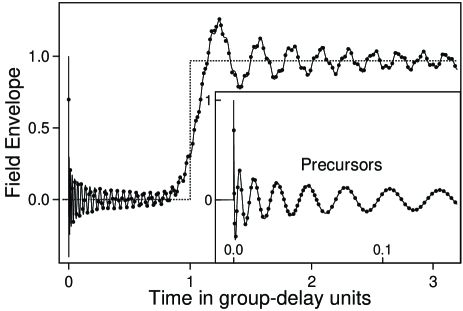
Figure 1: Step-response $a(t)$ of a medium with a natural transparency window. The analytical $\left(\bullet\right)$ and numerical (full line) forms are respectively obtained by asymptotic calculations (see text) and by the means of a FFT involving $2^{23}$ points with a time resolution of $1.2\cdot 10^{-5}\tau_{g}$. The step of amplitude $H(0)$ retarded by $\tau_{g}$ is given for reference (dotted line). Inset : enlargement of the precursors. The parameters are $\Delta=28.9\>\mathrm{ns}^{-1}$, $\gamma=0.0164\>\mathrm{ns}^{-1}$ and $\alpha L=2\cdot 10^{5}$, leading to $\tau_{g}=1.96\>\mathrm{ns}$, $H(0)=\exp(-\gamma\tau_{g})=0.968$ and $b=5.22\>\mathrm{ns}^{-1}$.

The analytical form is obtained by taking advantage of the large value of $\alpha L$. We note first that, in its very far wings, $H(\Omega)$ equals the system function of a medium with a single line of intensity optical thickness $\alpha L$ and, as expected, the short time behavior of $a(t)$ is well described by Eq.(2). For $t\geq t_{1}=\frac{1}{2\alpha L\gamma}=\frac{1}{4\Delta^{2}\tau_{g}}$, $a(t)$ can be entirely calculated by the saddle point method ble86 ; va88 . The significant contributions to $a(t)$ originates in the relevant saddle points and, eventually, in the pole at $\Omega=0$. Introducing the phase function $\Psi(\Omega)=i\Omega t+\ln\left[H\left(\Omega\right)\right]$, Eq.(1)) reads

$$a(t)=\int_{\Gamma}\exp\left[\Psi\left(\Omega\right)\right]d\Omega/2i\pi\Omega$$ (5)

The integral is calculated by deforming $\Gamma$ in a contour $\Gamma^{\prime}$ traveling along lines of steepest descent of the function $\Psi(\Omega)$ from the saddle points where $\Psi^{\prime}(\Omega)=0$ . The contribution of a non degenerate saddle point at $\Omega_{S}$ to the integral reads

$$a_{S}(t)=\left(i\Omega_{S}\sqrt{2\pi\left|\Psi^{\prime\prime}(\Omega_{S})\right|}\right)^{-1}\exp\left[\Psi\left(\Omega_{S}\right)+i\theta_{S}\right]$$ (6)

where $\theta_{S}$ is the angle of the direction of steepest descent with the real axis. Note that the instantaneous frequency of $a_{S}(t)$, defined as $d\left(\mathrm{Im}\Psi\right)/dt$ , equals $\mathrm{Re}\left(\Omega_{S}\right)$.

In the present problem, the equation $\Psi^{\prime}(\Omega)=0$ giving the saddle points can be reduced to a biquadratic equation with exact analytic solutions. The latter can be regrouped in two pairs $\Omega_{n}^{\pm}(t)=i\gamma\pm\Omega_{n}\left(t\right)$ with $n=1,2$ and

$$\Omega_{n}(t)=\Delta\sqrt{1+\left[1-\left(-1\right)^{n}\sqrt{1+8t/\tau_{g}}\right]\frac{\tau_{g}}{2t}}$$ (7)

At every time, $\Omega_{1}\left(t\right)$ is real and very large compared to $\gamma$, decreasing from $\Delta\sqrt{\tau_{g}/t}$ for $t\ll\tau_{g}$ to $\Delta$ for $t\rightarrow\infty$. The corresponding saddle points are always non-degenerate and their contribution $a_{1}\left(t\right)=a_{1}^{+}\left(t\right)+a_{1}^{-}\left(t\right)$ to $a(t)$ is easily derived from Eq.(6) with $\theta_{1}^{\pm}=\pm\pi/4$. It reads

$$a_{1}(t)\approx\sqrt{\frac{2}{\pi}}\mathrm{e}^{-\gamma t}\frac{\cos\left\{\Omega_{1}t+\Delta^{2}\tau_{g}\Omega_{1}/\left(\Omega_{1}^{2}-\Delta^{2}\right)-\pi/4\right\}}{\Omega_{1}\Delta\sqrt{\tau_{g}\left[\left(\Omega_{1}+\Delta\right)^{-3}+\left(\Omega_{1}-\Delta\right)^{-3}\right]}}$$ (8)

As expected, $a_{1}(t)$ tends to $a(t)$ given by Eq.(3) when $t\ll\tau_{g}$. More generally, $\Omega_{2}$ is purely imaginary for $t<\tau_{g}$ and the contribution of the corresponding saddle points is negligible, except in the vicinity of $\tau_{g}$. So, in a wide time-domain, $a_{1}(t)$ is actually the only significant contribution to $a(t)$. The corresponding optical field reads $E_{1}(t)=E_{1}^{+}(t)+E_{1}^{-}(t)$ where $E_{1}^{\pm}(t)=\mathrm{Re}\left[a_{1}^{\pm}(t)\exp\left(i\omega_{C}t\right)\right]$ have instantaneous frequencies $\omega_{1}^{\pm}\left(t\right)=\omega_{C}\pm\Omega_{1}\left(t\right)$. Due to the time dependence of these frequencies, $E_{1}^{+}(t)$ and $E_{1}^{-}(t)$ may be identified respectively to the Sommerfeld precursor and to the Brillouin precursor lef08 . The rise of $a\left(t\right)$ around $t=\tau_{g}$ originates from the saddle points at $\Omega_{2}^{\pm}$, which are then quasi degenerate and located in the vicinity of the pole at $\Omega=0$. The calculation of the contribution $a_{d}(t)$ to $a(t)$ of these three points requires to use an uniform asymptotic method ble86 . It is convenient to determine $a_{d}(t)$ through the corresponding contribution $h_{d}(t)$ to the impulse response $h\left(t\right)=\int_{-\infty}^{+\infty}\exp\left[\Psi\left(\Omega\right)\right]d\Omega/2\pi$. Following the procedure of ble86 ; va88 , we get $h_{d}(t)\approx b\mathrm{e}^{-\gamma t}\mathrm{Ai}\left[-b\left(t-\tau_{g}\right)\right]$ where $\mathrm{Ai}\left(x\right)$ is the Airy function and $b=\left(\Delta^{2}/3\tau_{g}\right)^{1/3}$. Finally $a_{d}(t)=\int_{-\infty}^{t}h_{d}(x)dx$ reads

$$a_{d}(t)=\mathrm{e}^{-\gamma\tau_{g}}\int_{-\infty}^{b(t-\tau_{g})}\mathrm{e}^{-\gamma x/b}\mathrm{Ai}\left(-x\right)dx\\ \approx\mathrm{e}^{-\gamma t}\int_{-\infty}^{b(t-\tau_{g})}\mathrm{Ai}\left(-x\right)dx$$ (9)

the $2^{nd}$ form holding when $\gamma\ll b$ sha08 . $a_{d}(t)$ attains its absolute maximum at the first zero of $\mathrm{Ai}\left(-x\right)$ , that is for $x\approx 2.3$ or $t=t_{2}=\tau_{g}+2.3/b$. For $t_{1}<t<t_{2}$, $a(t)$ is well fitted by $a_{1}(t)+a_{d}(t)$ (Fig.1). For $t>t_{2}$, $\Omega_{2}$ is real and the frequencies $\Omega_{2}^{\pm}$ are well separated ($\Omega_{2}\gg\gamma$). The contribution $a_{2}(t)$ of the two saddle points to $a(t)$ can then again be derived from Eq.(6) with $\theta_{2}^{\pm}=\mp\pi/4$. It reads

$$a_{2}(t)\approx-\sqrt{\frac{2}{\pi}}\mathrm{e}^{-\gamma t}\frac{\cos\left\{\Omega_{2}t+\Delta^{2}\tau_{g}\Omega_{2}/\left(\Omega_{2}^{2}-\Delta^{2}\right)+\pi/4\right\}}{\Omega_{2}\Delta\sqrt{-\tau_{g}\left[\left(\Omega_{2}+\Delta\right)^{-3}+\left(\Omega_{2}-\Delta\right)^{-3}\right]}}$$ (10)

The steepest descent contour $\Gamma^{\prime}$ passing through the four saddle points is now such that $\Gamma+\Gamma^{\prime}$ encircles the pole in $\Omega=0$. The contributions $a_{1}(t)$ and $a_{2}(t)$ should then be completed by the corresponding residue, namely $H(0)=\mathrm{e}^{-\gamma\tau_{g}}$. For $t>t_{2}$, we get thus $a(t)=\mathrm{e}^{-\gamma\tau_{g}}+a_{1}(t)+a_{2}(t)$. Again the agreement with the exact result is very good (Fig.1). The optical fields associated with $a_{2}(t)$ may be considered as second precursors but, since they arrive after the rise of the main field , we suggest to name them postcursors. Contrary to those of the precursors, their instantaneous frequencies $\omega_{2}^{\pm}\left(t\right)=\omega_{C}\pm\Omega_{2}\left(t\right)$ are initially close to $\omega_{C}$ before deviating from this frequency. Note that the oscillations in the falling tail of the pulses, observed in the experiments cama07 , are clearly related to our postcursors.

We will now examine more briefly the case of a medium with an electromagnetically induced transparency (EIT) window kasa95 ; hau99 ; boyd02 . In such a medium, precursors have been indirectly demonstrated in an experiment of two-photon coincidence du08 . We consider the simplest $\Lambda$ arrangement with a resonant control field. If the coherence relaxation rate for the forbidden transition is small enough, the medium may be transparent at $\omega_{C}$ and its system function reads

$$H\left(\Omega\right)=\exp\left\{\frac{-\alpha L\gamma/2}{i\Omega+\gamma+\Omega_{r}^{2}/4i\Omega}\right\}$$ (11)

where $\Omega_{r}$ is the modulus of the Rabi frequency of the coupling field boyd02 ; bm06 . We get then $\tau_{g}=2\alpha L\gamma/\Omega_{r}^{2}$. Fig.2 shows the step responses $a\left(t\right)$ obtained for different $\Omega_{r}$ and for a value of $\alpha L$ intermediate between those of the celebrated experiments achieved on a lead vapor kasa95 and on an ultracold gas of atomic sodium hau99 .

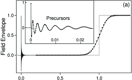
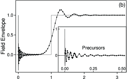
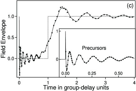
Figure 2: Same as Fig.1 for a medium with an electromagnetically induced transparency window. The parameters are $\alpha L=600$ and $\Omega_{r}/\gamma=$ (a) $4.60$ (b) $14.0$ (c) $34.6$, leading to (a) $\gamma\tau_{g}=56.7$ (b) $\gamma\tau_{g}=6.12$ and $b=1.39\gamma$ (c) $\gamma\tau_{g}=1.00$ and $b=4.64\gamma$. Note that the group delays and thus the absolute time-scales are several orders larger than in the case of the natural frequency window.

As previously and for the same reasons, the very short term behavior of $a\left(t\right)$ (up to $t_{1}=\frac{1}{2\alpha L\gamma}=\frac{1}{\Omega_{r}^{2}\tau_{g}}$) is given by Eq.(2). In general, the $4^{th}$ degree equation giving the saddle point frequencies has no simple solutions but the following properties are easily demonstrated. Irrespective of $\Omega_{r}$, $\Omega_{2}^{-}(\tau_{g})=0$ and, for $t\rightarrow 0$, $\Omega_{1}^{\pm}\left(t\right)\rightarrow i\gamma\pm\Omega_{r}\sqrt{\tau_{g}/4t}$ while $\Omega_{2}^{\pm}\left(t\right)\rightarrow\pm i\Omega_{r}/2$. When $\Omega_{r}<\gamma$, $\Omega_{2}^{+}\left(t\right)$ and $\Omega_{2}^{-}\left(t\right)$ keep non degenerate and purely imaginary at every time. If on the contrary $\Omega_{r}>\gamma$, these two frequencies coalesce at a time $t_{d}>\tau_{g}$ in $\Omega_{d}=i\Omega_{r}\sin\left[\sin^{-1}\left(\gamma/\Omega_{r}\right)/3\right]$. For $\Omega_{r}>4\gamma$, $\Omega_{d}\approx i\gamma/3$ and $t_{d}=\tau_{g}\left(1+4\gamma^{2}/3\Omega_{r}^{2}\right)$. Explicit analytical expressions of $a(t)$ can be obtained when $\Omega_{r}/\gamma$ is moderate or large.

In the first case, $\gamma\tau_{g}=2\alpha L\gamma^{2}/\Omega_{r}^{2}\gg 1$ and the precursors will have a short duration compared to $\tau_{g}$. In this time domain $\Omega_{1}^{\pm}\left(t\right)\approx i\gamma t\pm\Omega_{r}\left(1+3t/2\tau_{g}\right)\sqrt{\tau_{g}/4t}$ and

$$a_{1}(t)\approx\sqrt{\frac{2}{\pi}}\mathrm{e}^{-\gamma t}\frac{\cos\left[\Omega_{r}\left(1+t/2\tau_{g}\right)\sqrt{t\tau_{g}}-\pi/4\right]}{\left(\Omega_{r}\sqrt{t\tau_{g}}\right)^{1/2}}$$ (12)

If $\gamma\tau_{g}$ is extremely large, the term $t/2\tau_{g}$ may be neglected and $a_{1}(t)$ again equals $a(t)$ given Eq.(3). This particular case is examined in du09 . When $\Omega_{r}\leq\gamma$ or when $\Omega_{r}>\gamma$ with $\gamma\left(t_{d}-\tau_{g}\right)\gg 1$ (Fig.2a), the only other significant contribution to $a\left(t\right)$ is $a_{2}^{-}\left(t\right)$ associated with the saddle point at $\Omega_{2}^{-}\left(t\right)$ which tends to $0$ for $t\rightarrow\tau_{g}$. We circumvent the difficulty due to the coincidence of the saddle point with a pole by passing through the associated impulse response $h_{2}^{-}\left(t\right)$. It reads $h_{2}^{-}\left(t\right)=\left(\sqrt{2\pi\left|\Psi"\left(\Omega_{2}^{-}\right)\right|}\right)^{-1}\exp\left[\Psi\left(\Omega_{2}^{-}\right)+i\theta_{2}^{-}\right]$ with $\theta_{2}^{-}=0$, $\Psi\left(\Omega_{2}^{-}\right)\approx-\left[\Omega_{r}\left(t-\tau_{g}\right)/4\sqrt{\gamma\tau_{g}}\right]^{2}$ and $\Psi"\left(\Omega_{2}^{-}\right)\approx-8\gamma\tau_{g}/\Omega_{r}^{2}$. We finally get

$$a_{2}^{-}\left(t\right)=\frac{1}{2}\left(1+\mathrm{erf}\left[\Omega_{r}\left(t-\tau_{g}\right)/4\sqrt{\gamma\tau_{g}}\right]\right)$$ (13)

where $\mathrm{erf}(x)$ is the error function. $a_{2}^{-}\left(t\right)\rightarrow 1$ when $\Omega_{r}\left(t-\tau_{g}\right)\gg 4\sqrt{\gamma\tau_{g}}$ and $a_{1}\left(t\right)+a_{2}^{-}\left(t\right)$ provides a good approximation of the exact step response at every time (Fig.2a).

When $\Omega_{r}\gg\gamma$ the coupling field splits the original line in a doublet of lines approximately centered at $\omega_{C}\pm\Omega_{r}/2$. If, in addition, $\left(\Omega_{r}/\gamma\right)^{4}\gg 8\alpha L/3$ , then $\gamma\left(t_{d}-\tau_{g}\right)\ll 1$ and the situation is analogous (but not identical) to that encountered with a natural transparency window. The frequencies of the saddle points approximately equal $\Omega_{n}^{\pm}\approx i\gamma_{n}\left(t\right)\pm\Omega_{n}\left(t\right)$ where $\gamma_{n}\left(t\right)\approx\left(\gamma/2\right)\left[1-\left(-1\right)^{n}\left(1+8t/\tau_{g}\right)^{-1/2}\right]$ and where $\Omega_{n}\left(t\right)$ is given by Eq.(7), with $\Delta=\Omega_{r}/2$. The different contributions to $a\left(t\right)$ then read

$$a_{1}(t)\approx\sqrt{\frac{2}{\left|\pi\Psi"\left(\Omega_{1}^{+}\right)\right|}}\mathrm{Re}\left\{\frac{1}{\Omega_{1}^{+}}\mathrm{e}^{\left[\Psi\left(\Omega_{1}^{+}\right)-i\pi/4\right]}\right\}$$ (14)

$$a_{2}(t)\approx-\sqrt{\frac{2}{\left|\pi\Psi"\left(\Omega_{2}^{+}\right)\right|}}\mathrm{Re}\left\{\frac{1}{\Omega_{2}^{+}}\mathrm{e}^{\left[\Psi\left(\Omega_{2}^{+}\right)+i\pi/4\right]}\right\}$$ (15)

$$a_{d}\left(t\right)\approx\int_{-\infty}^{b\left(t-\tau_{g}\right)}\mathrm{Ai}\left(-x\right)\exp\left(-\gamma x/3b\right)dx$$ (16)

where $b=\left(\Omega_{r}^{2}/12\tau_{g}\right)^{1/3}$. As in the case of the natural frequency window, $a_{1}\left(t\right)+a_{d}\left(t\right)$ and $a_{1}\left(t\right)+a_{2}\left(t\right)+H(0)$ fit very well the exact step response, respectively for $t_{1}<t<t_{2}=\tau_{g}+2.3/b$ and for $t>t_{2}$ (Fig.2b and Fig.2c). The main difference is that a significant damping of the precursors is now compatible with a good transparency at $\omega_{C}$. For intermediate values of $\Omega_{r}$ it is so possible to observe both well developed precursors and postcursors without overlapping (Fig.2b). On the contrary, the tail of the precursors again partially interferes with the postcursors for very large $\Omega_{r}$(Fig.2c).

To conclude, we have obtained, for the first time, fully analytic expressions of the entirety of the step response of linear media with a transparency window. Our results show that these media, contrary to those generally considered, are well adapted to observe in a same experiment the precursors, the main field and the postcursors, all well distinguishable from each other and having comparable amplitudes. Insofar as the parameters used in the calculations are representative of real experiments, we think that our work might stimulate an experimental observation of these rich dynamics, which would, in turn, stimulate new theoretical investigations on related slow-light systems.

References

(1) A. Sommerfeld, Ann. Phys. (Leipzig) 44, 177 (1914).
(2) L. Brillouin, Ann. Phys. (Leipzig) 44, 204 (1914).
(3) An English translation of som14 and bri14 can be found in : L. Brillouin, Wave Propagation and Group Velocity(Academic Press, New York, 1960).
(4) J.A. Stratton, Electromagnetic Theory (McGraw-Hill, New York 1941)
(5) J.D. Jackson, Classical Electrodynamics, 2nd ed. (Wiley, New York 1975).
(6) K.E. Oughstun and G.C. Sherman, Pulse Propagation in Causal Dielectrics (Springer, Berlin 1994).
(7) K.E. Oughstun, Electromagnetic and Optical Pulse Propagation 1 (Springer, Berlin 2007), Ch.1.
(8) K.E. Oughstun, J. Opt. Soc. Am. A, 12, 1715 (1995).
(9) P. Pleshko and I. Palócz, Phys. Rev. Lett. 22, 1201 (1969).
(10) J. Aaviksoo, J. Kuhl, and K. Ploog, Phys. Rev. A 44, R5353 (1991).
(11) M.Sakai et al., Phys.Rev.B 66, 033302 (2002).
(12) U. Österberg, D. Andersson, and M. Lisak, Optics Com. 277, 5 (2007)
(13) We use the definitions and sign conventions of A.Papoulis, The Fourier Integral and its applications (Mc Graw Hill, New York 1987)
(14) E. Varoquaux, G. A. Williams, and O. Avenel, Phys. Rev. B 34, 7617 (1986). See Eq.(49).
(15) B. Ségard, J. Zemmouri, and B. Macke, Europhys. Lett. 4, 47 (1987). See Fig.2.
(16) H. Jeong, A. M. C. Dawes, and D.J. Gauthier, Phys. Rev. Lett., 96, 143901 (2006).
(17) W.R. LeFew, S. Venakides, and D.J. Gauthier, e-print ArXiv 0705.4238v3.
(18) H. Tanaka et al., Phys. Rev. A 68, 053801 (2003).
(19) R.M. Camacho, M.V. Pack, and J.C. Howell, Phys. Rev. A 73, 063812 (2006).
(20) R.M. Camacho et al., Phys. Rev. Lett. 98, 153601 (2007).
(21) M.R. Vanner, R.J. McLean, P. Hannaford, and A.M. Akulshin, J. Phys. B : At. Mol. Opt. Phys. 41, 051004 (2008).
(22) B. Macke and B. Ségard, Phys. Rev. A 73, 043802 (2006).
(23) The results derived from Eq.(3) hold even if the two lines are not Lorentzian provided that they are so in their wings cama07 . The optical thickness intervening in this equation may then be considerably larger than its actual value on resonance.
(24) N. Bleistein and R.A. Handelsman, Asymptotic Expansions of Integrals (Dover, New York 1986).