A Wide-field High Resolution H I Mosaic of Messier 31
I. Opaque Atomic Gas and Star Formation Rate Density

Abstract

We have undertaken a deep, wide-field H I imaging survey of M31, reaching a maximum resolution of about 50 pc and 2 km s^-1 across a 95$\times$48 kpc region. The H I mass and brightness sensitivity at 100 pc resolution for a 25 km s^-1 wide spectral feature is 1500 M_⊙ and 0.28 K. Our study reveals ubiquitous H I self-opacity features, discernible in the first instance as filamentary local minima in images of the peak H I brightness temperature. Local minima are organized into complexes of more than kpc length and are particularly associated with the leading edge of spiral arm features. Just as in the Galaxy, there is only patchy correspondence of self-opaque features with CO(1-0) emission. We have produced images of the best-fit physical parameters; spin temperature, opacity-corrected column density and non-thermal velocity dispersion, for the brightest spectral feature along each line-of-sight in the M31 disk. Spectroscopically opaque atomic gas is organized into filamentary complexes and isolated clouds down to 100 pc. Localized opacity corrections to the column density exceed an order of magnitude in many cases and add globally to a 30% increase in the atomic gas mass over that inferred from the integrated brightness under the usual assumption of negligible self-opacity. Opaque atomic gas first increases from 20 to 60 K in spin temperature with radius to 12 kpc but then declines again to 20 K beyond 25 kpc. We have extended the resolved star formation law down to physical scales more than an order of magnitude smaller in area and mass than has been possible previously. The relation between total-gas-mass- and star-formation-rate-density is significantly tighter than that with molecular-mass and is fully consistent in both slope and normalization  with the power law index of 1.56 found in the molecule-dominated disk of M51 at 500 pc resolution. Below a gas-mass-density of about 5 M_⊙pc^-2, there is a down-turn in star-formation-rate-density which may represent a real local threshold for massive star formation at a cloud mass of about 5$\cdot 10^{4}$ M_⊙.

1 Introduction

As the nearest major external galaxy and possibly the dominant member of the Local Group, Messier 31 has received a great deal of attention since its’ first documented telescopic observation by Simon Marius in 1612 (Marius, 1612). The many stellar and gaseous constituents of M31 continue to be studied with ever greater sensitivity and resolution, permitting insights that are in many cases difficult or even impossible to achieve for our own Galaxy given our vantage point within the disk. One of these areas, where an external yet nearby vantage point is crucial to achieving a global overview, is the study of the neutral interstellar medium. Although we can achieve remarkable physical sensitivity and resolution of the neutral medium of the Galaxy, resolving individual structures of 100’s of AU in size and as little as several Jupiter masses (Braun & Kanekar, 2005), it is very difficult to estimate even the total mass of the neutral medium, let alone its overall distribution and relationship with other components. Studies of the neutral medium of M31 began with the pioneering work of Van de Hulst et al. (1957) as one of the first programs undertaken with the Dwingeloo 25m telescope. Subsequent studies with larger single dishes and then with interferometric arrays have provided enhanced resolution and brightness sensitivity, although the highest resolution studies have often only been directed at a portion of the disk (eg. Brinks & Shane (1984), Braun (1991), Carignan et al. (2006)).

In this paper we describe our Westerbork and Green Bank Telescope program to image the entire atomic disk of M31 with a uniformly high sensitivity and resolution. The most recent effort on a comparable scale was that of Unwin (1983) which achieved arcmin spatial and 16 km s^-1 velocity resolution with an RMS noise of 3.6 K in two elliptical fields covering about 12 square degrees. By contrast we will present imaging down to 15” spatial and 2.3 km s^-1 velocity resolution (sampled at 2 km s^-1) with a uniform 2.7 K RMS over a region of about 24 (7$\times$3.5) square degrees. This corresponds to a maximum linear resolution of about 50 pc over a total extent of more than 90 kpc. With even modest spatial smoothing we reach sub-Kelvin brightness sensitivity (for example 0.37 K at 1 arcmin), making our database the most detailed documentation yet of the neutral medium of any complete galaxy disk, including our own. For comparison, the Leiden/Argentine/Bonn Survey of Galactic H I has achieved 36 arcmin and 1.3 km s^-1 resolution over 360 degrees and reaches 0.08 K RMS Kalberla et al. (2005) and the Large Magellanic Cloud survey of Kim et al. (2003) achieves 1 arcmin and 1.7 km s^-1 resolution over 12$\times$10 degrees and reaches 2.5 K RMS.

We begin with a description of the observations and their reduction in §2 and continue with an overview of the results in §3. In §4 we present some initial analysis of the data, beginning with a discussion of H I self-opaque features and followed by a detailed fitting of all high signal-to-noise spectra to determine the best fitting combination of the physical parameters along each line-of-sight: cool component temperature, total column density and non-thermal velocity dispersion. We continue with the analysis of radial dependence for the relevant physical parameters and finally we focus on the relationship between surface density of gas mass and star formation rate. We close with some brief conclusions in §5. We assume a distance to M31 of 785 kpc (McConnachie et al., 2005) throughout.

Further papers in this series will include: (1) a detailed kinematic- and mass-model of M31, (2) comparative studies of the morphology of the inner and outer disks and (3) a study of small-scale kinematic features such as outflows and other peculiar velocity components.

2 Observations and Reduction

Interferometric observations of the extended M31 H I disk with the Westerbork Synthesis Radio Telescope (WSRT) array were obtained on a Nyquist sampled (15 arcmin spacing) pointing grid defined in the M31 (major, minor) axis coordinate system. The disk extent was first determined in a precursor total power survey which fully sampled a 6$\times$6 degree field at low resolution (36’ FWHM) using the 14 individual telescopes of the WSRT array. A total of 163 synthesis pointing positions were chosen from the grid to provide good coverage of the region of anticipated H I emission. Observations were then obtained for 27 tracks of 12 hour duration with the WSRT array, each sampling 6 (or in one case 7) different pointing positions. These data were observed between August 2001 and January 2002. Each 12 hour track involved cycling through the 6 relevant pointing positions with a series of 10 minute snap-shots. The tracks were preceeded by half hour observations of the calibration sources 3C286 and CTD93 and followed by half hour observations of 3C147 and CTA21. A total band-width of 5 MHz (covering heliocentric radial velocities between $-$828 and $+$227 km s^-1) was observed with 512 spectral channels in two linear polarization products yielding a channel width of 2.06 km s^-1 and resolution of 2.27 km s^-1. Calibration and flagging of the data were done in Classic AIPS. After external band-pass and gain calibration, each pointing was self-calibrated using the continuum emission which happened to be present. The continuum model was subtracted from the visibilities and residual continuum was removed with UVLIN.

Sensitive total power data covering a 7$\times$7 degree field was acquired with the Green Bank Telescope (GBT) telescope over six nights in September 2002. These data, with 9$\farcm$1 FWHM $\times$ 1.03 km s^-1 resolution and an RMS sensitivity in H I column density over relevant linewidths of about 5$\times 10^{17}$ cm^-2, have already been presented in Thilker et al. (2004).

A joint deconvolution of all 163 pointings was done with the Miriad (Sault et al., 1995) task MOSSDI, after forming a weighted sum of the linearly combined synthesis image (employing uniform weighting followed by a Gaussian taper) with the relevant GBT total power image. Each of the 163 synthesized beams was also modified by addition of a Gaussian approximation of the total power beam using the same relative weightings as used when summing the synthesis and total power images. The relative weightings were determined empirically by minimizing the “short-spacing bowl” effect in the synthesis beams, but they correspond roughly to the inverse of the relative beam areas. The exact choice of weighting is not critical, in theory, since the process of deconvolution should yield an “ideal” final PSF if all emission has been successfully incorporated into the component model. In practise it is never possible to incorporate all emission into the component model, so it is important to make the “dirty” PSF as clean as possible (particularly with respect to diffuse emission) by an optimized choice of weights.

The linearly combined “dirty” mosaic images were multiplied with the combined WSRT survey sensitivity pattern in order to weight down the noise around the periphery of the sampled region before deconvolution. If this were not done, then the noisy periphery would be severely over-CLEANed relative to the central regions, yielding greatly reduced image fidelity. The assumption underlying this spatial tapering is that the region of significant emission is contained within the sampling pattern. We will comment below on the extent to which this assumption was met in practise. The 300 semi-independent spectral channels (each of 2 km s^-1 width) containing M31’s H I emission (heliocentric velocities of about $-$621 to $-$20 km s^-1) were processed individually. Foreground H I emission from the Galaxy is present in the field of M31 at velocities between about $-$130 and $+$45 km s^-1. Reduction of the WSRT data over the full velocity range of Galactic emission was not undertaken at this time. The GBT total power images at velocities between $-$130 and $-$20 km s^-1 were modified by subtraction of the median value determined outside of the region occupied by the M31 disk before combination with the WSRT mosaic to simplify the deconvolution problem. A positive pedestal of emission underlying the entire galaxy is a needless complication that undermines image fidelity in the deconvolved result.

Given the non-linear nature of the deconvolution process and the desire to probe a variety of different output spatial (“full”=18$\farcs$4$\times$14$\farcs$8 (NS$\times$EW), 30″, 60″and 120″) and velocity (2.3, 6.2, 10.3, and 18.5 km s^-1) resolutions, we carried out the joint deconvolution independently for each different combination of these parameters. Deconvolution was in all cases done to a depth of twice the theoretical RMS noise level at each resolution. A bug in the MOSSDI source code was remedied (affording it protection against a negative loop gain). A small adjustment was also made to the primary beam model employed within Miriad for the WSRT telescopes. It was found empirically, that a small increase (by 5 %) in the assumed FWHM of the analytic approximation ($cos^{6}(C\cdot\nu\cdot r)$ for a constant $C$ at frequency $\nu$ in terms of the radius $r$) for the beam pattern yielded the highest dynamic range in the mosaic result. The slightly larger than expected beam size (2110 arcsec FWHM rather than 2013 arcsec at 1420 MHz) has since been verified by direct measurement (Popping & Braun, 2008). The resulting RMS noise levels at various spatial and velocity resolutions are listed in Table 1. Note that unlike the case of total power observations of Galactic H I, the detected M31 H I emission in our synthesis images does not contribute significantly to the measured antenna temperature of each dish, and therefore does not give rise to an increase of the system temperature.

Table 1: RMS Sensitivity at Various Resolutions

Resolution			RMS Sensitivity
Beam	$\Delta V$		$\Delta S$	$\Delta T_{B}$	$\Delta N_{HI}$	$\Delta M_{HI}$
[arcsec]	[km s-1]		[mJy/Beam]	[K]	[1018cm-2]	[M⊙]
18$\times$15	2.3		1.2	2.7	11.3	390
30	2.3		1.5	1.0	4.2	490
60	2.3		2.2	0.37	1.6	720
120	2.3		4.2	0.15	0.63	1400
18$\times$15	18.5		0.42	0.95	32	1100
30	18.5		0.53	0.35	11.8	1400
60	18.5		0.78	0.13	4.4	2100
120	18.5		1.5	0.053	1.8	4000

A locally modified version of Miriad was employed that contains many enhancements for high performance computing. It extensively exploits parallelism at several levels: multi-threading (on machines that have multiple CPUs) and vectorization (using SSE (Streaming SIMD Extensions) instructions which are available on most contemporary processors). Furthermore, we used task-level parallelism by dividing different reduction pipelines (specific resolutions and spectral channels) over multiple machines. The “Netherlands Grid” infrastructure provided us with the resources to do the computational work. Using these techniques, we were able to perform all reductions (16 different resolutions, 300 semi-independent spectral channels) in 36 hours of elapsed time. A previous attempt to carry out the same processing, before code optimization and using only a single high-end server, required several months of elapsed time.

Although data products at all 16 different resolutions were generated directly from the visibility data, we also produced velocity-averaged data products at a fixed spatial resolution by averaging the individually processed channels after deconvolution. Superior dynamic range was found for these post-deconvolution averaged products at spatial resolution of both 60 and 120 arcseconds, while the directly imaged products were superior at full and 30 arcsecond resolutions. Apparently, different deconvolution limitations dominate in these two regimes. At high spatial resolutions, the increased signal-to-noise ratio afforded by visibility-based velocity smoothing improves the recovery of extended emission structures, while at low spatial resolutions we already encounter the finite image fidelity of the deconvolution in an individual velocity channel. In this case, averaging spectral images after deconvolution can improve the dynamic range of the result. The nominal RMS noise levels after spectral smoothing scale simply with the square root of the eventual velocity resolution. H I column density sensitivity at an appropriate spectral smoothing for faint emission features (of 18.5 km s^-1) is tabulated in Table 1 at a series of spatial resolutions.

Images of the peak observed line brightness and the integrated brightness and associated mean velocity (the 0^th and 1^st moments) were produced at each resolution after first masking the data-cube. The mask was constructed from the cube of 120 arcsec and 18 km s^-1 resolution, by first blanking brightnesses below 1.5$\sigma$ and then interactively masking with an arbitrary polygon the “island” of most significant emission at each velocity. Interactive isolation of M31 H I emission was most critical in the velocity range that overlaps that of the Galaxy ($-$130 to $-$20 km s^-1). Subtraction of the off-M31 median total power before deconvolution already served to place the M31 emission on a plausible base level. Only a single contiguous (both spatially and in velocity) “island” of emission at each velocity was included in the blanking mask. Although isolated features in the field may be associated with M31, we are unaware of how to distinguish them from features in the Galactic foreground. All features in the field which were not contiguously connected with the M31 disk emission were presumed to be part of the Galactic foreground and were excluded.

Images of integrated brightness were rescaled to represent column density assuming a negligible H I line opacity. Although this is the usual assumption, it is clear that it is incorrect in practise. Braun & Walterbos (1992) have applied a simple, single temperature opacity correction to the observed H I brightnesses from the North-East half of M31 and find local corrections of a factor of 2 and an integrated correction of some 20%. We address the issue of H I opacity in greater detail below by directly fitting physical models to individual spectra for all lines-of-sight.

Another useful type of image for diagnostic purposes is that of “velocity coherence” (VC) (as first introduced by Braun (1997)), defined as the ratio of peak brightness at two different spectral resolutions. For example, VC${}_{30/5}(x,y)~{}=~{}P_{30}(x,y)$ / $P(_{5}x,y)$, where $P_{R}(x,y)$ is the peak brightness observed at a spectral resolution of $R$ km s^-1. In the absence of noise, $0\leq VC\leq 1$, when comparing coarser with finer spectral resolutions, since an infinitely broad spectral feature will always retain the same peak brightness (VC = 1), while an extremely narrow feature will be strongly diluted (VC $\rightarrow$ 0). Images of velocity coherence are a robust measure of linewidth, since no assumption regarding the intrinsic line-shape, nor reliance on a fitting algorithm are required for it’s calculation. Moreover, even when spectra become multi-valued, as they do in highly inclined (like M31) or kinematically disturbed systems, the VC can continue to probe the attributes of the dominant spectral feature along each line-of-sight rather than a smeared version of all spectral content. In the particular case of an intrinsically Gaussian line profile with dispersion, $\sigma$, that is fully resolved at the higher resolution and then convolved with a Heaviside (top-hat) function of width, $\Delta V$, one gets the relation, $\sigma=\Delta V\cdot VC/[(1-VC)\sqrt{2\pi}]$.

3 Overview of Results

An overview of the joint deconvolution result is shown in Figure 1 where the WSRT mosaic sensitivity pattern is overlaid on a low resolution (120 arcsec, 10 km s^-1) image of peak H I brightness. The Karma package (Gooch, 1996) has been employed for many of the illustrations. Sensitivity contours are shown at 10 and 50% of the peak sensitivity which results from the sampling pattern. The combined sensitivity pattern has what turn out to be unfortunate local minima on either side of the minor axis. Although little evidence for emission was discerned at these locations in our pilot WSRT total power observations, it is clearly present in the more sensitive total power data that we have acquired since (Thilker et al. (2004) and Braun & Thilker (2004)). Diffuse patches of emission are apparent on both sides of the minor axis. The apparent termination of these minor axis extensions is likely influenced by the multiplication of the brightness distribution with the sensitivity pattern (to control noise amplification during deconvolution, as outlined in §2 above). More extensive sampling of the minor axis with additional mosaic pointings will be required for high fidelity imaging at arcmin resolution. Our total power data (with up to 9 arcmin resolution) do not suffer from this limitation. Similar attenuation affects Davies’ Cloud (Davies (1975), De Heij et al. (2002)) the diffuse structure at $\delta$=42$\fdg$5 to the northwest of the M31 disk. The southernmost of the H I clumps at $\delta$=38$\fdg$8 and due South of M31 (Thilker et al., 2004) is also somewhat attenuated. Sensitive pointed observations of these features are presented in Westmeier et al. (2005).

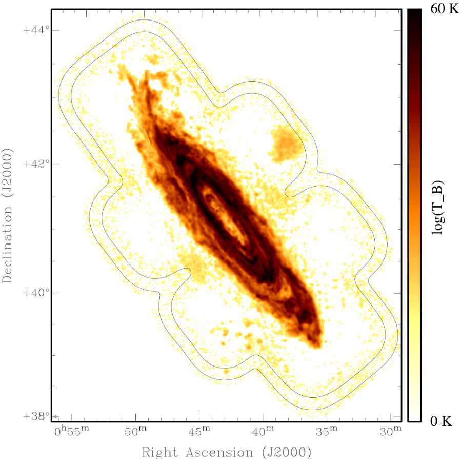
Figure 1: Peak brightness of H I emission determined at 120 arcsec and 10 km s^-1 resolution is overlaid with the combined sensitivity pattern of the 163 pointings in the mosaic observation. Contours are drawn at 10 and 50% of the peak sensitivity. Peak brightness is shown on a logarithmic scale which saturates at 60 K. The beam FWHM is indicated in the lower left corner.

Greater detail can be discerned in Figure 2 in which peak brightness is shown as determined at 60 arcsec (220 pc) and 6 km s^-1 resolution, although even at this modest resolution, the PSF (plotted in the lower left corner of the image) is barely resolved on a printed page, given that the image spans 111 kpc across the diagonal. Zooming in at this resolution on the central disk as in Figure 3 finally permits appreciation of which features are resolved. Jumping now to 30” (110 pc) resolution on the same field in Figure 4 begins to reveal the intricate filamentary structure of the neutral ISM. Point-like local minima are seen toward the most prominent background sources (J004218+412926 and J004648+420855) against which H I absorption is detected. Increasing the angular resolution to the maximum available of about 55 pc (18.4$\times$14.8 arcsec) as in Figure 5 does not appear to appreciably add detail to the filamentary structure, while increasing the noise level significantly. This is consistent with what was found by Braun (1995) when analyzing H I emission data from the northeast half of the inner M31 disk; beginning with data having 10” and 5 km s^-1 resolution, spatial smoothing to 40” resolution was required before the mean peak detected brightness decreased by 8%, while velocity smoothing to even 10 km s^-1 resulted in a mean decrease of peak brightness of 15%. The major H I cloud complexes which are discernable in external galaxies with current instrumentation are essentially resolved with about 100 pc and 5 km s^-1 resolution. However, it must also be stressed that significant structure is present at even the highest angular and velocity resolution that is available. We will briefly discuss some examples in §4 below.

Continuing on from the best signal-to-noise inner disk overview of Figure 4, further magnification is required to discern individual features on a printed page. The three images in Figs. 6–8 give some appreciation of the wealth of detail which can be discerned in the inner disk of M31. Peak H I brightness is shown in the left hand panels of each figure, while velocity coherence VC_18.5/2.1 (defined in §2) for the same region is shown on the right. A striking aspect of these images is the appearance of filament-like minima as well as positive morphological features, as seen in peak brightness. While positive emission features are not surprising when imaging the H I distribution of an external galaxy, the filamentary minima are quite novel. A further striking feature is the correspondence of high velocity coherence with the majority of these local minima. Apparently the filamentary features having depressed peak brightness are often accompanied by a substantial broadening of the underlying spectral profile. This trend is illustrated in Figs. 9 and 10 (at 30″and 2.3km s^-1 resolution), where sequences of spectra are shown which contrast the appearance of these local minima (central panels) with flanking spectra which are offset perpendicular to each “dark” filament by only about 30 arcsec (left and right panels). The locations of these cross-cuts are shown in Figs. 6, 7 and 8. From these spectra it is apparent that the line profiles toward such local minima in peak brightness are not only broad, but have a distinctive flat-topped appearance that is strongly suggestive of self-opacity in the emission line. The smooth curves overlaid on each spectrum are the parameterized model-fits to each spectrum that we describe in detail below in §4.2. Note that the RMS sensitivity of these spectra, is that given in Table 1 of about 1 K, implying that some of the fluctuations seen toward the flat-topped peaks are quite significant. The parameterized fits are indeed consistent with a significant self-opacity of the H I emission within this entire system of filamentary local minima.

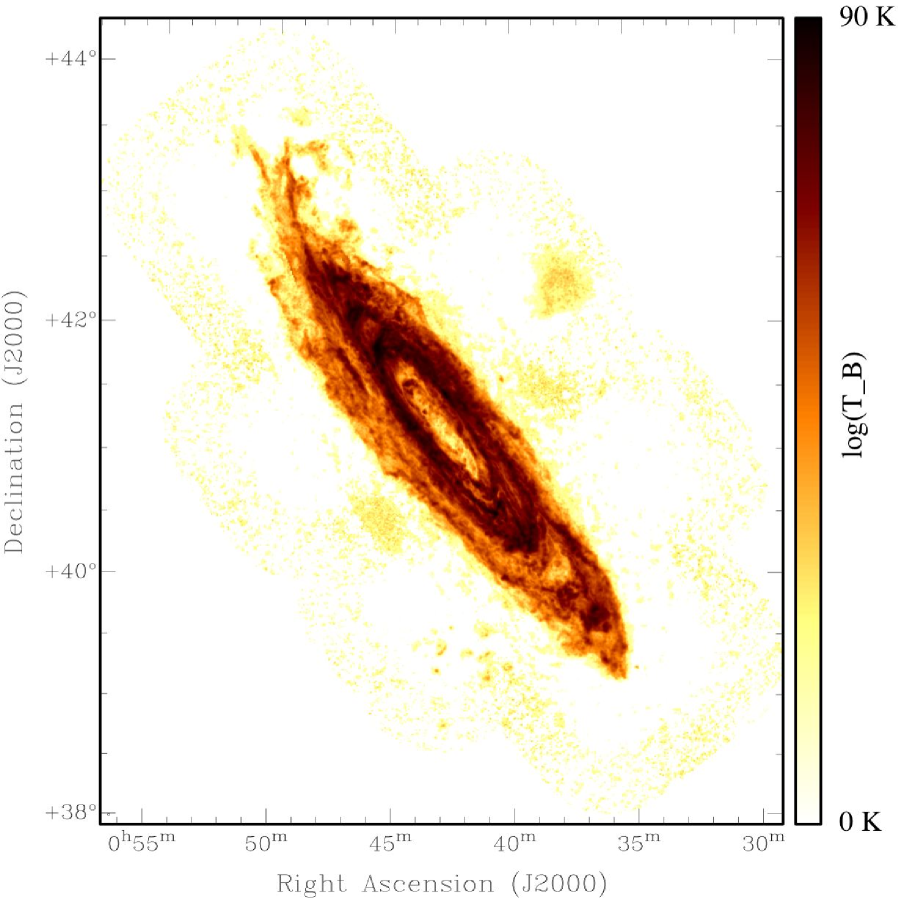
Figure 2: Peak brightness of H I emission determined at 60 arcsec and 6 km s^-1 resolution. Peak brightness is shown on a logarithmic scale which saturates at 90 K. The beam FWHM is indicated in the lower left corner.

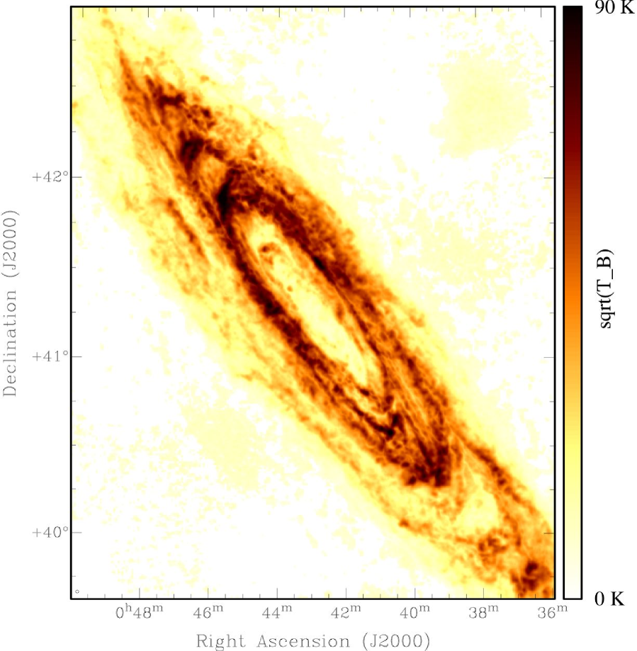
Figure 3: Peak brightness of H I emission determined at 60 arcsec and 6 km s^-1 resolution of the central 50% of the survey region. Peak brightness is shown on a square-root scale which saturates at 90 K. The beam FWHM is indicated in the lower left corner.

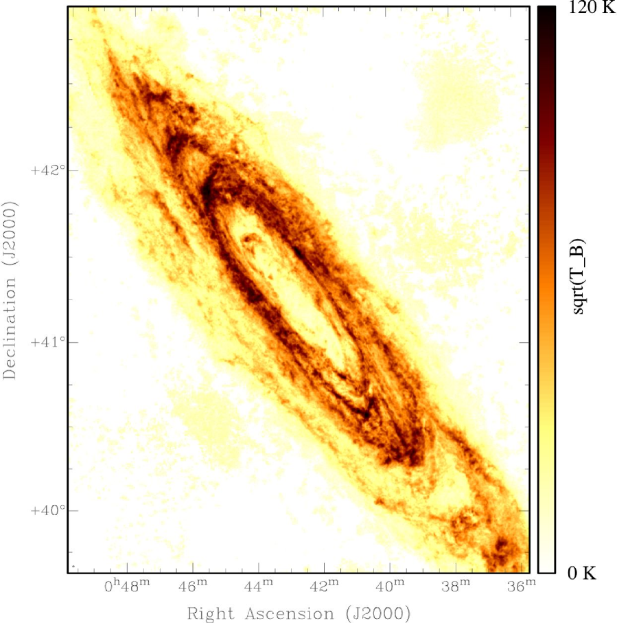
Figure 4: Peak brightness of H I emission determined at 30 arcsec and 6 km s^-1 resolution of the central 50% of the survey region. Peak brightness is shown on a square-root scale which saturates at 120 K. The beam FWHM is indicated in the lower left corner.

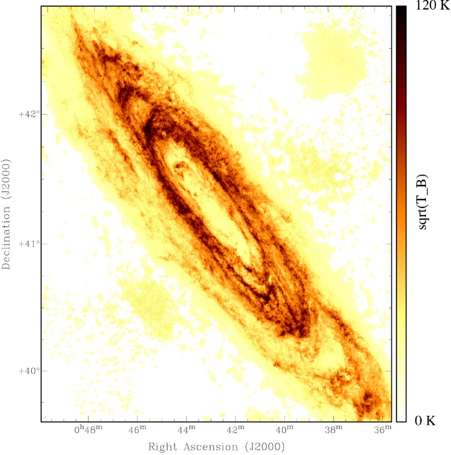
Figure 5: Peak brightness of H I emission determined at about 15 arcsec and 6 km s^-1 resolution of the central 50% of the survey region. Peak brightness is shown on a square-root scale which saturates at 120 K. The beam FWHM is indicated in the lower left corner.

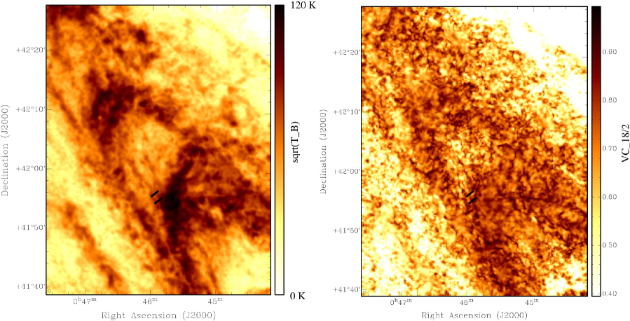
Figure 6: Peak brightness (left) and velocity coherence (right) of H I emission determined at 30 arcsec resolution of the North-East disk region. Peak brightness is shown on a square-root scale which saturates at 120 K. Velocity coherence (defined in the text) is measured between 18.5 and 2.1 km s^-1 spectral smoothing. The black bars indicate the location of the spectra shown in Fig. 9. The beam FWHM is indicated in the lower left corner.

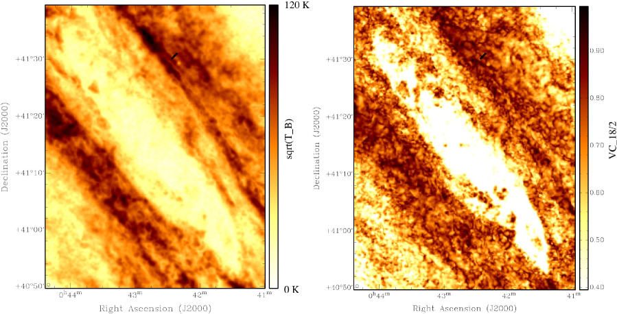
Figure 7: Peak brightness (left) and velocity coherence (right) of H I emission determined at 30 arcsec resolution of the central survey region. Peak brightness is shown on a square-root scale which saturates at 120 K. Velocity coherence (defined in the text) is measured between 18.5 and 2.1 km s^-1 spectral smoothing. The black bar indicates the location of the spectra shown in Fig. 9. The beam FWHM is indicated in the lower left corner.

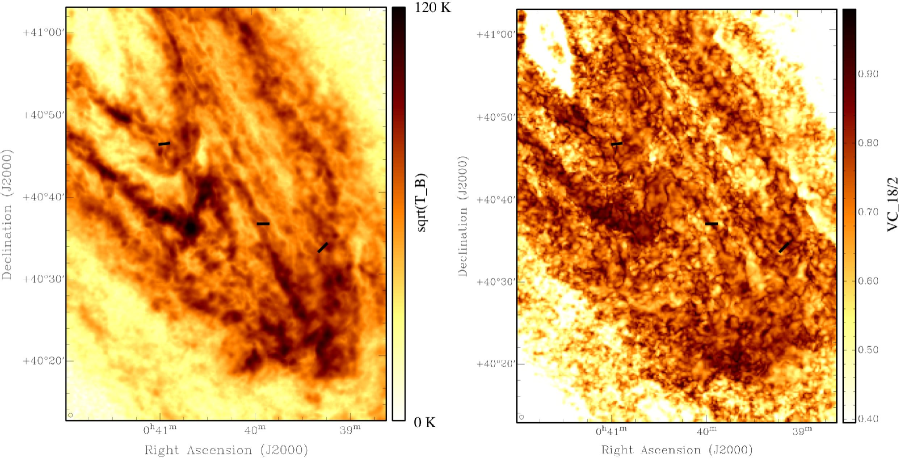
Figure 8: Peak brightness (left) and velocity coherence (right) of H I emission determined at 30 arcsec resolution of the South-West disk region. Peak brightness is shown on a square-root scale which saturates at 120 K. Velocity coherence (defined in the text) is measured between 18.5 and 2.1 km s^-1 spectral smoothing. The black bars indicate the location of the spectra shown in Fig. 10. The beam FWHM is indicated in the lower left corner.

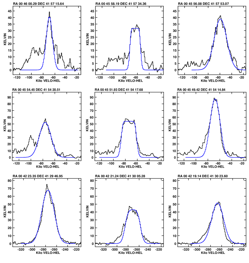
Figure 9: H I spectra of dark filaments. The three sequences of spectra (top, middle and bottom) each represent a cross-cut perpendicular to a filamentary local minimum in the image of peak brightness temperature shown in Figs. 6 and 7. The spectrum in each central panel is in the direction of the dark filament, while the left and right spectra are offset by about 30 arcsec (as indicated by the coordinates). The resolution is 30″and 2.3 km s^-1. Note the depressed, flat-topped profiles toward the filament, flanked by brighter, more smoothly peaked profiles. The smooth curve overlaid on each spectrum is the parameterized fit.

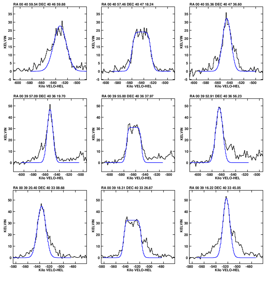
Figure 10: H I spectra of dark filaments. The three sequences of spectra (top, middle and bottom) each represent a cross-cut perpendicular to a filamentary local minimum in the image of peak brightness temperature shown in Fig. 8. The spectrum in each central panel is in the direction of the dark filament, while the left and right spectra are offset by about 30 arcsec (as indicated by the coordinates). The resolution is 30″and 2.3 km s^-1. Note the depressed, flat-topped profiles toward the filament, flanked by brighter, more smoothly peaked profiles. The smooth curve overlaid on each spectrum is the parameterized fit.

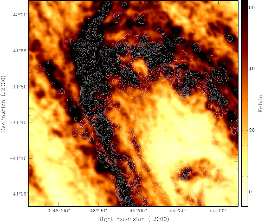
Figure 11: Peak brightness of H I emission determined at 30 arcsec and 6 km s^-1 resolution of the North-East disk region with contours of integrated CO(1-0) (from (Nieten et al., 2006)) superposed at $2.34\times 1.2^{n}$ K-km/s, for n=1,2,3$\dots$.

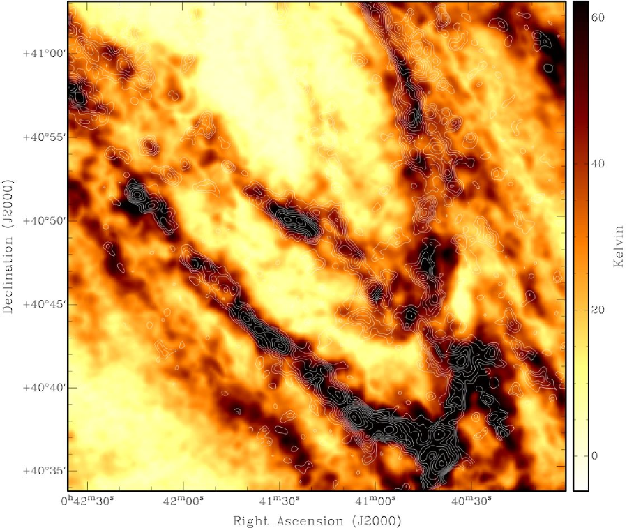
Figure 12: Peak brightness of H I emission determined at 30 arcsec and 6 km s^-1 resolution of the South-West disk region with contours of integrated CO(1-0) (from (Nieten et al., 2006)) superposed at $2.34\times 1.2^{n}$ K-km/s, for n=1,2,3$\dots$.

4 Discussion

4.1 Discrete Opaque Features

The H I self-absorption (or HISA) phenomenon has been well-documented in the Galaxy since the pioneering work of Radhakrshnan (1960) and more recently by Gibson et al. (2005) in a large swath of the Galactic plane (145${}^{\circ}~{}>~{}l~{}>~{}75^{\circ}$). The physical conditions required to witness HISA are a “sandwich” geometry in which a cooler spin  temperature foreground gas is seen toward a higher brightness  temperature background gas at the same radial velocity. The brightness decrement of a HISA feature is proportional to this temperature difference in the absence of additional complicating factors. The simplest circumstance to imagine is a single warm, semi-opaque background feature which has a brightness temperature comparable to it’s own spin temperature together with a single cooler, opaque feature in the foreground. In this simple case the HISA temperature decrement would give some information about the spin temperature of the foreground component. More complicated geometries are easily conceivable. Adding a third warm, semi-opaque foreground component to make a warm-cool-warm “sandwich” would significantly fill-in the detected temperature decrement. Clearly, the interpretation of HISA temperature decrements in physical terms is poorly constrained.

The largest individual features seen in the Gibson et al. (2005) Galactic HISA sample extend over about 5^∘ at 2 kpc distance, and so have lengths as large as 175 pc. A subset of the Galactic HISA features, such as those kinematically associated with the Perseus spiral arm, are organized over tens of degrees making the complexes at least 1 kpc long. The departure from the Galactic edge-on geometry to the $\sim 78^{\circ}$ inclination of M31 (Braun, 1991) means that the necessary alignment conditions for witnessing HISA are essentially eliminated on large scales in M31. Instead, the “sandwich” geometry that can yield large-scale HISA features in the Galaxy would be projected into spatially resolved, parallel “slices” of semi-opaque gas of different spin temperature. We identify the filamentary local minima in peak brightness seen in M31 with the colder opaque features that are responsible for large-scale HISA in the Galaxy. We use the term “self-opaque” to emphasis the importance of internal optical depth effects in determining the profile shapes of these features, as distinct from “self-absorption” which implies a substantial temperature contrast of features that overlap both along the line-of-sight and in radial velocity.

By comparison to the kpc extent of Galactic HISA complexes, the self-opaque filamentary minima in M31 (for example the one running from ($\alpha,\delta)\sim$ (00:45:25,+41:36) to (00:45:55,+41:50) in Fig.6) are often in excess of 10 arcmin in length corresponding to more than 2 kpc. One such linear feature is seen to cross very near the line-of-sight to the background continuum source J004218+412926 (=B0039+412), as seen in Fig.7. H I absorption measurements for this source and several others have been published previously in Braun & Walterbos (1992). We will comment further on these sources below. More complex local minima of all sizes can be seen in the M31 data wherever sufficient local intensity is present in both position and velocity. In contrast, the filamentary network of systematically broadened profiles (traced by the velocity coherence) are even more ubiquitous, since profile broadening can be detected independent of the emission characteristics of the surroundings.

A subset of Galactic HISA features is closely associated with molecular clouds as traced by OH and CO emission (eg. Goldsmith & Li (2005)), while the majority have no apparent CO counterparts (Gibson et al., 2000). The conjecture has been made (eg. Gibson et al. (2005)) that those HISA features without  associated CO detections may represent an earlier evolutionary phase in molecular cloud formation and that such features may be organized over kpc-scale regions by the passage of spiral density wave (or other forms of) shocks. Only after subsequent cooling and compression would complex molecule– and star–formation proceed. Some of the most dramatic self-opaque features discernible in the M31 peak brightness images appear to lie on the leading edges of spiral arm structures, for example the feature extending from ($\alpha,\delta)\sim$(00:45:25,+41:36) to (00:45:55,+41:50). (We can deduce the upstream edge of bright H I features from the counter-clockwise sense of rotation that follows from the approaching major axis PA = 232^∘ East of North and the near-side minor axis PA = 322^∘). This appears to be quite a general phenomenon; discernible as a sharp local minimum in peak H I along the leading edge of essentially every arm segment with a suitably bright background. Comparison of the peak H I brightness with the integrated CO(1-0) observed with the IRAM 30m at 23 arcsec resolution (Nieten et al., 2006) in Figs. 11–12 suggests a rather good correlation of the peak brightness of H I with integrated CO at this resolution of about 100 pc at radii less than about 12 kpc; with a distinct decline of associated CO to larger radii. In contrast, the filamentary self-opaque minima, particularly those associated with the leading edges of spiral features, have only very patchy correspondence with CO(1-0) features, even near 12 kpc.

4.2 Fitting for Physical Parameters

While some indications for self-opacity in the H I line are indicated by qualitative features, like flat-topped spectral profiles, obtaining quantitative estimates of the “hidden” mass in neutral hydrogen is considerably more challenging. The “classical” method of H I opacity correction (Schmidt (1957), Henderson et al. (1982), Braun & Walterbos (1992)) has consisted of calculating the column density from:

$$N_{HI}=-1.823\times 10^{18}T_{S}\Delta Vln\biggl{(}1-{T_{B}\over T_{S}}\biggr{)}cm^{-2},$$ (1)

where a single cool component spin temperature, T_S, is assumed to apply for all spectra. The relevant spin temperature has been chosen to be similar to the highest brightness temperature actually observed, for example T_S = 125 K for the Galaxy (Henderson et al., 1982), or has been estimated from a fit to the relation between observed absorption opacity and the emission brightness, T_S = 175 K for M31 (Braun & Walterbos, 1992). In both cases, a single spin temperature is assumed to apply throughout the galaxy in question, which is clearly a poor assumption, and the highest observed brightnesses (those with $T_{B}>T_{S}$) have an undefined column density.

Rather than assuming that a single spin temperature might be appropriate for an entire galaxy, let us consider a more realistic scenario in which the major atomic clouds in a galactic disk are approximately isothermal on scales of 100 pc. From Braun (1997) we have an estimate of the face-on surface covering factor of such features within the star forming disk in a sample of nearby galaxies of about 15%. This implies that even at the moderately high inclination of M31, of 78^∘, we are unlikely to have more than a single major cloud along any line-of-sight in the absence of strong warping. (Even in the strongly warped case, there need not be widespread velocity overlap of these components.) In addition, the good correlation between absorption opacity and the emission brightness (Braun & Walterbos, 1992) in both the Galaxy and M31 suggest that the contribution of warm (5000 – 10⁴ K), optically thin gas in the extended environment of major clouds to the emission brightness is only a few Kelvin, although distributed over the relevant line-width of some 10’s of km s^-1. These considerations suggest that detailed modeling of the peak (and not the wings) of an emission profile as an isothermal cloud may provide a useful estimate of the underlying physical parameters, provided the physical and velocity resolution is sufficiently high (about 100 pc and 2 km s^-1) and the galaxy is viewed at an inclination of less than about 81^∘.

Such an approach has been considered previously by Rohlfs et al. (1972), who have documented the precision and expected biases that might pertain to parameter estimation as a function of the peak signal-to-noise for an unblended, isothermal cloud. We will return to the question of the expected uncertainties in such an approach below.

The line profile due to a spatially resolved isothermal  H I feature in the presence of turbulent broadening  can be written as

$$T_{B}(V)=T_{S}\{1-exp[-\tau(V)]\}$$ (2)

with

$$\tau(V)={5.49\times 10^{-19}N_{HI}\over T_{S}\sqrt{2\pi\sigma^{2}}}exp\Biggl{(}-0.5{V^{2}\over\sigma^{2}}\Biggr{)}$$ (3)

where the velocity dispersion, $\sigma$, has units of km s^-1 and is the quadratic sum of an assumed thermal and nonthermal contribution $\sigma^{2}=\big{(}\sigma_{T}^{2}+\sigma_{NT}^{2}\big{)}$ with the thermal contribution given by $\sigma_{T}=0.093\sqrt{T}_{k}$, for a kinetic temperature, $T_{k}$. While such profiles have a Gaussian shape for low ratios of the H I column density (in units of cm^-2) to spin temperature, $N_{HI}/T_{S}$ they become increasingly flat-topped when this ratio becomes high. For simplicity we assume that the H I spin and kinetic temperatures are equal, $T_{k}~{}=~{}T_{S}$, which should apply to regions of moderate volume density although not in general, cf. Liszt (2001). We do not consider the possibility of self-absorption (as discussed above in § 4.1) due to multiple temperature components along individual lines-of-sight, despite seeing occasional evidence for this phenomenon on small scales. Simple simulations to explore such multi-temperature models demonstrate the great challenges of meaningfully constraining the absorber properties. Even negligible masses of cold H I can result in dramatic modulation of the composite spectrum. The additional free parameters associated with such a composite spectrum make for an intractable fitting problem.

Figure 13: Illustration of model spectra. Shown is a sequence of “half-” spectra with increasing $\sigma_{NT}$ = 2 to 12 by 1 km s^-1 at a fixed log(N_HI) = 22 and log(T_S) = 1.7 (on the left) as well as a sequence of increasing log(N_HI) = 21.5 to 23.5 by 0.2 at a fixed log(T_S) = 1.7 and $\sigma_{NT}$ = 7 km s^-1 (on the right).

We show examples of model isothermal (half-)spectra in Fig. 13. Shown in the figure are a sequence of increasing $\sigma_{NT}$ = 2 to 12 by 1 km s^-1 at a fixed log(N_HI) = 22 and log(T_S) = 1.7 (on the left) as well as a sequence of increasing log(N_HI) = 21.5 to 23.5 by 0.2 at a fixed log(T_S) = 1.7 and $\sigma_{NT}$ = 7 km s^-1 (on the right). We found the best-fitting model spectra for the brightest spectral feature along each line-of-sight using the 30” data with full velocity resolution when the observed peak brightness temperature exceeded 10 K (10 times the RMS noise) and the truncated peak (where brightnesses greater than 50% of the peak were encountered) spanned at least five independent velocity channels. This truncation was done to both isolate single spectral components from possibly blended features as well as eliminating potential broad wings from the fit. The data were compared to a pre-calculated set of model spectra spanning the range log(N_HI) = 20.0 to 23.5 by 0.01, log(T_C) = 1.2 to 3.2 by 0.01 and log($\sigma_{NT}$) = 0.3 to 1.5 by 0.04. A search in velocity offset was done over displacements of $-$4 to +4 by 1 km s^-1 with respect to the line centroid as estimated by the first moment of each truncated peak. We purposely limited the range of log(T_C) to that expected for the Cool Neutral Medium (CNM) where opacity effects might be expected to occur, but included sufficiently high temperatures (at least ten times the observed peak brightness temperature) that negligible opacity solutions are always available for the fit. Lines-of-sight which might be dominated by the Warm Neutral Medium (WNM) with spin temperature of perhaps 8000 K, will be fit by a moderately high T_S (since such profiles would not display opacity effects), combined with an apparent “non-thermal” dispersion of about 10 km s^-1. There is no method to discriminate between such intrinsically warm gas and cooler gas with a comparable non-thermal broadening of the profile. All that can be discriminated from the profile shape in the first instance is the presence or absence of opacity effects. Only if significant opacity effects are detected (implying $\tau\geq 1$) can the physical parameters be constrained. However, since our primary goal with this procedure is the correction of apparent column density, this is precisely the regime in which we can expect some utility of this fitting method. This conclusion is consistent with the experience of Rohlfs et al. (1972) who indicate that useful parameter fits are only achieved with a peak signal-to-noise greater than about 10 (such as we require in our fitting) paired with peak opacities in excess of unity. Much higher signal-to-noise is required for a meaningful fit at lower peak opacities. Systematic biases of the fit parameters are expected to be below about 10% in this regime.

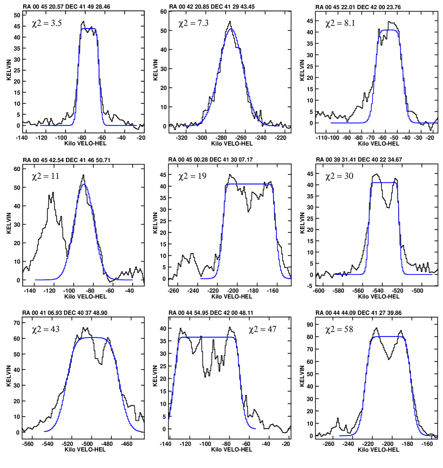
Figure 14: Illustration of spectral fits. Actual spectra at the positions indicated above each box with best-fitting models overlaid (smooth curves). The goodness-of-fit is indicated for each spectrum with the normalized $\chi^{2}$. Goodness of fit decreases from left-to-right and top-to-bottom, primarily due to the effects of velocity blending of physically unrelated features. A cut-off $\chi^{2}\sim 25$ was found to best distinguish blended from unblended spectra.

Plausible spectral fits were possible for most lines-of-sight. However, there are locations in the M31 disk where emission features which are likely at significantly different distances along the line-of-sight become strongly blended in velocity. Such circumstances are most apparent in position-velocity images made parallel to the major axis, in which continuous spiral arm segments can be tracked as linear features with approximately constant orientation (as documented by Braun (1991)). The gradient of velocity with major axis distance,

$${dV\over dX}={V_{c}(R)sin(i(R))\over R}$$ (4)

is proportional to the local projected rotation velocity divided by the radial distance of the feature within the galaxy. The ocurrence of apparently intersecting linear features in position-velocity plots is a strong indication for velocity blending of physically unrelated features which reside at different radii in the galaxy. The most prominent instances of such velocity overlap occur in four locations within M31 at major axis distances of both $\pm 30$ arcmin and minor axis distances of both $\pm 10$ arcmin.

The challenges of velocity blending are illustrated by the sequence of individual spectra with overlaid fits shown in Fig. 14. The sequence of spectra from left to right and top to bottom are ordered by decreasing quality of fit, as measured by the normalized $\chi^{2}=\Sigma_{i}(D_{i}-M_{i})^{2}/(N\sigma^{2})$. Our fitting method could deal successfully only with instances of sufficiently separated spectral features, where the local minima drop below 50% of the peak. More blended features are straddled with a single broad profile fit. From a careful examination of individual cases of blended and unblended profiles, based on the presence or absence of intersecting linear position-velocity features as described above, we established a cut-off in fit quality of $\chi^{2}=25$ that most effectively seperated these two regimes. Only those fits with a $\chi^{2}$ below this cut-off were retained, resulting in rejection of some 4% of the total. Concentrations of rejected fits are located in the expected regions (noted above).

The results of our spectral fitting were recorded as images of the physical parameters, $N_{HI}^{Fit},T_{S}$ and $\sigma_{NT}$ together with the integral of brightness temperature over velocity that corresponds to the column density of the fit, $\int T_{B}^{Fit}dV$. This allowed calculation of a total corrected column density image from,

$$N_{HI}^{Tot}=N_{HI}^{Fit}+1.823\times 10^{18}\biggl{(}\int T_{B}^{Tot}dV-\int T_{B}^{Fit}dV\biggr{)}$$ (5)

where $\int T_{B}^{Tot}dV$ is just the usual image of integrated emission. In this way any spectral component not accounted for by the fit to the peak was retained, albeit with the assumption of negligible opacity for this residual. Those lines-of-sight with insufficient fit quality ($\chi^{2}>25$) were assumed to have negligible opacity. The two column density images (assuming negligible optical depth and fitting for it) are contrasted in Figs. 15 and 16. Substantially more fine-scale structure is apparent in the opacity-corrected column density, primarily in the form of compact features and narrow filaments. The narrow filaments, in particular, correspond to those seen in the images of velocity coherence, shown in Figs. 6–8. Peak column densities are enhanced by about an order of magnitude over the uncorrected version.

Given the uncertainties in the fit parameters, we do not attach undue significance to each pixel in the images of corrected column density, since they may easily be in error by a factor of 2 or more, but are encouraged by the spatial continuity of the solutions, since the fit to every line-of-sight is carried out independently of all others. Some indication for the relevance of the fit results can be obtained by comparison with high signal-to-noise observations of H I absorption toward background continuum sources. As noted previously, several bright background continuum sources that have been studied by Braun & Walterbos (1992) fall fortuitously near regions of significant self-opacity, particularly the sources B0039+412 and B0044+419 for which peak optical depths of $\tau_{max}=0.46\pm 0.02$ and $\tau_{max}=1.06\pm 0.06$ are observed. (Note that $(1-e^{-\tau})$ rather than $\tau$ is tabulated in the reference.) The model fits show very substantial structure in the vicinity of these background sources, making it difficult to estimate the likely line-of-sight parameters. We have determined the average peak model opacity over a 3$\times$3 pixel region that is offset azimuthally from the direction of each of these sources by one beamwidth. For these two lines-of-sight this yields $\tau_{max}=0.4\pm 0.4$ and $\tau_{max}=1.1\pm 0.8$. Although the pixel-to-pixel variation is very large, and may well represent real structure rather than fitting errors, the order-of-magnitude of the opacity is estimated correctly in these cases.

The total detected H I mass of M31 is increased by the opacity corrections by about 30%, from 5.76$\times 10^{9}$ to 7.33$\times 10^{9}$ M_⊙. In view of the necessity of discarding all blended profiles, this should be regarded as a lower limit to the actual mass correction (within the limitations of our approach).

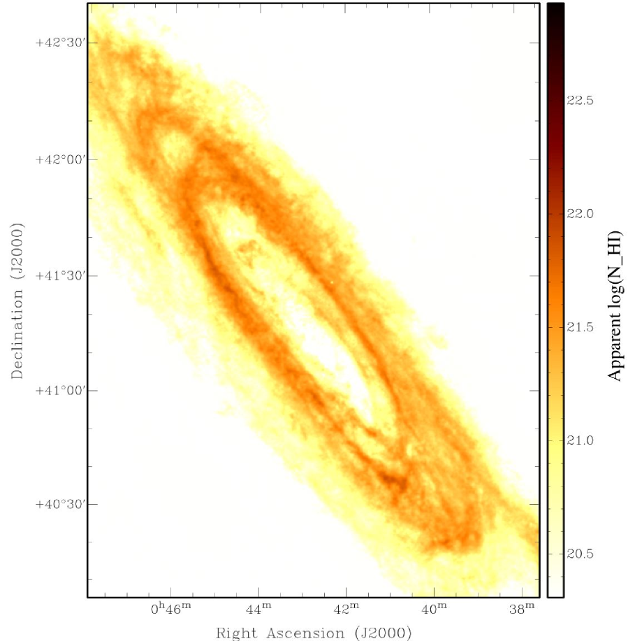
Figure 15: Column density of H I assuming negligible opacity of the central 25% of the survey region.

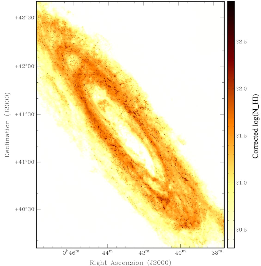
Figure 16: Column density of H I derived from a fit to each spectrum of the isothermal model described in §4.2 for the central 25% of the survey region.

The best-fit spin temperature and non-thermal velocity dispersion are shown in Figs. 17–18. Regions of significant opacity (log($N_{HI}$) $>$ 22) have spin temperatures of less than about 100 K and are often organized into patchy filamentary complexes. While there is some organized spatial structure in the distribution of non-thermal velocity dispersion, it is not obviously correlated with either the total column density or spin temperature. Not surprisingly, there is a significant correlation of the non-thermal velocity dispersion of the fits with the image of velocity coherence (shown in the right hand panels of Figs. 6–8).

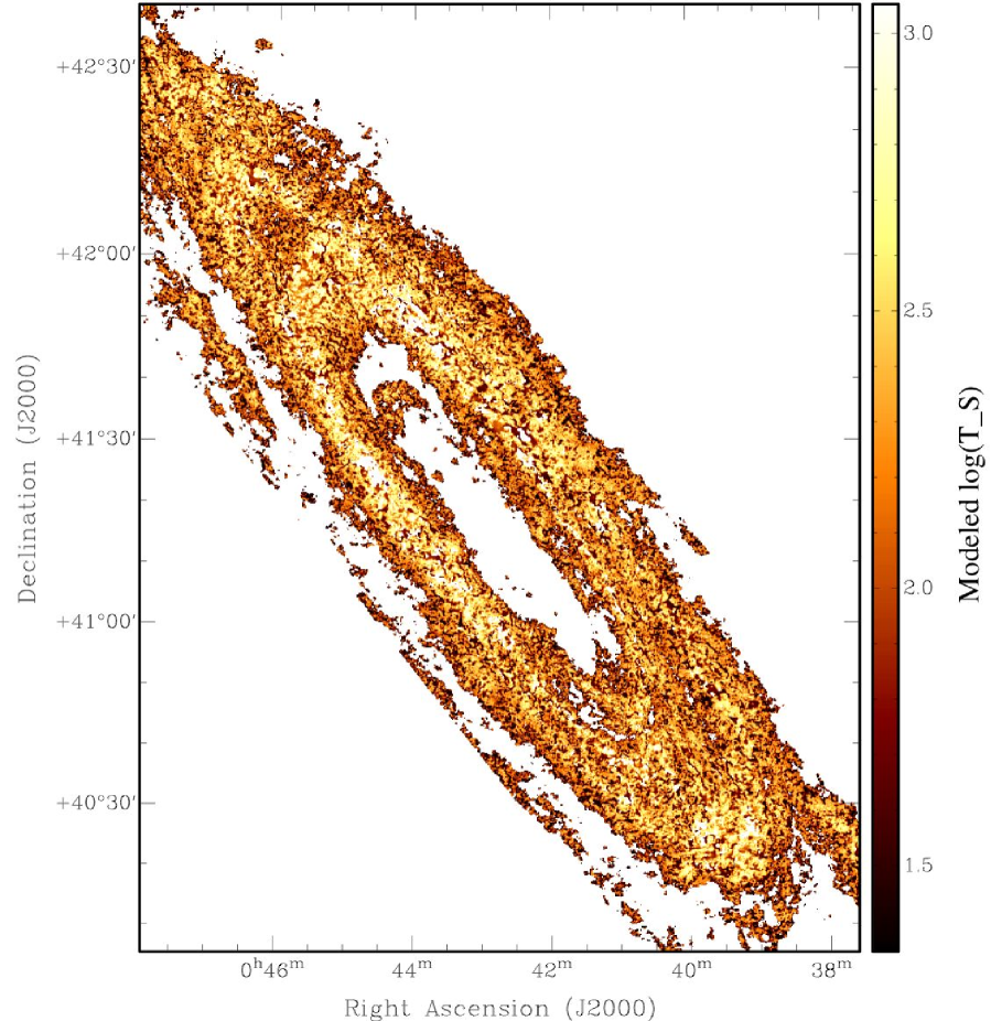
Figure 17: The logarithm of the spin temperature of H I derived from a fit to each spectrum of the isothermal model described in §4.2 for the central 25% of the survey region.

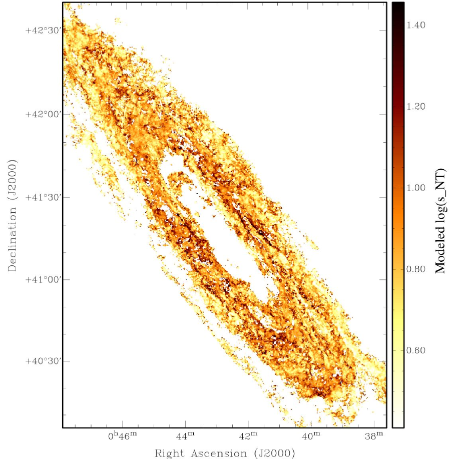
Figure 18: The logarithm of the non-thermal velocity dispersion of H I derived from a fit to each spectrum of the isothermal model described in §4.2 for the central 25% of the survey region.

4.3 Radial Trends

The basic radial trends of observed and derived quantities are illustrated in Fig. 19. The peak observed brightness temperature (Panel A) is seen to first increase dramatically with radius out to about 12 kpc and then subsequently to decline out to the the largest detected radii. Even the median peak brightness exceeds 50 K near 12 kpc, while the distribution extends out beyond 100 K. This can be compared with the very general trend documented by Braun (1997) for a positive gradient in peak brightness to occur within the actively star forming disk of nearby galaxies. The unprecented physical sensitivity obtained for M31 allows us to track the atomic gas properties out to more than three times larger radii. The apparent column density distribution in Panel B follows a similar trend, illustrating the exponential character of both the increase to- and the subsequent decline from- the peak near 12 kpc. A 6 kpc scale-length exponential function is overlaid on the plots in Panels B, C, D and H to illustrate how well this scale-length describes the gas mass density. Intriguingly, the old stellar population of M31, as traced by 3.6 $\mu$m Spitzer imaging between 1 and 12 kpc radius is best-fit with a 6.08$\pm$0.09 kpc scale-length exponential (Barmby et al., 2006). The corrected H I column density, shown in Panel C, has a median ridge-line that closely tracks the apparent column, but also demonstrates that outliers to higher corrected column occur primarily at radii between about 7 and 30 kpc. Adding in the molecular contribution to mass surface density (as described in detail in § 4.4) in Panel D yields only minor changes to the radial trend of the atomic column density. The most significant is a slight addition of mass density near 12 kpc, where the molecular contribution permits the total to better track the 6 kpc exponential to slightly smaller radii. Inside of about 12 kpc is a sharp cut-off that can be described with a 3 kpc exponential scale-length. Beyond about 28 kpc, where opaque H I is no longer found, there is a significant truncation of the disk exponential (neutral) mass density, corresponding to a 2 kpc scale-length. The corresponding face-on column density (scaled by 1/cos(78^∘)) where this outer truncation sets in, is 5$\times 10^{19}$cm^-2.

The radial distribution of velocity coherence (Panel E) shows a similar trend, rising rapidly out to about 10 kpc, then declining out to about 30 kpc and then plummeting. Both the derived non-thermal velocity dispersion (Panel F) and spin temperature (Panel G) show some broad systematic decline with radius beyond 10 kpc. For the spin temperature, it is only the lower envelope of the distribution which represents “opaque” fits. These “opaque” cool component temperatures are as low as 20 K near 7 and 25 kpc, but increase to about 60 K near 10 kpc. This is quite distinct from the most highly populated ridge-line, which represents predominantly “transparent” lines-of-sight. The ridge-line shows a similar trend, but is offset to higher temperatures by about an order of magnitude. Current massive SFR density (as defined below in § 4.4) is shown in Panel H. The apparent nuclear peak in SFR density is due to other processes (as discussed below), while current coverage only extends to about 20 kpc. Current SFR density is highly peaked near 12 kpc, where gas mass densities are highest and does not track the 6 kpc exponential of the median gass mass density.

4.4 The Surface Density of Gas Mass and Star Formation Rate

A particular form of correlation of observable parameters deserves special consideration, namely that between the surface density of gas mass and the star formation rate. Many authors have addressed the relationship between these properties on both a global and local level, beginning with the pioneering study of Schmidt (1959) and most recently by Kennicutt et al. (2007) and Thilker et al. (2007), who probe the resolved relationship of these parameters down to scales of 500 pc within NGC 5194 (M51a) and 400 pc within NGC 7331 respectively. Given the proximity of M31 we can extend this work by more than an order of magnitude to smaller surface area at spatial scales of 100 pc, albeit with a substantial inclination correction that introduces some potential linear smearing (by a factor of 4.8) in one dimension. Mass and star formation rates have been calculated after background subtraction and spatial smoothing of all relevant images to the same 30 arcsec (113 pc) Gaussian resolution as applies to the H I properties.

The mass surface density was calculated from the integrated CO(1–0) emission observed with the IRAM telescope by Nieten et al. (2006) assuming a mean atomic mass of 1.36 m_H and an N${}_{H_{2}}$/I_CO conversion factor of 2.8$\times 10^{20}$cm^-2/K-km s^-1. This differs from the procedure adopted by Kennicutt et al. (2007), (hereafter K07) who keep the comparison in terms of hydrogen nuclei (rather than including a Helium mass correction). The helium mass correction amounts to a shift by +0.13 dex in mass density. Note that the CO data only extend over the central 2$\times$0.5 degrees (or 28$\times$32 deprojected kpc in diameter). Radii beyond about 15–20 kpc therefore only have an H I contribution to the calculated mass density. Although the CO brightness at the edges of the sampled region is generally faint and has a low surface covering factor, isolated pockets of CO may well be present at larger radii.

The star formation density was calculated following the methodology of Thilker et al. (2007) from the Spitzer IRAC 8$\mu$m and MIPS 24$\mu$m surface brightness of Gordon et al. (2006) together with the GALEX FUV image of Thilker et al. (2005) and Gil de Paz et al. (2007). The “bolometric” luminosity was assumed to be, $L(bol)=\nu_{FUV}L_{\nu,obs}(FUV)+(1-\eta)L(IR)$ after correcting the FUV image for foreground extinction by the Galaxy, and assuming $\eta$=0.32. The term “bolometric” in this context is a misnomer, since the quantity is not assumed to represent a true integral of the entire SED, but merely to provide sensitivity to both directly emitted UV and re-radiated IR light. The value of $\eta$, which represents the fraction of the IR luminosity due to an older stellar population, is expected to vary substantially with environment within a galaxy. Ideally, this would also be modeled in a position dependent way, but that is beyond the scope of the current discussion.

The total (3-1100um) IR luminosity per pixel was estimated using the IRAC/MIPS data and the relation,

$$log\bigg{[}{L(IR)\over\nu L_{\nu}(24\mu m)}\bigg{]}=1.06+0.475\ log\bigg{[}{F_{\nu}(8\mu m)\over F_{\nu}(24\mu m)}\bigg{]}$$ (6)

and then converted to a star formation rate density using the projected pixel area and the SFR calibration:

$$log\ SFR(bol)(M_{\odot}yr^{-1})=log\ L(bol)(L_{\odot})-9.75.$$ (7)

The 24$\mu$m data only extend over the brighter disk region of $\sim$3$\times$1 degrees.

Only pixels with significant emission in the spatially smoothed images were used for the comparison, which resulted in thresholds at a brightness of 0.7 K-km s^-1 for the CO emission, H I columns greater than 19 in the log and sky-subtracted IR brightness greater than 0.06 MJy/sr at 24$\mu$m and 0.1 MJy/sr at 8$\mu$m. As can be seen in Fig. 19, the spatial coverage and sensitivity in the IR only extends out to a radius of about 20 kpc.

We contrast three different versions of the star formation law in Fig. 20 utilizing the molecular only, the molecular plus apparent H I and the molecular plus opacity-corrected H I column density. The molecular-only plots are overplotted both the relation of K07 with slope 1.37, a value which has also been found by Heyer et al. (2004) in M33, as well as a line with unit slope corresponding to a constant gas depletion time-scale, as advocated by Wong & Blitz (2002), (hereafter WB02). The slope of the molecular-only relationship is approximately matched by the simple linear dependency. The gas depletion time-scale of the plotted line is 1 Gyr (for a N${}_{H_{2}}$/I_CO conversion factor of 2$\times 10^{20}$cm^-2/K-km s^-1 as assumed by Wong & Blitz). This is similar to many of the galaxies analyzed in WB02, although occurring at mass and star formation densities that are at least an order of magnitude lower within M31. The M51a molecular-only relation of K07 is both steeper and shifted to higher mass densities by at least 0.3 dex.

The total-gas mass density plots are over-plotted with the relation fit by K07 to the M51a data with slope 1.56. Note that we have plotted star formation rate density in units of M_⊙pc^-2Gyr^-1 rather than the M_⊙kpc^-2yr^-1 of K07 implying a shift of 3 dex. The different units of both axes (relative to K07) have been taken into account for the overplotted curves. Remarkably, the M51a relation provides a very good fit to the M31 data, despite the fact that it has been derived in the strongly molecular-dominated inner disk of M51 and is being applied thoughout the atomic-dominated disk of M31. The highest contours of correlation probability are about twice as narrow for the total-gas relation compared to the molecular-only one. In the relation using apparent H I, there is a very steep truncation to mass densities exceeding about 10 M_⊙pc^-2, together with a saturation that sets in near 16 M_⊙pc^-2. This truncation disappears in the opacity-corrected H I relation, together with a small shift of the peak correlation ridge-line to higher mass densities. The saturation effect near 16 M_⊙pc^-2, is also alleviated although not entirely eliminated.

Data at the smallest radii ($<$5 kpc) yield the diffuse region of elevated apparent  star formation in the total gas panels of the figure. The enhanced 24$\mu$m emission from the nuclear regions of M31 is accompanied by both recombination- and forbidden emission line gas (as first documented by Jacoby et al. (1985)) with line ratios suggestive of shock heating, and as such is not due to massive star formation. Essentially no CO is detected from the nuclear region, so this feature is not apparent in Panels A and D. Beyond about 5 kpc, the same basic correlation is seen to apply at all radii, with only the range of the observables showing some systematic variation, but not the basic ridge-line of their correlation. The sharp truncation of the molecular-only mass density near 1 M_⊙pc^-2 is a consequence of the limited sensitivity. The same is true for star formation rate densities below about 0.2 M_⊙pc^-2Gyr^-1.

At star formation rate densities below about 0.4 M_⊙pc^-2Gyr^-1 and total gas surface densities of about 5 M_⊙pc^-2 there appears to be a departure from the power-law relationship. The same feature can be seen in the NGC 7331 data of Thilker et al. (2007) at a similar location, although this is near the noise floor in both cases. This may indeed be a distinct threshold for the formation of molecular clouds from which stars will form. The most substantial contribution to this possible threshold comes from radii in excess of 15 kpc.

Perhaps the most surprising aspect of Fig. 20 is the good statistical correlation of total gas mass and star formation density down to spatial scales of about 100 pc and gas masses of only 5$\cdot 10^{4}$ M_⊙, well inside the regime of individual, giant molecular clouds.

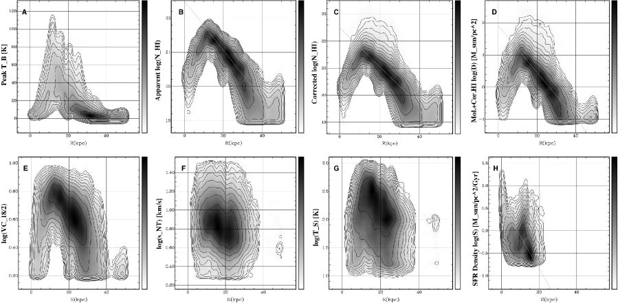
Figure 19: The radial distribution of several diagnostic properties of M31. The plotted quantities are the peak H I brightness temperature, apparent H I column density, corrected H I column density, the face-on gas mass surface density in M_⊙pc^-2, H I velocity coherence, the best-fit non-thermal velocity dispersion (labelled log(s_NT)) the best-fit cool H I temperature (labelled log(T_S)) and the estimated face-on star formation rate density in M_⊙pc^-2Gyr^-1 based on FIR and UV surface brightness. Note that the central peak in panel H is not due to star formation (see text). Contours are drawn at factors of two in correlation density beginning at 0.1% and ending at 51%. The greyscale extends from 0 and 100% with a square-root transfer function. The gray solid line in panels B, C, D and H is an exponential with 6.0 kpc scale-length.

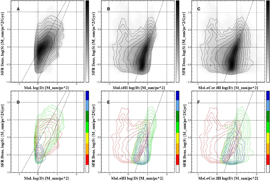
Figure 20: Star formation rate density versus gas mass density in M31. The face-on gas mass surface density has units of M_⊙pc^-2 and the face-on star formation rate density, M_⊙pc^-2Gyr^-1. The mass surface density is calculated with molecular only–, molecular plus apparent H I– and molecular plus opacity-corrected H I column density from left to right. The data at all radii are shown on the top, while the radially binned data is shown on the bottom. Contours are drawn at factors of two in correlation density beginning at 0.5% and ending at 64%. The greyscale extends from 0 and 100% with a square-root transfer function. The colors red, green and blue correspond to bins in galactocentric radius of 0–8, 8–16 and 16–24 kpc. The diagonal lines of slope 1.37 (molecular only) and slope 1.56 (molecular plus atomic) are the relations given in Kennicutt et al. (2007). A second line of unit slope is plotted in the molecular-only plots, corresponding to a gas depletion timescale of 1 Gyr.

5 Conclusions

Our high resolution and signal-to-noise study of the neutral ISM of M31 has permitted a number of novel results:

1. We detect ubiquitous self-opaque H I features, discernible in the first instance as filamentary local minima in images of the peak H I brightness temperature. Such local minima are often accompanied by systematically broader line profiles, apparent in images of the velocity coherence. High opacity features are organized into complexes of more than kpc length and are particularly associated with the leading edge of spiral arms. We suggest that such features are the counterpart of large-scale H I self-absorption (HISA) features seen in the Galaxy. They are the consequence of a “sandwich” geometry of two warm, semi-opaque layers which flank a colder, opaque core. Such a geometry leads to widespread HISA in the edge-on Galactic disk, but is spatially resolved into distinct parallel filaments in the inclined disk of M31. Just as in the Galaxy, there is only patchy correspondence of self-opaque/HISA features with CO(1-0) emission.

2. We have produced images of the best-fit physical parameters; spin temperature, opacity-corrected column density and non-thermal velocity dispersion, for the brightest spectral feature along each line-of-sight in the M31 disk. This represents a major step forward in the quantitative assessment of H I opacity in a galactic context. Opaque atomic gas is organized into filamentary complexes and isolated clouds down to the resolution limit of 100 pc. The spin temperature of opaque regions first increases systematically with radius from about 20 to 60 K (for radii of 5 to 12 kpc) and then smoothly declines again to 20 K by about 25 kpc. Opacity corrections to the column density exceed an order of magnitude in many cases and add globally to a 30% increase in the atomic gas mass over that inferred from the integrated brightness under the usual assumption of negligible self-opacity. It will be particularly interesting to undertake a similar analysis of more nearly face-on systems like M33 and the LMC, where spectral blending will be even less of an issue.

3. We have constructed the radial distribution of gas mass density which illustrates a remarkably extended exponential decline with 6 kpc scale-length between 12 and 28 kpc. Inside of 12 kpc there is a rapid decline in neutral mass density with 3 kpc scale-length, while beyond 28 kpc at a face-on column density of 5$\times 10^{19}$cm^-2 is a truncation of the atomic disk with 2 kpc scale-length. Perhaps fortuitously, the extended disk scale-length of 6 kpc matches that of the old stellar population traced by 3.6 $\mu$m emission.

4. We have extended the resolved correlation of star-formation-rate- with gas-mass-density down to the smallest physical scales yet reached, of only 100 pc and $10^{4}$ M_⊙; more than an order of magnitude smaller in area and mass than has been possible previously. Unlike other galaxies, in which the gas mass is dominated by molecular gas as traced by CO emission at small radii, M31 is dominated by atomic gas at all radii. The relation of molecular-mass- to star-formation-density has a large dispersion, but has a slope near unity and a corresponding gas depletion timescale of about 1 Gyr, similar to many galaxies studied by Wong & Blitz (2002). The relation between total-gas-mass- and star-formation-rate-density is significantly tighter and is fully consistent in both slope and normalization  with the relation found in the molecule-dominated disk of M51 by Kennicutt et al. (2007) at 500 pc resolution. Together, the M31 and M51 data demonstrate the same relationship spanning mass-densities from about 5 to 700 M_⊙pc^-2. Use of opacity-corrected H I columns yields a more symmetric distribution with less evidence of truncation effects than with the apparent H I column. Below about 5 M_⊙pc^-2, there is a down-turn in star-formation-density which may represent a real local threshold for massive star formation. The corresponding threshold cloud mass is about 5$\cdot 10^{4}$ M_⊙.

References

- Barmby et al. (2006) Barmby, P., Ashby, M.L.N., Bianchi, L. et al., 2006, ApJL, 650, L45
- Braun (1991) Braun, R., 1991, ApJ, 372, 54
- Braun & Walterbos (1992) Braun, R., Walterbos, R.A.M, 1992, ApJ, 386, 120
- Braun (1995) Braun, R., 1995, A&AS, 114, 409
- Braun (1997) Braun, R., 1997, ApJ, 484, 637
- Braun & Thilker (2004) Braun, R., Thilker, D.A., 2004, A&A, 417, 421
- Braun & Kanekar (2005) Braun, R., Kanekar, N., 2005, A&A, 436, L53
- Brinks & Shane (1984) Brinks, E., Shane, W.W., 1984, A&AS, 55, 179
- Carignan et al. (2006) Carignan, C., Chemin, L., Huchtmeier, W.K., Lockman, F.J., 2006, ApJ, 641, L109
- Davies (1975) Davies, R.D., 1975, MNRAS, 170, 45
- De Heij et al. (2002) de Heij, V., Braun, R., Burton, W.B., 2002, A&A, 391, 67
- Van de Hulst et al. (1957) van de Hulst, H.C, Raimond, E., van Woerden, H., 1957, BAN, 14, 1
- Gibson et al. (2000) Gibson, S.J., Taylor, A.R., Higgs, L.A., Dewdney, P.E., 2005, ApJ, 540, 851
- Gibson et al. (2005) Gibson, S.J., Taylor, A.R., Higgs, L.A. et al., 2005, ApJ, 626, 195
- Gil de Paz et al. (2007) Gil de Paz, A., Boissier, S, Madore, B.F., et al. 2007, ApJS, 173, 185
- Goldsmith & Li (2005) Goldsmith, P.F., Li, D., 2005, ApJ, 622, 938
- Gooch (1996) Gooch, R., 1996, ASP Conf. Ser. 101, 80
- Gordon et al. (2006) Gordon, K.D., Bailin, J., Engelbracht, C.W., et al. 2006, ApJ, 638, L87
- Henderson et al. (1982) Henderson, A.P., Jackson, P.D., Kerr, F.J., 1982, ApJ, 263, 116
- Heyer et al. (2004) Heyer, M.H., Corbelli, E., Schneider, S.E., Young, J.S., 2004, ApJ, 602, 723
- Jacoby et al. (1985) Jacoby, G.H., Ford, H., Ciardullo, R., 1985, ApJ, 290, 136.
- Kalberla et al. (2005) Kalberla, P.M.W., Burton, W.B., Hartmann, D., et al. 2005, A&A, 440, 775
- Kennicutt et al. (2007) Kennicutt, R.C., Calzetti, D., Walter, F. et al. 2007, ApJ, 671, 333
- Kim et al. (2003) Kim, S., Staveley-Smith, L., Dopita, M.A., et al. 2003, ApJS, 148, 473
- Liszt (2001) Liszt, H., 2001, A&A, 371, 698
- Marius (1612) Marius, S., 1612, Mundus Jovialis
- McConnachie et al. (2005) McConnachie, A.W., Irwin, M.J., Ferguson, A.M.N., et al. 2005, MNRAS, 356, 979.
- Nieten et al. (2006) Nieten, Ch., Neininger, N., Guelin, M. et al. 2006, A&A, 453, 459
- Popping & Braun (2008) Popping, A., Braun, R., 2008, A&A, 479, 903
- Radhakrshnan (1960) Radhakrishnan, V., 1960, PASP, 72, 427
- Rohlfs et al. (1972) Rohlfs, K., Braunsfurth, E., Mebold, U. 1972, AJ, 77, 711
- Sault et al. (1995) Sault, R.J., Teuben, P.J., Wright, M.C.H., 1995, ASP Conf.Ser., 77, 433
- Schmidt (1957) Schmidt, M., 1957, Bull.Astron.Inst.Netherlands, 13, 247
- Schmidt (1959) Schmidt, M., 1959, ApJ, 129, 243
- Thilker et al. (2004) Thilker, D.A., Braun, R., Walterbos, R.A.M. et al., 2004, ApJL, 601, 39
- Thilker et al. (2005) Thilker, D.A., Hoopes, C., Bianchi, L. et al. 2005, ApJ, 619, L67
- Thilker et al. (2007) Thilker, D.A., Boissier, S., Bianchi, L. et al. 2007, ApJS, 173, 572
- Unwin (1983) Unwin, S.C., 1983, MNRAS, 205, 787
- Vilardell (2007) Vilardell, F., Ribas, I., Jordi, C., 2007, A&A, 473, 847
- Westmeier et al. (2005) Westmeier, T., Braun, R., Thilker, D.A., 2005, A&A, 436, 101
- Wong & Blitz (2002) Wong, T., Blitz, L., 2002, ApJ, 569, 157