Recovery of free energy branches in single molecule experiments

Abstract

We present a method for determining the free energy of coexisting states from irreversible work measurements. Our approach is based on a fluctuation relation that is valid for dissipative transformations in partially equilibrated systems. To illustrate the validity and usefulness of the approach, we use optical tweezers to determine the free energy branches of the native and unfolded states of a two-state molecule as a function of the pulling control parameter. We determine, within $0.6\ k_{\rm B}T$ accuracy, the transition point where the free energies of the native and the unfolded states are equal.

Recent developments in statistical physics Jarzynski:1997yh have provided new methods to extract equilibrium free energy differences in small systems from measurements of the mechanical work in irreversible processes (see kurchan:2007uh ; ritort:2008ik for reviews). In this regard, fluctuation relations kurchan:2007uh are generic identities that establish symmetry properties for the probability of exchanging a given amount of energy between the system and its environment along irreversible processes. If a system, initially in thermodynamic equilibrium, is strongly perturbed by fast varying a control parameter $\lambda$ between two values $\lambda_{0}$ and $\lambda_{1}$, then the system is driven out of equilibrium. The work exerted upon the system, averaged over the ensemble of all possible trajectories, reads $\langle W\rangle=\langle\int_{\lambda_{0}}^{\lambda_{1}}\;(\partial{\cal H}/\partial\lambda)d\lambda\rangle$ where ${\cal H}$ is the system Hamiltonian. According to the second law of thermodynamics, $\langle W\rangle$ is always greater than the free energy difference between the initial and final states, $\Delta G=G(\lambda_{1})-G(\lambda_{0})$. The Crooks fluctuation relation Crooks:2000ez extends the predictive power of the Second Law by establishing a symmetry relation for arbitrary functionals of a trajectory $\Gamma$ measured along a nonequilibrium process (forward or F process) and its time reversed one (reverse or R process). In the forward process the system starts in equilibrium at $\lambda_{0}$ and $\lambda$ is varied from $\lambda_{0}$ to $\lambda_{1}$ for a time $t_{f}$ according to an arbitrary protocol $\lambda(t)$ (i.e., $\lambda_{1}=\lambda(t_{f})$). In the reverse process the system starts in equilibrium at $\lambda_{1}$ and $\lambda$ is varied from $\lambda_{1}$ to $\lambda_{0}$ following the time reversed scheme, given by $\lambda(t_{f}-t)$. In its most general form the Crooks fluctuation relation reads Crooks:2000ez

$$\langle\mathcal{F}\exp[-\beta(W-\Delta G)]\rangle_{\mathrm{F}}=\langle\hat{\mathcal{F}}\rangle_{\mathrm{R}}\,,$$ (1)

where $\mathcal{F}$ stands for an arbitrary functional of the forward trajectories the system can take through phase space, $\beta$ is the inverse of the thermal energy $k_{\mathrm{B}}T$ where $k_{\mathrm{B}}$ is the Boltzmann constant and $T$ the temperature of the environment. In this relation, $\hat{\mathcal{F}}$ is the time reversal of $\mathcal{F}$, while the averages $\langle\bullet\rangle_{\mathrm{F}(\mathrm{R})}$ are taken over the ensemble of all possible forward (reverse) trajectories. The particular case $\mathcal{F}=\delta(W-W(\Gamma))$ yields a relation between work distributions along the forward and reverse processes, $P_{\mathrm{F}}(W)=P_{\mathrm{R}}(-W)\exp[\beta(W-\Delta G)]$. This relation has been experimentally tested and used to extract free energy differences in single molecule experiments Hummer:2001 ; Collin:2005rb ; Imparato:2008 . A thorough discussion on its validity domain can be found in Crooks:2000ez

Fluctuation relation under partial equilibrium conditions.

By considering only the trajectories that go from one specific subset of configurations to another one, Maragakis et al. Maragakis:2008hj have derived another relation useful to extract free energy differences between subsets of states. In principle, the validity of Eq. (1) is restricted to initial conditions that are Gibbsian over the whole phase space $\mathcal{S}$ (what we might call global thermodynamic equilibrium). It is, however, possible to extend Eq. (1) to the case where the initial state is Gibbsian but restricted over a subset of configurations (what we might call partial thermodynamic equilibrium). A relation mathematically similar to Eq. (1) can be derived, but involving nonequilibrium processes that are in partial (rather than global) equilibrium. It is useful to rephrase here the derivation in such a way to emphasize the role played by partial equilibrium. As we will see this makes it possible to experimentally determine the free energy of coexisting states for values of $\lambda$ such that the system is never globally equilibrated.

Let $P_{\lambda,\mathcal{S^{\prime}}}^{\rm eq}({\cal C})$ denote the partially equilibrated (i.e., Boltzmann–Gibbs) distribution for a given value of $\lambda$. Such distribution is restricted over a subset $\mathcal{S^{\prime}}$ of configurations ${\cal C}$ contained in $\mathcal{S}$ (i.e., ${\cal C}\in\mathcal{S^{\prime}}\subseteq\mathcal{S}$). The case $\mathcal{S^{\prime}}=\mathcal{S}$ corresponds to global equilibrium: $P_{\lambda}^{\rm EQ}({\cal C})\equiv P^{\rm eq}_{\lambda,\mathcal{S}}({\cal C})$. Partially equilibrated states satisfy $P^{\rm eq}_{\lambda,\mathcal{S^{\prime}}}({\cal C})=P^{\rm EQ}_{\lambda}({\cal C})\chi_{\mathcal{S^{\prime}}}({\cal C}){\cal Z}_{\lambda,\mathcal{S}}/{\cal Z}_{\lambda,\mathcal{S^{\prime}}}$, where $\chi_{\mathcal{S^{\prime}}}$ is the characteristic function defined over the subset $\mathcal{S^{\prime}}$ ($\chi_{\mathcal{S^{\prime}}}({\cal C})=1$ if ${\cal C}\in\mathcal{S^{\prime}}$ and zero otherwise), and ${\cal Z}_{\lambda,\mathcal{S^{\prime}}}$ is the partition function restricted to the subset $\mathcal{S^{\prime}}$, i.e., ${\cal Z}_{\lambda,\mathcal{S^{\prime}}}=\sum_{{\cal C}\in\mathcal{S^{\prime}}}\exp(-\beta E_{\lambda}({\cal C}))$, with $E_{\lambda}({\cal C)}$ the energy function of the system for a given $\lambda$ and ${\cal C}$. Given a forward trajectory $\Gamma$, going from configuration ${\cal C}_{0}$ when $\lambda=\lambda_{0}$ to ${\cal C}_{1}$ for $\lambda=\lambda_{1}$, let ${\cal S}_{0}$ (${\cal S}_{1}$) be the subset of ${\cal S}$ over which the system is partially equilibrated at $\lambda_{0}$ ($\lambda_{1}$). Consider now the following transformation of the functional $\mathcal{F}$ in Eq. (1): $\mathcal{F}(\Gamma)\to\chi_{\mathcal{S}_{0}}(\mathcal{C}_{0})\mathcal{F}(\Gamma)\chi_{\mathcal{S}_{1}}(\mathcal{C}_{1})$. Under previous conditions the following identity can be proved (see Supp. Mat.):

$$\frac{\langle\mathcal{F}\exp[-\beta(W-\Delta G_{\mathcal{S}_{0},\lambda_{0}}^{\mathcal{S}_{1},\lambda_{1}})]\rangle_{\mathrm{F}}^{\mathcal{S}_{0}\to\mathcal{S}_{1}}}{\langle\hat{\mathcal{F}}\rangle_{\mathrm{R}}^{\mathcal{S}_{0}\leftarrow\mathcal{S}_{1}}}=\frac{p_{\mathrm{R}}^{{\cal S}_{0}\leftarrow{\cal S}_{1}}}{p_{\mathrm{F}}^{{\cal S}_{0}\to{\cal S}_{1}}}\,,$$ (2)

where the average $\langle\bullet\rangle^{\mathcal{S}_{0}\to\mathcal{S}_{1}(\mathcal{S}_{0}\leftarrow\mathcal{S}_{1})}_{\mathrm{F}(\mathrm{R})}$ is now restricted to forward (reverse) trajectories that start in partially equilibrated state $\mathcal{S}_{0}$ ($\mathcal{S}_{1}$) at $\lambda_{0}$ ($\lambda_{1}$) and end in $\mathcal{S}_{1}$ ($\mathcal{S}_{0}$) at $\lambda_{1}$ ($\lambda_{0}$). $p_{\mathrm{F}}^{{\cal S}_{0}\to{\cal S}_{1}}$ ($p_{\mathrm{R}}^{S_{0}\leftarrow S_{1}}$) stands for the probability to be in ${\cal S}_{1}$ (${\cal S}_{0}$) at the end of the forward (reverse) process defined above, and $\Delta G_{\mathcal{S}_{0},\lambda_{0}}^{\mathcal{S}_{1},\lambda_{1}}=G_{\mathcal{S}_{1}}(\lambda_{1})-G_{\mathcal{S}_{0}}(\lambda_{0})$ is the free energy difference between partially equilibrated states $\mathcal{S}_{0}$ and $\mathcal{S}_{1}$. In the following, we will drop the subscript (F, R), leaving the direction of the arrow to distinguish forward from reverse. Moreover, we will adopt the shorthand notation $\mathcal{P}_{{\cal S}_{0}}^{{\cal S}_{1}}\equiv p^{{\cal S}_{0}\to{\cal S}_{1}}/p^{{\cal S}_{0}\leftarrow{\cal S}_{1}}$. If $\mathcal{F}=1$ we obtain a generalization of the Jarzynski equality, $\mathcal{P}_{{\cal S}_{0}}^{{\cal S}_{1}}\langle\exp[-\beta(W-\Delta G_{\mathcal{S}_{0},\lambda_{0}}^{\mathcal{S}_{1},\lambda_{1}})]\rangle=1$. Whereas for the particular case $\mathcal{F}=\delta(W-W(\Gamma))$, we get the relation

$$\mathcal{P}_{{\cal S}_{0}}^{{\cal S}_{1}}\frac{P^{{\cal S}_{0}\to{\cal S}_{1}}(W)}{P^{{\cal S}_{0}\leftarrow{\cal S}_{1}}(-W)}=\exp[\beta(W-\Delta G_{\mathcal{S}_{0},\lambda_{0}}^{\mathcal{S}_{1},\lambda_{1}})]\,,$$ (3)

which has been used in Maragakis:2008hj in the case of global equilibrium initial conditions.

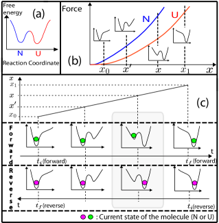
Figure 1: A two-state molecule in a pulling experiment. (a) Schematic picture of the free energy landscape in a two-state folder as a function of the reaction coordinate. The blue and red colors represent the subsets of configurations that define the $N$ and $U$ states respectively. (b) Depending on the value of the control parameter $x$, the shape of the free energy landscape is tilted toward one state (either $N$ or $U$). For each value of $x$, the Boltzmann–Gibbs equilibrium value of the force restricted to each state defines the native (blue) and unfolded (red) force-distance branches. (c) During a ramping protocol, $x$ is changed at a constant pulling speed from $x_{0}$ to $x_{1}$ (from $x_{1}$ to $x_{0}$ in the reverse case) and the molecule can visit both states as indicated by the colored circles. In order to measure $G_{U}(x)$ (all free energies are computed with respect to $G_{N}(x_{0})$) at a given value of $x$ (gray area), only forward and reverse trajectories that are in $N$ at $x_{0}$ and in $U$ at $x$ have to be considered (which is true only for the reverse trajectory in the example shown in the picture).

Experimental test.

Here we test the validity of Eq. (3) by performing single molecule experiments using optical tweezers. Let us consider an experiment where force is applied to the ends of a DNA hairpin that unfolds/refolds in a two-state manner. The conformation of the hairpin can be characterized by two states, the unfolded state ($U$) and the native or folded state ($N$) — see Fig. 1. The thermodynamic state of the molecule can be controlled by moving the position of the optical trap relative to a pipette (Fig. 2, upper panel). The relative position of the trap along the $x$-axis defines the control parameter in our experiments, $\lambda=x$. Depending on the value of $x$ the molecule switches between the two states according to a rate that is a function of the instantaneous force applied to the molecule Evans:1997np . In a ramping protocol the value of $x$ is changed at constant pulling speed from an initial value $x_{0}$ (where the molecule is always folded) to a final value $x_{1}$ (where the molecule is always unfolded) and the force $f$ (measured by the optical trap) versus distance $x$ curves recorded. By computing i) the fraction of forward trajectories (i.e., increasing $x$) that go from $N$ ($\equiv{\cal S}_{0}$) at $x_{0}$ to $U$ ($\equiv{\cal S}_{1}$) at $x$ and ii) the fraction of reverse trajectories (decreasing extension) that go from $U$ at $x$ to $N$ at $x_{0}$, we can determine $\mathcal{P}_{N}^{U}$. Then by measuring the corresponding work values for each of these trajectories, we can use Eq. (3) to estimate the free energy of the unfolded branch $G_{U}(x)$ as a function of $x$. By repeating the same operation with $N$ instead of $U$, the free energy of the folded branch $G_{N}(x)$ can be measured as well. Note that we adopt the convention of measuring all free energies with respect to the free energy $G_{N}(x_{0})$ of the native state at $x_{0}$. We are also able to compute the free energy difference between the two branches, $\Delta G_{N}^{U}(x)=G_{U}(x)-G_{N}(x)$.

We have pulled a 20 bps DNA hairpin using a miniaturized dual-beam laser optical tweezers apparatus hairpin . Molecules have been pulled at two low pulling speeds (40 and 50 nm/s) and two fast pulling speeds (300 and 400 nm/s), corresponding to average loading rates ranging between 2.6 and 26 pN/s, from $x_{0}=0$ to $x_{1}=110.26$ nm (for convenience we take the initial value of the relative distance trap-pipette equal to 0). A few representative force-distance curves are shown in Fig. 2 (inset of lower panel). We have then selected a value $x=\bar{x}=61.75$ nm, close to the expected coexistence value of $x$ where both $N$ and $U$ states have the same free energy (see below). Such value of $x$ is chosen in order to have good statistics for the evaluation of the unfolding and refolding work distributions. The system is out of equilibrium at the four pulling speeds. To extract the free energy of the unfolded branch $G_{U}(\bar{x})$, we have measured the work values $W^{N\to U}=\int_{x_{0}}^{\bar{x}}fdx$, $W^{N\leftarrow U}=\int_{\bar{x}}^{x_{0}}fdx$ along the unfolding and refolding trajectories, respectively, and then determined the distributions $P^{N\to U}(W)$ and $P^{N\leftarrow U}(-W)$. In the main panel of Fig. 2 we show the work distributions obtained for a slow and fast pulling process. Note that the support of the unfolding work distributions is bounded by the maximum amount of work that can be exerted on a molecule between $x_{0}$ and $\bar{x}$. This bound corresponds to the work of those unfolding trajectories that have never unfolded before reaching $\bar{x}$.

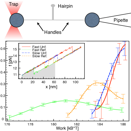
Figure 2: (Upper panel) Experimental setup. (Lower panel) Unfolding and refolding work distributions $P^{N\to U}(W)$, $P^{N\leftarrow U}(-W)$ at $x=\bar{x}=61.75$ nm measured at two pulling speeds: 300 nm/s (red -unfolding- and green -refolding-) and 40 nm/s (blue -unfolding- and orange -refolding-). In the inset we show two force-distance cycles corresponding to low (40 nm/s) and fast (300 nm/s) pulling speeds. The gray area indicates the mechanical work ($=\int_{\bar{x}}^{x_{0}}fdx$) exerted along the green refolding trajectory. Statistics (number of molecules, total number of unfolding/refolding cycles): 40 nm/s (2, 223), 50 nm/s (2, 183), 300 nm/s (3, 337), 400 nm/s (1, 551). More details about the data analysis procedure can be found in the Supp. Mat.

As a direct test of the validity of Eq. (3), in the upper panel of Fig. 3 we plot the quantity $\log(P^{N\to U}(W)/P^{N\leftarrow U}(-W))+\log\mathcal{P}^{U}_{N}(\bar{x})$ against $W$ (in $k_{\mathrm{B}}T$ units). As expected, all data fall into straight lines of slope close to 1. The intersections of such lines with the $W$-axis provide an estimate of $G_{U}(\bar{x})$. Note that both fast and slow pulling speeds intercept the horizontal axis around the same value within 0.75 $k_{\mathrm{B}}T$ of error. With this method, we estimate $G_{U}(\bar{x})=185.9(5)\ k_{\mathrm{B}}T$. Note that this free energy estimate, as all the others in this paper, refers to the whole system, comprising hairpin, handles, and trap.

Figure 3: Experimental verification of the fluctuation relation Eq. (3). (Upper panel) Plot of $\log\mathcal{P}^{U}_{N}(\bar{x})+\log(P^{N\to U}(W)/P^{N\leftarrow U}(-W))$ as a function of $W$ (in $k_{\mathrm{B}}T$ units) at different pulling speeds. A least squares fitting method of the experimental data to straight lines gives the following slopes: $0.91(4)$ (400 nm/s), $1.07(8)$ (300 nm/s), $1.02(6)$ (50 nm/s), $1.07(3)$ (40 nm/s). (Lower panel) Bennett’s acceptance ratio method. We plot the function $z(u)$ Eq. (4) for different pulling speeds. The thick black line corresponds to the function $z=u$. Error bars correspond to the standard deviation of the Bennett estimate, as determined in Ref. Shirts:2003ok . Data statistics are reported in the caption of Fig. 2.

A more accurate test of the validity of Eq. (3) and a better estimation Shirts:2003ok of the free energy $G_{U}(\bar{x})$ can be obtained through the Bennett acceptance ratio method Bennett:1976ju . In Bennett’s method we define the following functions:

$$z_{\mathrm{UNF}}(u) = \log\left\langle\frac{1}{1+\frac{n_{\mathrm{UNF}}}{n_{\mathrm{REF}}}\exp[\beta(W-u)]}\right\rangle_{\mathrm{UNF}}\,,$$

$$z_{\mathrm{REF}}(u) = \log\left\langle\frac{\exp(-W)}{1+\frac{n_{\mathrm{UNF}}}{n_{\mathrm{REF}}}\exp[-\beta(W+u)]}\right\rangle_{\mathrm{REF}}\,.$$

From Eq. (3) it has been proved Bennett:1976ju ; Shirts:2003ok that the solution of the equation $z(u)=u$, where

$$z(u)\equiv z_{\mathrm{REF}}(u)-z_{\mathrm{UNF}}(u)-\log\mathcal{P}^{U}_{N}(\bar{x})\,,$$ (4)

is the optimal (minimal variance) estimate of $G_{U}(\bar{x})$.

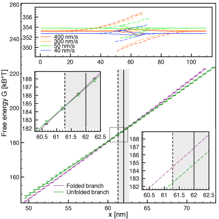
Figure 4: Free energy of the folded and unfolded branches. The purple line is $G_{N}(x)$, the dark green line is $G_{U}(x)$, both computed with respect to $G_{N}(x_{0})$. The black solid line and the gray area mark the expected value $x_{\mathrm{c}}=62.0(7)$ nm and its standard error, while the dashed black line is the crossing point $x_{\mathrm{c}}\approx 61.28$ nm. Both left and right insets show a magnified image of the coexistence region. In the right one, the dashed lines represent the free energies that we would obtain if we had overlooked the factor $\mathcal{P}^{U}_{N}$. The top panel shows the functions $\Delta G^{U}_{N}(x)-\Delta G^{U}_{U}(x)$ and $\Delta G^{N}_{N}(x)-\Delta G^{N}_{U}(x)$, which, by definition, should be independent of $x$ and equal to $G_{U}(x_{1})$. Again, the dashed lines represent the result if we do not include the factor $\mathcal{P}^{U}_{N}$.

In Fig. 3 (lower panel) we plot the function $z(u)$ for different pulling speeds. It is quite clear that the functions $z(u)$ are approximately constant along the $u$ axis and cross the line $z=u$ around the same value $G_{U}(\bar{x})=186.0(3)$. A distinctive aspect of Eq. (3) is the presence of the factor $\mathcal{P}^{U}_{N}$. If such correction was not taken into account then the fluctuation relation would not be satisfied anymore. We have verified that if ${P}^{U}_{N}$ is not included in the analysis, then the Bennett acceptance ratio method gives free energy estimates that depend on the pulling speed (see Supp. Mat.).

Free energy branches.

After having verified that the fluctuation relation Eq. (3) holds and that it can be used to extract the free energy of the unfolded ($G_{U}(\bar{x})$) and folded ($G_{N}(\bar{x})$, data not shown) branches, we have repeated the same procedure in a wide range of $x$ values. The range of values of $x$ is such that at least 8 trajectories go through $N$ (or $U$) (ensuring that we get a reasonable statistical significance). The results of the reconstruction of the free energy branches are shown in Fig. 4. The two free energy branches cross each other at a coexistence value $x_{c}$ at which the two states ($N$ and $U$) are equally probable. This is defined by $\Delta G_{N}^{U}(x_{c})=0$. We get $x_{\mathrm{c}}\approx 61.28$ nm, which is in good agreement with another estimate, $x_{\mathrm{c}}=62.0(7)$ nm, obtained interpreting experimental data according to a simple phenomenological model (see Supp. Mat.). In the insets of Fig. 4 we zoom the crossing region. It is interesting to recall again the importance of the aforementioned correction term ($\mathcal{P}^{U}_{N}$) to Eq. (3). If such term is not included in the analysis then the two reconstructed branches never cross (bottom right inset). This result is incompatible with the existence of the unfolding/refolding transition in the hairpin, showing that the factor $\mathcal{P}^{U}_{N}$ is key to measure free energy branches.

Equation (2) is valid in the very general situation of partially equilibrated initial states which, however, are arbitrarily far from global equilibrium. This makes the particular case Eq. (3) a very useful identity to recover the free energy of states that cannot be observed in conditions of thermodynamic global equilibrium. We have shown how it is possible to apply Eq. (3) to recover free energy differences of thermodynamic branches of folded and unfolded states in a two-state DNA hairpin. These methods can be further extended to the recovery of free energies of non-native states such as misfolded or intermediates states.