Inverse and Dynamical Supersymmetry Breaking in $S^{1}\times R^{3}$

Abstract

In this paper we study the influence of hard supersymmetry breaking terms in a $N=1$, $d=4$ supersymmetric model, in $S^{1}\times R^{3}$ spacetime topology. It is found that for some interaction terms and for certain values of the couplings, supersymmetry is unbroken for small lengths of the compact radius, and breaks dynamically as the radius increases. Also for another class of interaction terms, when the radius is large supersymmetry is unbroken and breaks dynamically as the radius decreases. It is pointed out that the two phenomena have similarities with the theory of metastable vacua at finite temperature and with the inverse symmetry breaking of continuous symmetries at finite temperature (where the role of the temperature is played by the compact dimension’s radius).

Introduction

Supersymmetry serves as the most promising extension of the Standard Model. In the short future supersymmetry will be verified experimentally through the LHC experiments. The elegance of the theory and the simplifications that introduces is of great importance however supersymmetry must be broken in our four dimensional world. There exist various mechanisms of supersymmetry breaking. In this article we are interested in dynamical breaking of supersymmetry induced from a toroidal compact dimension. Theories with one toroidal compact dimension resemble (mathematically) field theories at finite temperature. It is known that supersymmetry is spontaneously broken at finite temperature [26], a fact that is closely related to the boundary conditions that fermions and bosons obey in the ”thermal” compact dimension. Specifically supersymmetry is spontaneously broken due to the periodicity of bosonic degrees of freedom and anti-periodicity of the fermionic degrees of freedom. Field theories at finite temperature are conceptually related to field theories with compact dimensions. Thus it is easily understood that the boundary conditions of the fields in the compact dimensions control the breaking of supersymmetry. In general, when studying supersymmetric theories in flat spacetime, the background metric is ordinary Minkowski. Spacetime topology affect the boundary conditions of the fields that are integrated in the path integral. Given a class of metrics, several spacetime topologies are allowed. Here we shall focus on a model that has ${S}^{1}{\times R}^{3}$ topology underlying the spacetime, $S^{1}$ refers to a spatial dimension. The specific topology is a homogeneous topology of the flat Clifford–Klein type [16].  Non trivial topology, implies non trivial field configurations, that enter dynamically in the action. This non triviality enters in the action through the boundary conditions and as is well known the boundary conditions are controlled from the topology. The effective potential is a strong order parameter indicating when supersymmetry is broken. The appearance in the effective potential of vacuum terms which have different coefficients for fermions and bosons lead to the fact that the effective potential of the theory has no longer its minimum at zero and thus, supersymmetry is spontaneously broken. This quite general phenomenon can only be avoided in field theories with compact spatial dimensions, if in some way these vacuum terms are cancelled [30]. Indeed the combination of the allowed boundary conditions, as we show later, can save spontaneous supersymmetry breaking at finite volume. Particularly this is due to the fact that we can have periodic fermions and anti-periodic bosons. This cannot be avoided at finite temperature due to the restricted boundary conditions as we already mentioned, except in cases where fermions have a complex chemical potential [17] as in pure $SU(N)$ Yang Mills theories with adjoint fermions at finite temperature [18], namely,

$$\psi(\beta)=-e^{\frac{i2\pi k}{N}}\psi(0).$$ (1)

Normally a question arises while following the above considerations. Why should someone care in avoiding spontaneous supersymmetry breaking at finite volume? This is because when supersymmetry spontaneously breaks (like at finite temperature) then supersymmetry ceases to be a controllable symmetry of the theory, since it is always broken and not dynamically, but by definition. One would like to have control on the way that supersymmetry breaks (especially in our case that the model spacetime we work is 4 dimensional and supersymmetry must be a symmetry and be broken dynamically. This can be avoided in theories with higher dimensions where supersymmetry can hold in the higher dimensional space and break in our world).

In this paper we shall study a 4 dimensional N=1 supersymmetric model at one loop, in topology ${S}^{1}{\times R}^{3}$. We shall find the allowed field configurations that are determined from the topology and construct in a correct way the Lagrangian. The calculation of the effective potential follows, through which we shall find when supersymmetry breaks and when does not. After that we shall add in the Lagrangian non holomorphic and hard supersymmetry breaking terms. This terms break supersymmetry hardly. However for some values of the couplings and of the masses, interesting phenomena occur. Particularly it is found that in some cases when the volume of the compact space is small supersymmetry is not broken and when the compact radius exceeds a critical value, supersymmetry breaks dynamically. We shall give a cosmological implication of this case which resembles first order cosmological phase transitions in the early universe. Also other terms have a curious but worthy of mentioning effect. For these terms another strange phenomenon occurs for specific values of the couplings and masses. In detail for large values of the circumference of the compact dimension, supersymmetry is unbroken in contrast to the previous case and breaks after a critical length, as the compact dimension magnitude decreases. Although this is not so interesting from a phenomenological point of view (in four spacetime dimensions), it worths mentioning (and may have application in the physics of extra dimensions). There exist similar works in the literature but with the difference that the symmetry under study is not supersymmetry but a global symmetry (continuous or discrete). At finite temperature in some cases broken $O(N_{f})\times O(N_{\psi})$ symmetries become restored at high temperatures. Also unbroken symmetries at small temperatures may break at high temperatures (a phenomenon known as inverse symmetry breaking). The last may have cosmological implications. In our case the same occurs but with supersymmetry in place of the symmetry and for a compact dimension playing the temperature’s role (also note that roughly the high temperature limit is closely related to the small length limit through the transformation $T\rightarrow\frac{1}{L}$. Actually through the last transformation we can relate the two limits where this is possible). One interesting feature of this resemblance is the similarity of the terms in the lagrangian that trigger these phenomena in both cases. Also these terms appear in the new inflationary models and help in the procedure of reheating the universe after inflation. We shall present and describe everything in detail in the forthcoming sections. Also let us mention that our calculations will be in 1-loop level and within the perturbative limits with $mL\leq 1$, where $m$ is the largest mass scale in the theory and $L$ is the circumference of the compact dimension. Also within the four dimensional setup we use, renormalizability of masses and couplings is ensured when $mL\leq 1$.

In section 1 we review the mathematical setup needed for field theories with non trivial topology. The resemblance with extra dimensional theories is pointed out. In section 2 we describe the N=1 supersymmetric model we shall use and calculate the effective potential in the case of the compact dimension having infinite length and after that at finite volume. In section 3 we add several supersymmetry breaking terms and study in detail their effect on the vacuum energy of the model. In section 4 we review the continuous symmetry restoration, symmetry non-restoration and inverse symmetry breaking at finite temperature and point out the resemblance of these with our case (a resemblance that stems from the interactions of the scalar sector). In section 5 we present a cosmological application of one of our results and in section 6 a short discussion with the conclusions follow.

1 Non Trivial Topology, Twisted Fields and Supersymmetry

The existence of non trivial field configurations (in terms of boundary conditions) due to non trivial topology (twisted fields), was first pointed out by Isham [20] and then adopted by other authors [22, 21, 31]. In the spacetime of our case, the topological properties of $S^{1}{\times R}^{3}$ are classified by the first Stieffel class $H^{1}(S^{1}{\times R}^{3},Z_{\widetilde{2}})$ which is isomorphic to the singular (simplicial) cohomology group ${H}_{1}({S}^{1}{\times R}^{3}{,Z}_{2})$ because of the triviality of the ${Z}_{\widetilde{2}}$ sheaf. It is known that $H^{1}{(S}^{1}{\times R}^{3}{,Z}_{\widetilde{2}}{)=Z}_{2}$ classifies the twisting of a bundle. Specifically, it describes and classifies the orientability of a bundle globally. In our case, the classification group is ${Z}_{2}$ and, we have two locally equivalent bundles, which are however different globally i.e. cylinder-like and moebius strip-like. The mathematical lying behind, is to find the sections that correspond to these two bundles, classified completely by $Z_{2}$ [20]. The sections we shall consider are real scalar fields and Majorana spinor fields which carry a topological number called moebiosity (twist), which distinguishes between twisted and untwisted fields. The twisted fields obey anti-periodic boundary conditions, while untwisted fields periodic in the compactified dimension. Usually (inspired by field theory at finite temperature) one takes scalar fields to obey periodic and fermion fields anti-periodic boundary conditions, disregarding all other configurations that may arise from non trivial topology. We shall consider all these configurations. Let $\varphi_{u}$, $\varphi_{t}$ and $\psi_{t}$, $\psi_{u}$ denote the untwisted and twisted scalar and twisted and untwisted spinor fields respectively. The boundary conditions in the ${S}^{1}$ dimension are,

$$\varphi_{u}(x,0)=\varphi_{u}(x,L),$$ (2)

and

$$\varphi_{t}(x,0)=-\varphi_{t}(x,L),$$ (3)

for scalar fields and

$$\psi_{u}(x,0)=\psi_{u}(x,L),$$ (4)

and

$$\psi_{t}(x,0)=-\psi_{t}(x,L),$$ (5)

for fermion fields, where $x$ stands for the remaining two spatial and one time dimension which are not affected by the boundary conditions. Spinors (both Dirac and Majorana), still remain Grassmann quantities. We assign the untwisted fields twist ${h}_{0}$ (the trivial element of ${Z}_{2})$ and the twisted fields twist $h_{1}$ (the non trivial element of ${Z}_{2}$). Recall that $h_{0}+h_{0}=h_{0}$ ($0+0=0$), $h_{1}+h_{1}=h_{0}$ ($1+1=0$), $h_{1}+h_{0}=h_{1}$ ($1+0=1$). We require the Lagrangian to be scalar under $Z_{2}$ thus to have ${h}_{0}$ moebiosity. The topological charges flowing at the interaction vertices must sum to ${h}_{0}$ under ${H}^{1}{(S}^{1}{\times R}^{3}{,Z}_{\widetilde{2}}{)}$. For supersymmetric models, supersymmetry transformations impose some restrictions on the twist assignments of the superfield component fields [22].

Now which fields can acquire vacuum expectation value? Grassmann fields cannot acquire vacuum expectation value (vev) since we require the vacuum value to be a scalar representation of the Lorentz group. Thus, the question is focused on the two scalars. The twisted scalar cannot acquire non zero vev [21], consequently, only untwisted scalars are allowed to develop vev’s.

In the literature, twisted fields have frequently been used, for example in the Scherk-Schwarz mechanism [27], where the harmonic expansion of the fields is of the form:

$$\phi(x,y)=e^{imy}\sum_{n=-\infty}^{\infty}{\phi}_{n}(x)e^{\frac{i2{\pi}ny}{L}},$$ (6)

The ”$m$” parameter incorporates the twist mentioned above. This treatment is closely related to automorphic field theory [1] in more than 4 dimensions (which is an alternative to the one used by us). The Scherk-Schwarz mechanism is a well known mechanism that generates supersymmetry breaking to our 4 dimensional world after dimensional reduction and is frequently used for compactifications in extra dimensional models.

Concerning the automorphic field theory, let us quote here a different approach to the above. Due to the compact dimension we can use generic boundary conditions for bosons and fermions in the compact dimension. These are,

$$\varphi_{i}(x_{2},x_{3},\tau,x_{1}) = e^{i\pi n_{1}\alpha}\varphi_{i}(x_{2},x_{3},\tau,x_{1}+L)$$ (7)

$$~{}\Psi(x_{2},x_{3},\tau,x_{1}) = e^{i\pi n_{1}\delta}\Psi(x_{2},x_{3},\tau,x_{1}+L),$$

with, $0<\alpha,\delta<1$, $i=1,2$, $n_{1}=1,2,3...$. The values $\alpha=0,1$ correspond to periodic and antiperiodic bosons respectively while $\delta=0,1$ corresponds to periodic and anti-periodic fermions (for details see [1]).

2 Description of the Supersymmetric Model

The model we shall present is described by the global ${N=1}$, ${d=4}$ supersymmetric Lagrangian,

$$\mathcal{L}=[\Phi_{1}^{+}\Phi_{1}]_{D}+[\Phi^{+}\Phi]_{D}+[\frac{m_{1}}{2}\Phi^{2}+\frac{g_{1}}{6}\Phi^{3}+\frac{m}{2}\Phi_{1}^{2}+g\Phi\Phi_{1}^{2}]_{F}+{\rm{H.c}},$$ (8)

where $\Phi_{1}$, $\Phi$ are chiral superfields and the superpotential from which the interaction part of the lagrangian arises is $[\frac{m_{1}}{2}\Phi^{2}+\frac{g_{1}}{6}\Phi^{3}+\frac{m}{2}\Phi_{1}^{2}+g\Phi\Phi_{1}^{2}]_{F}$. In the above,

$$\Phi = \varphi_{u}(x)+\sqrt{2}\theta\psi_{u}(x)+\theta\theta F_{\varphi_{u}}+i\partial_{\mu}\varphi_{u}(x)\theta\sigma^{\mu}\bar{\theta}$$

$$-\frac{i}{\sqrt{2}}\theta\theta\partial_{\mu}\psi_{u}(x)\sigma^{\mu}\bar{\theta}-\frac{1}{4}\partial_{\mu}\partial^{\mu}\varphi_{u}^{+}(x)\theta\theta\bar{\theta}\bar{\theta},$$

is a left chiral superfield. It contains the untwisted scalar field components and the untwisted Weyl fermion. Although the untwisted scalar is complex, we shall use the real components which will be the representatives of the sections of the trivial bundle classified by ${H}^{1}{(S}^{1}{\times R}^{3}{,Z}_{\widetilde{2}}{)}$. Moreover,

$$\Phi_{1} = \varphi_{t}(x)+\sqrt{2}\theta\psi_{t}(x)+\theta\theta F_{\varphi_{t}}+i\partial_{\mu}\varphi_{t}(x)\theta\sigma^{\mu}\bar{\theta}$$

$$-\frac{i}{\sqrt{2}}\theta\theta\partial_{\mu}\psi_{t}(x)\sigma^{\mu}\bar{\theta}-\frac{1}{4}\partial_{\mu}\partial^{\mu}\varphi_{t}^{+}(x)\theta\theta\bar{\theta}\bar{\theta},$$

is another left chiral superfield containing the twisted scalar field and the twisted Weyl fermion. Writing down (8) in component form, we get (writing Weyl fermions in the Majorana representation):

$$\mathcal{L} =\partial_{\mu}\varphi_{u}^{+}\partial^{\mu}\varphi_{u}-\left|m_{1}\varphi_{u}+\frac{g_{1}}{2}\varphi_{u}\varphi_{u}+g\varphi_{t}^{2}\right|^{2}+i\overline{\Psi}_{t}\gamma^{\mu}\partial_{\mu}\Psi_{t}-\frac{1}{2}m\overline{\Psi}_{t}\Psi_{t}$$ (11)

$$-\frac{g_{1}}{4}(\overline{\Psi}_{u}\Psi_{u}-\overline{\Psi}_{u}\gamma_{5}\Psi_{u})\varphi_{u}-\frac{g_{1}}{4}(\overline{\Psi}_{u}\Psi_{u}+\overline{\Psi}_{u}\gamma_{5}\Psi_{u})\varphi_{u}^{+}+\partial_{\mu}\varphi_{t}^{+}\partial^{\mu}\varphi_{t}-$$

$$\left|m\varphi_{t}+2g\varphi_{t}\varphi_{u}\right|^{2}+i\overline{\Psi}_{u}\gamma^{\mu}\partial_{\mu}\Psi_{u}-\frac{1}{2}m_{1}\overline{\Psi}_{u}\Psi_{u}-$$

$$\frac{g}{4}(\overline{\Psi}_{t}\Psi_{t}-\overline{\Psi}_{t}\gamma_{5}\Psi_{t})\varphi_{u}-\frac{g}{4}(\overline{\Psi}_{t}\Psi_{t}+\overline{\Psi}_{t}\gamma_{5}\Psi_{t})\varphi_{u}^{+}.$$

Notice that moebiosity is conserved at all interaction vertices i.e. equals ${h}_{0}$. The moebiosity of $\varphi_{u}$ and $\Psi_{u}$ is ${h}_{0}$ while for $\varphi_{t}$ and $\Psi_{t}$ is ${h}_{1}$. Using the ${Z}_{2}$ cyclic group properties we see that the Lagrangian (11) has moebiosity ${h}_{0}$. The complex field $\varphi_{u}$ can be written in terms of real components as ${\varphi}_{u}{=\chi+i\varphi}_{u_{2}}{/}\sqrt{2}$, where $\chi={v+(\varphi}_{u_{1}}{)/}\sqrt{2}$ (${v}$ is the classical value). Thus, $\varphi_{u_{1}}$ and $\varphi_{u_{2}}$ are real untwisted field configurations belonging to the trivial element of ${H}^{1}{(S}^{1}{\times R}^{3}{,{Z}_{\widetilde{2}})}$ and satisfying periodic boundary conditions in the compactified dimension. The twisted scalar field can be written as ${\varphi}_{t}{=(\varphi}_{t_{1}}{+i\varphi}_{t_{2}}{)/}\sqrt{2}$, since, this field, being a member of the non trivial element of ${H}^{1}{(S}^{1}{\times R}^{3}{,Z}_{\widetilde{2}}{)}$ cannot acquire a vev. Notice we gave a vev for an untwisted boson, This is useful in order to find the minimum of the effective potential minimizing it in terms of $v$. The masses of the two Majorana fermion fields and the four bosonic fields at tree order are calculated to be:

$$m_{b_{1}}^{2} = m_{1}^{2}+3g_{1}m_{1}v+3g_{1}^{2}v^{2}/2$$ (12)

$$\ m_{b_{2}}^{2} = m_{1}^{2}+g_{1}m_{1}v+g_{1}^{2}v^{2}/2$$

$$m_{t_{1}}^{2}\vskip 12.0pt plus 4.0pt minus 4.0pt = m^{2}+4gmv+4g^{2}v^{2}+g^{2}m_{1}v/\sqrt{2}+g^{2}g_{1}v^{2}/4\$$

$$\ m_{t_{2}}^{2} = m^{2}+4gmv-g^{2}m_{1}v/\sqrt{2}-g^{2}g_{1}v^{2}/4$$

$$m_{f_{1}} = m_{1}+g_{1}v,\ m_{f_{2}}=m+2gv.$$

In (12) $m_{b_{1}}$, $m_{b_{2}}$ are the masses of the untwisted bosons (${\varphi}_{u_{1}}$ and ${\varphi}_{u_{2}}$ respectively), $m_{t_{1}}$, $m_{t_{2}}$ are the masses of the twisted bosons (${\varphi}_{t_{1}}$ and ${\varphi}_{t_{2}}$) and, finally, $m_{f_{1}}$, $m_{f_{2}}$ are the untwisted Majorana fermion and twisted Majorana fermion masses respectively ($\Psi_{u}$ and $\Psi_{t}$). The general tree level result for theories with rigid supersymmetry in terms of chiral superfields is satisfied (see [24]) i.e. :

$$STr(M^{2})=\sum\limits_{j}(-1)^{2j}(2j+1)m_{j}^{2}=0.$$ (13)

Also, the following relations hold true:

$$m_{b_{1}}^{2}+m_{b_{2}}^{2}=2m_{f_{1}}^{2},\ m_{t_{1}}^{2}+m_{t_{2}}^{2}=2m_{f_{2}}^{2}.$$ (14)

Since twisted scalars cannot acquire vacuum expectation value, supersymmetry is not spontaneously broken at tree level, like in the O’ Raifeartaigh models. Indeed the auxiliary field equations,

$$F_{\varphi_{u}}^{+} = m_{1}\varphi_{u}+\frac{g_{1}}{2}\varphi_{u}^{2}+g\varphi_{t}^{2}=0$$ (15)

$$F_{\varphi_{t}}^{+} = m\varphi_{t}+2g\varphi_{u}\varphi_{t}=0,$$

imply that $\varphi_{u}=0$ and $\varphi_{t}=0$ and consequently $v=0$, thus, at tree level, no spontaneous supersymmetry breaking occurs.

2.1 Supersymmetric Effective Potential in $S^{1}\times R^{3}$

We now proceed by assuming that the topology is changed to ${S}^{1}{\times R}^{3}$, while the local geometry remains Minkowski. The metric reads:

$$\mathrm{d}s^{2}=\mathrm{d}t^{2}-\mathrm{d}x_{1}^{2}-\mathrm{d}x_{2}^{2}-\mathrm{d}x_{3}^{2},$$ (16)

with $-\infty<x_{2},x_{3},t<\infty$ and $0<x_{1}<L$ with the points${\ x}_{1}=0~{}$and ${x}_{1}=L$ periodically identified. The boundary conditions for the fields are:

$$~{}\varphi_{u}(x_{1},x_{2},x_{3},t) =~{}~{}~{}~{}~{}\varphi_{u}(x_{1}+L,x_{2},x_{3},t)$$ (17)

$$~{}\varphi_{t}(x_{1},x_{2},x_{3},t) =~{}{}-\varphi_{t}(x_{1}+L,x_{2},x_{3},t)$$

$$~{}\Psi_{u}(x_{1},x_{2},x_{3},t) =~{}~{}~{}~{}~{}\Psi_{u}(x_{1}+L,x_{2},x_{3},t)$$

$$~{}\Psi_{t}(x_{1},x_{2},x_{3},t) =~{}~{}-\Psi_{t}(x_{1}+L,x_{2},x_{3},t).$$

We Wick rotate the time direction ${t}\rightarrow{it}$ thus giving the background metric the Euclidean signature [31]. The twisted fermions and twisted bosons will be summed over odd Matsubara frequencies, while the untwisted fermions and untwisted scalars will be summed over even Matsubara frequencies [19, 23]. Adopting the $\overline{DR}^{\prime}$ renormalization scheme [24] the Euclidean effective potential at one loop level reads:

$$V =V_{0}+\frac{1}{64\pi^{2}L}\sum\limits_{n=-\infty}^{\infty}\int\frac{\mathrm{d}^{3}k}{(2\pi)^{3}}{\bigg{(}}\ln[k^{2}+\frac{4\pi^{2}n^{2}}{L^{2}}+m_{b_{1}}^{2}]$$ (18)

$$-2\ln[k^{2}+\frac{4\pi^{2}n^{2}}{L^{2}}+m_{f_{1}}^{2}]+\ln[k^{2}+\frac{4\pi^{2}n^{2}}{L^{2}}+m_{b_{2}}^{2}]$$

$$-2\ln[k^{2}+\frac{\pi^{2}(2n+1)^{2}}{L^{2}}+m_{f_{2}}^{2}]+\ln[k^{2}+\frac{\pi^{2}(2n+1)^{2}}{L^{2}}+m_{t_{1}}^{2}]$$

$$+\ln[k^{2}+\frac{\pi^{2}(2n+1)^{2}}{L^{2}}+m_{t_{2}}^{2}]{\bigg{)}.}$$

${V}_{0}~{}$includes the tree and the one loop corrections for infinite length,

$$V_{0} =m_{1}^{2}v^{2}+g_{1}^{2}m_{1}v^{3}+\frac{g_{1}^{2}v^{4}}{4}+\frac{1}{64\pi^{2}}{\bigg{(}}m_{b_{1}}^{4}(\ln[\frac{m_{b_{1}}^{2}}{\mu^{2}}]-\frac{3}{2})$$ (19)

$$+m_{b_{2}}^{4}(\ln[\frac{m_{b_{2}}^{2}}{\mu^{2}}]-\frac{3}{2})+m_{t_{1}}^{4}(\ln[\frac{m_{t_{1}}^{2}}{\mu^{2}}]-\frac{3}{2})+m_{t_{2}}^{4}(\ln[\frac{m_{t_{2}}^{2}}{\mu^{2}}]-\frac{3}{2})$$

$$-2m_{f_{1}}^{4}(\ln[\frac{m_{f_{1}}^{2}}{\mu^{2}}]-\frac{3}{2})-2m_{f_{2}}^{4}(\ln[\frac{m_{f_{2}}^{2}}{\mu^{2}}]-\frac{3}{2}){\bigg{)}},$$

and $\mu$ is the renormalization scale, being of the order of the largest mass [28]. Furthermore, we shall assume that $m{L\simeq 1}$ which is required for the validity of perturbation theory [36, 29].

2.2 How Can Supersymmetry be Broken Spontaneously in $S^{1}\times R^{3}$

It is well known that when one considers only twisted fermions and untwisted bosons in ${S}^{1}{\times R}^{3}$ (like in thermal field theories), vacuum contributions $\sim$${L}^{-4}$ do not cancel and supersymmetry is spontaneously broken. The non-cancellation occurs because bosons and fermions satisfy different boundary conditions. In our model the field content is such that cancellation of vacuum contributions is being enforced, after having included all topologically inequivalent allowed field configurations. This situation is similar to finite temperature calculations. The question if supersymmetry is broken or not requires to check the zero modes of the vacuum state [25]. It is easy to see why in conventional finite temperature field theories and their conceptional analogues ${S}^{1}{\times R}^{3}$ topological field theories supersymmetry is broken. The vacuum state, in the Wess–Zumino in ${S}^{1}{\times R}^{3}$, does contain one bosonic zero mode. In our case this does not occur because we have equal vacuum zero modes (twisted spinors, do not have a zero mode). Consequently, in our model, we expect that supersymmetry will not be spontaneously broken [30] (for a detailed discussion we recommend the paper of Fujikawa [26]).

2.3 Small $L$ Expansion of the effective potential

The leading order contribution to the one loop effective potential for small $L$ values is given by [19, 33, 7]:

$$V=m_{1}^{2}v^{2}+g_{1}^{2}m_{1}v^{3}+\frac{g_{1}^{2}v^{4}}{4}$$ (20)

$${-\frac{3(2m_{f_{1}}^{4}-m_{b_{1}}^{4}-m_{b_{2}}^{4})}{4096\pi^{4}}-\frac{3(2m_{f_{2}}^{4}-m_{t_{1}}^{4}-m_{t_{2}}^{4})}{256\pi^{4}}}$$

$${+\frac{3(2m_{f_{1}}^{4}-m_{b_{1}}^{4}-m_{b_{2}}^{4}+2m_{f_{2}}^{4}-m_{t_{1}}^{4}-m_{t_{2}}^{4})}{128\pi^{2}}}$$

$${+\frac{(\gamma-\ln[4\pi])(2m_{f_{1}}^{4}-m_{b_{1}}^{4}-m_{b_{2}}^{4})}{1024\pi^{4}}+\frac{(\gamma+\ln[\frac{2}{\pi}])(2m_{f_{2}}^{4}-m_{t_{1}}^{4}-m_{t_{2}}^{4})}{64\pi^{4}}}$$

$${+\frac{(2m_{f_{1}}^{3}-m_{b_{1}}^{3}-m_{b_{2}}^{3})}{384L\pi^{3}}-\frac{(2m_{f_{1}}^{2}-m_{b_{1}}^{2}-m_{b_{2}}^{2})}{768\pi^{2}L^{2}}+\frac{(2m_{f_{2}}^{2}-m_{t_{1}}^{2}-m_{t_{2}}^{2})}{384\pi^{2}L^{2}}}$$

$${+\frac{2m_{f_{1}}^{4}\ln[Lm_{f_{1}}]-m_{b_{2}}^{4}\ln[Lm_{b_{2}}]-m_{b_{1}}^{4}\ln[Lm_{b_{1}}]}{1024\pi^{4}}}$$

$${+\frac{2m_{f_{2}}^{4}\ln[Lm_{f_{2}}]-m_{t_{2}}^{4}\ln[Lm_{t_{2}}]-m_{t_{1}}^{4}\ln[Lm_{t_{1}}]}{64\pi^{4}}}$$

$${-\frac{(2m_{f_{1}}^{4}\ln[\frac{m_{f_{1}}^{2}}{\mu^{2}}]-m_{b_{2}}^{4}\ln[\frac{m_{b_{2}}^{2}}{\mu^{2}}]-m_{b_{1}}^{4}\ln[\frac{m_{b_{1}}^{2}}{\mu^{2}}])}{64\pi^{2}}}$$

$${-\frac{(2m_{f_{2}}^{4}\ln[\frac{m_{f_{2}}^{2}}{\mu^{2}}]-m_{t_{2}}^{4}\ln[\frac{m_{t_{2}}^{2}}{\mu^{2}}]-m_{t_{1}}^{4}\ln[\frac{m_{t_{1}}^{2}}{\mu^{2}}])}{64\pi^{2}}.}$$

Figure 1: The supersymmetric effective potential

Since relation (14) holds, the terms proportional to $\frac{1}{L^{2}}$ cancel [30]. Also, the minimum of the potential vanishes at ${v=}$0 and supersymmetry is preserved. Indeed, expanding (20) for small ${v}$ we get:

$$V\simeq m_{1}^{2}v^{2}+O(v^{3}).$$ (21)

In figure 1 we plot the effective potential for the upper perturbative limit $mL=1$. The other numerical values are chosen to be: ${m}_{1}{=}$200, ${m=}$7000, ${g}_{1}{=}$0.001, ${g=}$0.09, ${\mu=}$7000.

3 Addition of Explicit Supersymmetry Breaking Terms

Let us now introduce into the Lagrangian (11) various hard supersymmetry breaking terms of the form $g_{3}\chi^{2}\varphi_{i}^{2}$ and $g_{2}\overline{\psi}\psi\chi$, where ${g}_{3}$ and $g_{2}$ are dimensionless couplings (and recall $\chi=v+\varphi_{u_{1}}/\sqrt{2}$). This terms, being non holomorphic and hard, break supersymmetry explicitly (also these terms have moebiosity zero).

Indeed the addition of such terms re-introduces quadratic divergences in the theory, namely,

$$\Delta m_{scalar}=\frac{1}{8\pi^{2}}(l_{s}-l_{f}^{2})\Lambda^{2}_{UV},$$ (22)

with $\Lambda^{2}_{UV}$ a relevant upper cut-off of the theory and $l_{s}$, $l_{f}$ boson and fermion couplings.

Since $\chi$ develops a vev, the fields coupled to it will acquire an additional mass of the form $g_{3}v^{2}$ and $g_{2}v$. We can add various combinations of the allowed terms. There exist two class of phenomena occurring, depending on the supersymmetry breaking terms we use.

The first type and, from a phenomenological point of view more interesting, resembles the first order phase transition picture in thermal field theory. Actually, regardless that there exist hard supersymmetry breaking terms, supersymmetry is unbroken for small values of the length of the compact dimension $L$. The minimum of the potential is zero at $v=0$, $V(0)=0$. As the length of the compact dimension increases, a second non supersymmetric minimum is created after a critical length is reached. Then phenomena may occur that can be described by the theory of metastable vacua (the reader may find useful the papers [6, 7] where similar issues are discussed in $S^{1}\times R^{3}$ but for a non supersymmetric $\phi^{4}$ theory. Again non trivial topology induces similar behavior of the effective potential).

The second type of phenomena describes a theory that supersymmetry is unbroken when the length of the compact dimension is large and as the radius decreases, supersymmetry breaks spontaneously after a critical length. Thus supersymmetry is broken only for small lengths. Although this is rather curious for a four dimensional model, we shall present it because it may have application to extra dimensional models.

3.1 A term of the form $g_{3}\chi^{2}\varphi_{u_{2}}^{2}$

We introduce into the Lagrangian (11) an interaction term between the two untwisted scalar fields, of the form $-g_{3}\chi^{2}\varphi_{u_{2}}^{2}$. Since $\chi=v+\varphi_{u_{1}}/\sqrt{2}$, the scalar field $\varphi_{u_{2}}$ will acquire an additional mass term of the form $g_{3}v^{2}$. This way, the masses of the fields now become:

$$m_{b_{1}}^{2} = m_{1}^{2}+3g_{1}m_{1}v+3g_{1}^{2}v^{2}/2$$ (23)

$$\ m_{b_{2}}^{2} = m_{1}^{2}+g_{1}m_{1}v+g_{1}^{2}v^{2}/2+g_{3}v^{2}$$

$$m_{t_{1}}^{2}\vskip 12.0pt plus 4.0pt minus 4.0pt = m^{2}+4gmv+4g^{2}v^{2}+g^{2}m_{1}v/\sqrt{2}+g^{2}g_{1}v^{2}/4$$

$$\ m_{t_{2}}^{2} = m^{2}+4gmv-g^{2}m_{1}v/\sqrt{2}-g^{2}g_{1}v^{2}/4$$

$$m_{f_{1}} = m_{1}+g_{1}v,\ m_{f_{2}}=m+2gv.$$

As expected, supersymmetry is now broken and relation (13) becomes,

$$2m_{f_{1}}^{2}-m_{b_{1}}^{2}-m_{b_{2}}^{2}=g_{3}v^{2},\ m_{t_{1}}^{2}+m_{t_{2}}^{2}=2m_{f_{2}}^{2}.$$ (24)

One can see that the supersymmetric minimum at $v=0$ is still preserved. Indeed, $V$ can be written as:

$$V\simeq(m_{1}^{2}+\frac{g_{3}}{768\pi^{2}L^{2}})v^{2}+O(v^{3}).$$ (25)

We can see that in the continuum limit (infinite $L$), the supersymmetric vacuum becomes metastable and a second non supersymmetric vacuum appears. Including finite size corrections, we see that for small ${L}$ the effective potential has a unique supersymmetric minimum at $v=0$. As ${L}$ increases, a second minimum develops, which becomes supersymmetric at the critical value ${L}_{c}{=}\frac{1}{21571}$. When ${L}\!>\!{L}_{c}$ the second minimum is non supersymmetric and becomes energetically more preferable than the supersymmetric one [32, 34]. This said behavior of the potential is valid whenever $g_{3}\gg g_{1}$ and for $\frac{m_{1}}{m}\ll g_{3}$. Using the same numerical values as before, we plot the effective potential for ${g}_{3}{=}$0.5, first in the continuum limit (figure 2), and then including ${L}$ dependent corrections (figure 3).

Figure 2: The continuum effective potential

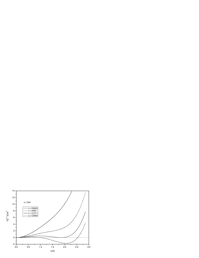
Figure 3: The effective potential including finite size corrections

Let us discuss the above results. $g_{3}$, $g_{1}$ are couplings among the untwisted superfields, $g_{3}$ corresponding to the supersymmetry breaking term. If the $g_{3}$ interaction is stronger than $g_{1}$ and if the mass (${m}$) of the twisted superfield is larger than the untwisted one (${m_{1}}$), then the following phenomenon occurs. For small length ${L}$ of the compact dimension, supersymmetry is not broken (figure 3). As ${L}$ grows larger, a second minimum appears which is not supersymmetric (${L}\!>\!{L}_{c}$). There exists a small barrier separating the two minima (figure 3), and there exists the possibility of quantum barrier penetration between them. This resembles the first order phase transition picture of thermal field theories.

Upon closer examination, we can see that in the continuum limit, the supersymmetric vacuum becomes metastable and a second non supersymmetric vacuum appears. Including finite size corrections, we see that for small ${L}$ the effective potential has a unique supersymmetric minimum at $v=$0. As ${L}$ increases, a second minimum develops, which becomes supersymmetric at the critical value ${L}_{c}{=}\frac{1}{21571}$. When ${L}\!>\!{L}_{c}$ the second minimum breaks supersymmetry and becomes energetically more preferable than the supersymmetric one [32, 34]. This said behavior of the potential is always valid whenever $g_{3}\gg g_{1}$ and for $\frac{m_{1}}{m}\ll g_{3}$. Using the same numerical values as before, we plot the effective potential for ${g}_{3}{=}$0.5, first in the continuum limit (figure 2), and then including ${L}$ dependent corrections (figure 3).

3.2 A term of the form $g_{3}\chi^{2}\varphi_{t_{1}}^{2}$

Let us try something different now. We add an interaction among a twisted boson and the untwisted boson that acquires vev, namely $-g_{3}\chi^{2}\varphi_{t_{1}}^{2}$. Since $\chi=v+\varphi_{u_{1}}/\sqrt{2}$ the twisted boson $\varphi_{t_{1}}$ will have additional contribution to it’s tree order mass. The masses now read,

$$m_{b_{1}}^{2} = m_{1}^{2}+3g_{1}m_{1}v+3g_{1}^{2}v^{2}/2$$ (26)

$$\ m_{b_{2}}^{2} = m_{1}^{2}+g_{1}m_{1}v+g_{1}^{2}v^{2}/2$$

$$m_{t_{1}}^{2}\vskip 12.0pt plus 4.0pt minus 4.0pt = m^{2}+4gmv+4g^{2}v^{2}+g^{2}m_{1}v/\sqrt{2}+g^{2}g_{1}v^{2}/4+g_{3}v^{2}$$

$$\ m_{t_{2}}^{2} = m^{2}+4gmv-g^{2}m_{1}v/\sqrt{2}-g^{2}g_{1}v^{2}/4$$

$$m_{f_{1}} = m_{1}+g_{1}v,\ m_{f_{2}}=m+2gv.$$

As expected $m_{t_{1}}^{2}+m_{t_{2}}^{2}-2m_{f_{2}}^{2}\neq 0$, since supersymmetry is hard broken.

An interesting phenomenon occurs for this term and for a class of other terms as we shall see. In detail, when the length of the compact dimension is small, supersymmetry is broken and becomes restored when the radius increases (and overcomes a critical length $L_{c}$).

This is strange and rather counterintuitive to what would be expected from a phenomenologically correct four dimensional theory. However we describe it since it might be useful to extra dimensional physics. Also, as we shall see in the next section, the whole behavior resembles the inverse symmetry breaking of continuous symmetries at finite temperature. Let us call it ”inverse supersymmetry breaking” for brevity. This said behavior can appear when $g_{3}$ is of the order of $\frac{m_{1}}{m}$ or for values smaller, that is $g_{3}\leq\frac{m_{1}}{m}$ when only the term $g_{3}\chi^{2}\varphi_{t_{1}}^{2}$ appears in the Lagrangian (recall that in the previous subsection, the metastable vacua phenomena of the previous subsection occurred when $\frac{m_{1}}{m}\ll g_{3}$). This whole phenomenon is well seen in figure 4. We used the following numerical values, ${m}_{1}{=}$200, ${m=}$7000, ${g}_{1}{=}$0.001, ${g=}$0.09, ${\mu=}$7000 and $g_{3}=0.05$.

Figure 4: Inverse Supersymmetry Breaking

As can be seen in figure 4 the phenomenon looks like a second order phase transition with the length of the compact dimension playing the role of the temperature. No barrier appears between the vacua at $v=0$ and at $v\neq 0$. The study was limited to perturbation preserving values of $L$. As we see for large $L$ ($L=1/7000$) supersymmetry is unbroken and start’s to break at $L_{c}=1/50830$. As the length decreases, the breaking is more profound. The two non supersymmetric vacua are not equivalent.

$g_{3}$	$L_{c}^{-1}$
0.1	32319
0.07	41352
0.05	50839
0.03	67994
0.01	121950
0.007	145900
0.005	173083
0.003	223990
0.001	388990
0.0005	557000
0.0001	1232000
0.00005	1740000
0.00001	3942000

Values of $g_{3}$ and corresponding $L_{c}$

We tried to find how $L_{c}$ changes under a change of $g_{3}$. In the table we present the values of $g_{3}$ and the corresponding values of $L_{c}$, and in figure 5 we plot the dependence. In figure 6 we fit the curve with a continuous function. The dots are the values that appear in the table, while the continuous line corresponds to the function $0.000091\sqrt{x}$. Thus the dependence of $g_{3}$ as a function of $L_{c}$ is roughly,

$$g_{3}\sim 0.000091\sqrt{L_{c}}.$$ (27)

Figure 5: Plot of $g_{3}$ and $L_{c}$

Figure 6: Fit of the curve $g_{3}-L_{c}$

3.3 Other Hard Supersymmetry Breaking terms and Discussion

We shall not present here the detailed study of all the allowed terms (this will be done in [15]). We shall discuss only the main results.

A term of the form $g_{2}\overline{\psi_{i}}\psi_{i}\chi$ always breaks supersymmetry and non of the previous phenomena occurs. As we shall see in the next section this is similar to symmetry non restoration where a continuous symmetry is broken and never get’s restored.

The combined addition of terms $-\frac{1}{2}g_{2}\overline{\psi_{t}}\psi_{t}\chi-g_{3}\chi^{2}\varphi_{t_{1}}^{2}$ (that is interaction of the untwisted scalar $\chi$ with a twisted fermion and twisted boson) causes ”inverse supersymmetry breaking” as previous. The conditions that must hold in order this occurs are the same as before ($g_{3}\leq\frac{m_{1}}{m}$) and in addition $g_{2}\ll g_{3}$. For this condition the behavior of supersymmetry breaking is well described from figure 4. Also for $g_{2}=0.0001$ the $g_{3}-L_{c}$ dependence is similar to that of figure 6. Particularly the $g_{3}-L_{c}$ dependence in this case, is described by,

$$g_{3}\sim 0.000091\sqrt{L_{c}},$$ (28)

which is the same as before. This dependence is the same for all the cases we studied. Thus this motivates us to think that there is a universal behavior of $g_{3}$ as a function of $L_{c}$.

Of course all effects we described in this section appear in one loop level and within perturbative limits. Thus there exist the danger that all these effects are an artifact of perturbation theory. However the theory is at some level supersymmetric and one loop corrections may be adequate enough [24]. A detailed study should include higher loop corrections. In the next section similar problems-considerations are encountered and discussed.

4 Continuous and Discrete Symmetry Inverse Symmetry Breaking, Restoration and Non-restoration at Finite Temperature

In this section we review some conceptually similar phenomena to the above. The difference is that symmetries are studied at finite temperature and the symmetry is not supersymmetry but a continuous global $O(N_{1})\times O(N_{2})$ or a discrete $Z_{2}\times Z_{2}$. As we shall see symmetry non-restoration and inverse symmetry breaking phenomena occur naturally when similar terms to $\frac{1}{2}g_{2}\overline{\psi_{t}}\psi_{t}\chi$, $g_{3}\chi^{2}\varphi_{t_{1}}^{2}$ appear in the Lagrangian.

Symmetry non-restoration means that a symmetry broken at $T=0$ never gets restored at high temperatures. Inverse symmetry breaking means that an unbroken symmetry at $T=0$ may be spontaneously broken at high temperature.

These phenomena occur in field theories when cross interactions are included among the scalar fields similar to the bosonic hard supersymmetry breaking term $g_{3}\chi^{2}\varphi_{u_{2}}^{2}$. Similar to this term scalar interactions and also Yukawa terms like the ones of the previous sections are frequently used in the theory of reheating after inflation. Actually this similarities motivated us to use such terms in order to see what their effect would be on supersymmetry breaking. We shall discuss these in the end of this section.

First let us describe the inverse symmetry breaking phenomenon. Consider a theory with real scalar fields $\phi_{1}$ and $\phi_{2}$ described by the $O(N_{1})\times O(N_{2})$ globally symmetric Lagrangian,

$$L=\frac{1}{2}\partial_{\mu}\phi_{1}\partial_{\mu}\phi_{1}+\frac{1}{2}\partial_{\mu}\phi_{2}\partial_{\mu}\phi_{2}+\frac{1}{2}m_{1}^{2}\phi_{1}^{2}+\frac{1}{2}m_{2}^{2}\phi_{2}^{2}+\frac{1}{4!}\lambda_{1}\phi_{1}^{4}+\frac{1}{4!}\lambda_{1}\phi_{2}^{4}+\frac{1}{4!}\lambda\phi_{1}^{2}\phi_{2}^{4},$$ (29)

where $\phi_{1}$ and $\phi_{2}$ be real scalars with $N_{1}$ and $N_{2}$ components. In the above Lagrangian one of the global $O(N_{i})$ symmetries may break at high temperature if the $\lambda$ coupling takes negative values. Thus one of the two scalar fields $\phi_{1}$ or $\phi_{2}$ may acquire a non zero vacuum expectation value. Thus at high temperature and for certain values of the parameters, the initial $O(N_{1})\times O(N_{2})$ is broken to $O(N_{1})$. This was called inverse symmetry breaking and was first point out by Weinberg [14] and extensively studied by many authors [2, 3, 4, 5, 8, 9, 10].

In the case $N_{1}=1$ and $N_{2}=1$ the initial $O(N_{1})\times O(N_{2})$ symmetry reduces to a $Z_{2}\times Z_{2}$ symmetry and similar arguments hold, in connection to the breaking of one of the two discrete symmetries (for details see [4])

Symmetry non-restoration was used in [8] to solve the monopole problem in the $SU(5)$ GUT. Monopoles are usually produced during phase transitions at temperatures of the order $\sim 10^{14}$GeV. As was proposed in [8], the symmetric phase of $SU(5)$ was never realized, no matter how high the temperature becomes. In that paper the interaction term $\alpha|\chi_{45}|^{2}|H_{24}|$ appearing in the scalar Kibble-Higgs sector is responsible for the non-restoration of the $SU(5)$ symmetry. Actually the scalar interaction of $H_{24}$ and $\chi_{45}$ gives negative contributions to the thermal masses and one of those becomes negative. Once this happens the corresponding Higgs field maintains a vacuum expectation value for high temperatures and the symmetry is never restored. This phenomenon occurs for certain values of the parameters (see [8, 3]). However these results are very sensitive and are altered when someone includes two loop calculations [3]. In the same spirit there are arguments based on large N calculations which can show that symmetry non-restoration is an artifact of perturbation theory. For an interesting discussion on this see [3] and references therein.

A cross term of the form $g\chi^{2}\phi^{2}$ is used in non relativistic models in condensed matter physics, for example in the coupled two field Bose gases. However the effect of this does not break any of the initial symmetry patterns [9].

In conclusion the intuitive approach to all phenomena at finite temperature consists of the statement that symmetries broken at small temperatures become restored at high temperature (in the same class belong finite volume theories). Many field theory models exist that belong to this class. Counter intuitive phenomena occur in field theories with rich scalar sector. Especially if the multi-scalar sectors interact weakly with negative couplings then the phenomena known as inverse symmetry breaking or symmetry non-restoration occur. This happens at high temperature and refers to the spontaneous breaking of a symmetry at high temperature. Usually the symmetry is a global $O(N_{1})\times O(N_{2})$ or for the case of symmetry non-restoration a continuous, like $SU(5)$.

Although inverse symmetry breaking is counterintuitive, nature has provided us with examples that systems are more symmetric at low temperatures than at high temperature. For example the Rochelle salt which at low temperatures is orthorhombic and after a critical temperature becomes monoclinic. Similar phenomena occur in liquid crystals (for more examples see [10] and references therein).

4.1 Reheating After Inflation and Thermal Inflation

The process of reheating after inflation is one of the most important features of the new inflationary scenario [11]. The process of reheating is necessary in order that the inflating vacuum like state of the universe transforms to a hot Friedmann universe state. During the reheating process a massive scalar field gives it’s vacuum energy to lighter fermions and bosons. The Lagrangian governing this process is,

$$L=\frac{1}{2}(\partial_{\mu}\varphi)^{2}-\frac{m_{\varphi}}{2}\varphi^{2}+\frac{1}{2}(\partial_{\mu}\chi)^{2}-\frac{m_{\chi}}{2}\chi^{2}+\overline{\psi}(i\gamma^{\mu}\partial_{\mu}-m_{\psi})\psi-\lambda\varphi\overline{\psi}\psi-\frac{1}{2}g^{2}\varphi^{2}\chi^{2}.$$ (30)

The role of the inflaton fields is played from the scalar field $\varphi$. The inflaton field decays to the particles $\psi$ and $\chi$ due to the interaction terms $\lambda\varphi\overline{\psi}\psi$ and $\frac{1}{2}g^{2}\varphi^{2}\chi^{2}$. Note that we used similar terms in order to break supersymmetry hard and all the effects we seen in the previous section are due to these interaction terms. Also, in order reheating takes place, the condition $m_{\varphi}\gg m_{\psi},m_{\varphi}$ must hold (remember that similar conditions hold in the supersymmetric model we studied previously. There $m_{1}$ was the tree order mass of the untwisted scalar field and $m$ the tree order mass of the twisted scalar. One of the conditions we used is that the untwisted sector has greater mass than the twisted sector, namely $m_{1}\gg m$. Also the untwisted fermion has mass m).

So with the interactions $\lambda\varphi\overline{\psi}\psi$ and $\frac{1}{2}g^{2}\varphi^{2}\chi^{2}$ the initially concentrated energy (during inflation) to the field $\varphi$ is transferred to particle creation through the processes $\varphi\rightarrow\psi\psi$ and $\varphi\rightarrow\chi\chi$, and the universe thermalizes [12].

The cross interaction terms of the form $\frac{1}{2}g^{2}\varphi^{2}\chi^{2}$ are used in some versions of hybrid inflation.

Let us briefly mention another application of cross interactions between scalar fields. These terms are used to the thermal inflation scenario. This is a modified version of the new inflation and old inflation scenario [11, 13]. In the thermal inflation scenario, a Lagrangian that contains a term $\frac{1}{2}g^{2}\varphi^{2}\chi^{2}$ is used. This term is necessary in order a phase transition takes place. Actually there is bump in the effective potential that is solely created from this interaction term and the phase transition is strongly first order. The universe supercools in the false vacuum and after a critical temperature tunnels to the true vacuum through bubble nucleation. At this point thermal inflation ends (for details see [13]).

Before closing this section we conclude that cross terms between scalar fields and Yukawa interactions are frequently used in particle models and these terms make the effective potential locally unstable thus triggering first order phase transitions, reheating and other processes. Also at high temperatures and for specific values of the parameters, these terms may cause inverse symmetry breaking or symmetry non restoration.

Our study involved these terms but the phenomena studied where related to supersymmetry breaking and inverse supersymmetry breaking when the space has a compact dimension. So the resemblance between the two setups is quite clear. We shall discuss on this later on.

5 A Toy Cosmological Application

In this section a brief qualitative application (although fictitious) of one of the above results is presented. Consider a toy universe that has just come out of it’s strong gravity period and it’s particle content (matter) is described by (11) with the addition of the hard supersymmetry breaking term $g_{3}\chi^{2}\varphi_{u_{2}}^{2}$. The back-reaction of gravity on field theory is considered small (i.e. field theory calculations made in the previous part considering flat background, are consistent and thus the metric fluctuations are negligible). This toy universe’s expansion is described by:

$$\mathrm{d}s^{2}=\mathrm{d}t^{2}-a^{2}(t)\mathrm{d}x_{1}^{2}-b^{2}(t)\mathrm{d}x_{2}^{2}-c^{2}(t)\mathrm{d}x_{3}^{2},$$ (31)

a homogeneous Clifford-Klein metric (known as Bianchi I cosmological model), with ${x_{1}}$, ${x_{2}}$, ${x_{3}}$, as in (16). In (31), $a(t)$, $b(t)$, $c(t)$, describe the scale factors of the two infinite and of the compact dimension respectively. Also we assume,

$$a(t)=b(t)=k{\,}c(t),$$ (32)

with $k\gg{1}$.

Figure 3 motivates us to think as follows: At small lengths of the compact dimension the toy universe’s ground state is the supersymmetric vacuum although we had broken supersymmetry using a hard term, something usually unexpected. As the circumference of the compact dimension grows, the toy universe ”acknowledges” the presence of the other true vacuum (in terms of it’s quantum one loop effective potential) and at some point (bubbles of the new vacuum create within the false vacuum) quantum penetrates to the other vacuum, the non supersymmetric one. Therefore, at small lengths of the compact dimension, supersymmetry was unbroken and as the radius grows, supersymmetry breaks. It seems that using a compact dimension in the present model, supersymmetry breaks dynamically after some critical radius of the compact dimension, although supersymmetry is expected to be broken for all lengths (this would exactly be the effect of a hard supersymmetry breaking term).

Let us now do some toy cosmology on this toy universe. $V(0)$ is the minimum of the effective potential at the origin (note $V(0)=0$), and $V(v_{1})$ the minimum after quantum barrier penetration (the non supersymmetric vacuum). We assume this toy universe has a cosmological constant which is chosen to be $(8{\pi}G)^{-1}\Lambda=-\Delta{V}=-(V(v_{1})-V(0))$ (a choice which shall be explained below). Note that $\Lambda>0$.

The Friedmann equation describing it’s evolution is:

$${\Big{(}}\frac{\dot{a}}{a}{\Big{)}}^{2}=\frac{8{\pi}G}{3}{\Big{(}}\rho+\frac{\Lambda}{8{\pi}G}{\Big{)}},$$ (33)

referred to the $x_{1}$ dimension (we omit the analysis on the other dimension and to the compact one since it is similar (32). For details see [22]).

In the early post quantum gravity period, this toy universe is at the $V(0)$ vacuum state, the energy density is $\rho={V(0)}=0$. The Friedmann equation reads:

$${\Big{(}}\frac{\dot{a}}{a}{\Big{)}}^{2}=\frac{8{\pi}G}{3}{\Big{(}}\frac{\Lambda}{8{\pi}G}{\Big{)}},$$ (34)

and without getting into much detail (see [22]), an inflationary solution (corresponding to a flat universe) follows in all space dimensions, being of the form,

$$a(t)\sim e^{\sqrt{\Lambda}t},$$ (35)

with $a(t)=b(t)=k{\,}c(t)$. Note that the rate of the expansion is the same for all dimensions. During the inflation period of this toy universe, its quantum vacuum state is the supersymmetric vacuum (false vacuum), until for some length quantum tunnelling occurs (due to one loop quantum effects), and the new vacuum state is $V(v_{1})$, the new minimum of the effective action. During the quantum vacuum penetration, the energy release (something like latent heat) [35] is of the order $L^{-4}_{p}$ which thermalizes the matter content at a temperature $T_{p}$, with

$$L^{-4}_{p}\sim T^{4}_{p},$$ (36)

$L_{p}$ and $T_{p}$ characterizing the ”phase transition” point.

After thermalization, the energy density is $\rho\sim T^{4}_{p}+V(v_{1})$ and the Friedmann equation reads:

$${\Big{(}}\frac{\dot{a}}{a}{\Big{)}}^{2}\sim\frac{8{\pi}G}{3}{\Big{(}}T^{4}_{p}{\Big{)}},$$ (37)

(we fixed $\Lambda$ in order to cancel the value of $V(v_{1})$). So after vacuum penetration the toy universe follows a radiation dominated expansion (note that the maximum temperature ever reached was the thermalization temperature $T_{p}$ [35]).

Note that the above picture has many similarities with the strongly supercooled first order phase transitions of the early universe (old inflationary scenario). Let us point out its main features. Start with a toy universe filled with fermions and bosons interacting in a non supersymmetric way (due to explicit hard breaking). The toy universe is at a supersymmetric vacuum (unexpectedly) when it’s magnitude (specifically the compact dimension magnitude) is small, but as it evolves spatially (inflation in our setup) quantum penetrates to a non supersymmetric vacuum, which is energetically preferable. So at the early toy universe’s epoch, supersymmetry was not broken (at least the vacuum quantum state did not realize broken susy), although the matter content of it, interacts in a non supersymmetric way, but supersymmetry dynamically breaks (through quantum tunnelling) [32, 34] when the toy universe evolves at larger sizes.

Let us note here that in order this toy universe is realistic, one must deal with defects (monopoles, domain walls) and with the cosmological experimental observations that do not suggest non trivial topology in the spatial dimensions. Maybe domain walls may be avoided in first order phase transitions but if we want to include GUTs in this universe we can not avoid defects (only if the temperature after the quantum penetration is smaller compared to the temperature that the defects are created, then defects maybe be avoided). Even if one deals with defects, the non trivial topology problem remains, so the magnitude of the compact dimension must be larger than the particle horizon (which can be achieved during inflation).

6 Conclusions

In this paper we studied a simple supersymmetric model in $S^{1}\times R^{3}$ spacetime topology. We discussed how topology can affect the boundary conditions of the fields and we seen that in $S^{1}\times R^{3}$ bosons and fermions can have periodic and anti-periodic boundary conditions along the compact dimension. Also we discussed how supersymmetry is broken spontaneously and how this can be avoided in terms of the boundary conditions that the fields obey. We confirmed these by calculating the effective potential of the theory.

Next we introduced in the Lagrangian interaction terms among scalars and fermions. These terms break supersymmetry hard in $R^{4}$ topology. However two class of phenomena occur in $S^{1}\times R^{3}$:

• When an interaction among the two untwisted scalars is added, a term of the form $g_{3}\chi^{2}\varphi_{u_{2}}^{2}$, supersymmetry remains unbroken for small values of the radius of the compact dimension, and as the length increases, breaks after a critical length. This occurs when $\frac{m_{1}}{m}\ll g_{3}$. This phenomenon resembles first order phase transitions of finite temperature field theories. Also we applied this to a toy cosmological model, which described the evolution of a universe with an initial cosmological constant and filled with the aforementioned fields.

• The addition of an interaction among the scalar of the untwisted sector that develops a vev and the twisted scalars or the twisted fermions results in a very peculiar phenomenon. Particularly when certain conditions hold (similar to the aforementioned) supersymmetry is broken for small lengths and as the radius increases, becomes restored after a critical length. This resembles conceptually second order phase transitions.

The last is similar to inverse symmetry breaking phenomena at finite temperature, that appear in field theories with rich scalar sector. In that case a symmetry unbroken at low temperatures may break at high temperature. In our case at small lengths supersymmetry breaks while remains unbroken for large radius values. We called this inverse supersymmetry breaking for brevity. The terms in the Lagrangian that trigger inverse symmetry breaking are the same that trigger inverse supersymmetry breaking. Also these terms appear in the theory of reheating and in the thermal inflation. In the study we realized that there is a universality in the $g_{3}-L_{c}$ dependence. We shall present these in detail in [15].

Finally let us discuss the physical significance of ”inverse supersymmetry breaking”. This phenomenon is not so appealing to a four dimensional theory. What would be expected is that supersymmetry should be unbroken for small values of the radius of the compact dimension and breaks dynamically at large distances. What happens here is the converse. For large values of the radius, supersymmetry is unbroken and breaks dynamically for small values of the radius. However this would be interesting for a five dimensional model. Imagine a theory where supersymmetry is unbroken for large radius of the compact dimension and breaks dynamically for small values of the compact dimension. It is an interesting task to find what this mechanism (which is basically coupling interplay between interactions) has to say for the radius stabilization mechanism of extra dimensional models.

References

- [1] J. S. Dowker, R. Banach, J. Phys. A11, 2255 (1978)
- [2] G. Bimonte, G. Lozano, Phys. Lett. B366, 248, (1996)
- [3] G. Bimonte, G. Lozano, Nucl. Phys. B460, 155 (1996)
- [4] M. B. Pinto, R. O. Ramos, Phys. Rev. D61, 125016, (2000)
- [5] M. B. Pinto, R. O. Ramos, J. E. Parreira, Phys. Rev. D71, 123519, (2005)
- [6] B. Alles, J. Soto, J. Taron, Z. Phys. C39, 489 (1988)
- [7] K. Kirsten, E. Elizalde, Phys. Lett. B365, 72 (1996); K. Kirsten, J. Phys. A26, 2421 (1996); E. Elizalde, K. Kirsten, Yu. Kubyshin, Z. Phys. C70, 159 (1996); E. Elizalde, K. Kirsten, J. Math. Phys. 35, 1260 (1994)
- [8] G. Dvali, A. Melfo, G. Senjanovic, Phys. Rev. Lett. 75, 4559 (1995)
- [9] M. B. Pinto, R. O. Ramos, Frederico F. de Souza Cruz, Phys. Rev. A74, 033618 (2006)
- [10] Barut Bajc, arXiv:hep-ph/000218
- [11] A. Linde, Particle Physics and Inflationary Cosmology, Hardwood Academic Publishers 1990
- [12] L. Kofman, A. Linde, A. A. Starobinsky, Phys. Rev. Lett. 73, 3195 (1994); Phys. Rev. Lett. 76, 1011 (1996)
- [13] T. Barreiro, E. J. Copeland, D. H. Lyth, T. Prokopec, Phys. Rev. D54, 1379, (1996)
- [14] S. Weinberg, Phys. Rev. D9, 3357, (1974)
- [15] Work in preparation
- [16] G. F. R. Ellis, Gen. Rel. Grav. 2, 7 (1971)
- [17] E.J. Ferrer, V. de la Incera, A. Romeo, Phys. Lett. B515, 341 (2001)
- [18] I. I. Kogan, Phys. Rev. D49, 6799, (1994)
- [19] C. W. Bernard, Phys. Rev. D9, 3312 (1974); L. Dolan and R. Jackiw, Phys. Rev. D9, 3320 (1974)
- [20] S. J. Avis, C. J. Isham, Commun. Math. Phys. 72, 103 (1980); C. J. Isham, Proc. R. Soc. London. A362, 383 (1978), A364, 591 (1978), A363, 581 (1978)
- [21] L. H. Ford, Phys. Rev. D21, 933 (1980); D. J. Toms, Phys. Rev. D21, 2805 (1980); Phys. Rev. D21, 928 (1980); Annals. Phys. 129, 334 (1980); Phys. Lett. A77, 303 (1980)
- [22] Yu. P. Goncharov, A. A. Bytsenko, Phys. Lett. B163, 155 (1985); Phys. Lett. B168, 239 (1986); Phys. Lett. B169, 171 (1986); Phys. Lett. B160, 385 (1985); Class. Quant. Grav. 8:L211, 1991; Class. Quant. Grav. 8:2269, 1991; Class. Quant. Grav. 4:555, 1987; Nucl. Phys. B271, 726 (1986)
- [23] S. R. Coleman, E. Weinberg, Phys. Rev. D7, 1888 (1973)
- [24] S. P. Martin, A supersymmetry primer, hep-ph/9709356; Phys. Rev. D65, 116003(2002)
- [25] E. Witten, Nucl. Phys. B185, 513 (1981)
- [26] K. Fujikawa, Z. Phys. C15, 275 (1982)
- [27] J. Scherk, J. H. Schwarz, Phys. Lett. B82, 60, (1979); Nucl. Phys. B153, 61 (1979)
- [28] J. Ellis, A. B. Lahanas, D. V. Nanopoulos, K. Tamvakis, Phys. Lett. B134, 429 (1984)
- [29] S. Weinberg, Phys. Rev. D9, 3357 (1974)
- [30] T. E. Clark, S. T. Love, Nucl. Phys. B217, 349 (1983); I. Brevik, K. A. Milton, S. D. Odintsov, K. E. Osetrin, Phys. Rev. D. 62, 064005, 2000
- [31] G. Denardo and E. Spallucci, Nucl. Phys. B169, 514 (1980)
- [32] A. Linde, Nucl. Phys. B216, 421 (1983), Phys. Lett. B100, 37 (1981)
- [33] E. Elizalde, A Romeo, Rev. Math. Phys. 1, 113 (1989); E. Elizalde, J. Phys. A39, 6299, 2006; E. Elizalde, ”Ten physical applications of spectral zeta functions”, Springer (1995); E. Elizalde, J. Math. Phys. 35,6100 (1994)
- [34] Ya. B. Zeldovich, A. A. Starobinsky, Sov. Astron. Lett. 10, 135 (1984); A. A. Starobinsky, Phys. Lett. 91B, 99 (1980); S. R. Coleman, Phys. Rev. D15, 2929 (1977); C. G. Callan, S. R. Coleman, Phys. Rev. D16, 1762 (1977);
- [35] A. Vilenkin, Phys. Rev. D27, 2848 (1983)
- [36] A. H. Guth, S. H. H. Tye, Phys. Rev. Lett. 44, 631 (1980)
- [37] L. Van. Hove, Phys. Rep. 137, 11 (1988), Nucl. Phys. B207, 15 (1982); Ashok Das, Finite Temperature Field Theory, World Scientific 1997; D. Bailin and A. Love, Supersymmetric Gauge Field Theory and String Theory, Institute of Physics Publishing 2003