Broadcasting but not receiving: density dependence considerations for SETI signals

Abstract

This paper develops a detailed quantitative model which uses the Drake equation and an assumption of an average maximum radio broadcasting distance by an communicative civilization. Using this basis, it estimates the minimum civilization density for contact between two civilizations to be probable in a given volume of space under certain conditions, the amount of time it would take for a first contact, and the question of whether reciprocal contact is possible.

1 Introduction

The question of the existence of extraterrestrial life has long been one of the most important questions facing mankind. It has inspired countless books, movies, subcultures, cults, and scientific (or pseudoscientific) investigations to probe its validity. The most well-funded and scientifically credible of these efforts is the ongoing Search for Extraterrestrial Intelligence (SETI). This program involves the use of both radio and optical telescopes to search the cosmos for anomalous signals that could herald the first confirmed contact with another intelligence.

Whether this will happen in our lifetimes, if ever, will continue to be an uncertain question. How do we know anyone is out there? The famous question posed by Enrico Fermi [1], otherwise known as the Fermi Paradox, still begs for an answer. Given our current technology and reach, the highest level of certainty can only be obtained by educated conjecture. Frank Drake, in a lecture at the first SETI symposium in 1961, came up with the well-known Drake Equation [2]. This equation was not really meant to be an exact mathematical certainty but rather a starting point on an agenda on the topic how to make an educated guess about the current number of intelligent, radio-wave communicating species in the galaxy. The standard Drake Equation is expressed as

$$N=R^{*}*f_{s}*L$$ (1)

where $R^{*}$ is the average production rate for stars ‘suitable’ for planets and eventually intelligent life, $f_{s}$ is the probability of the emergence of an intelligent and communicating civilization around one such star, and $L$ is the average lifetime of such a communicating civilization (hereafter known as CC). In many representations of the Drake equation, $f_{s}$ is expanded to several terms to represent the various probabilities in the emergence of intelligent, communicating life so for example, in Shklovskii and Sagan [3], $f_{s}$ is expressed as

$$f_{s}=f_{p}*n_{e}*f_{L}*f_{i}*f_{c}$$ (2)

where $f_{p}$ is the fraction of suitable stars with planets, $n_{e}$ is the average number of habitable (usually assumed to be Earth-like) planets around each star, $f_{L}$ is the probability of life developing on such a planet, $f_{i}$ is the probability of intelligent life, and $f_{c}$ is the probability of intelligent life developing a technological CC. It should also be noted that the Drake equation is in fact, an example of a form of the common equation Little’s Law, $N=rt$ where $N$ is the average number of items in a system, $r$ is the average arrival rate, and $t$ is the average time in the system. For Drake’s equation $r=R^{*}*f_{s}$ and $t=L$. The Drake equation, which assumes fixed values for its parameters, has been adjusted in several works [4, 5] to take into account possible statistical distributions for its parameters to allow greater flexibility.

The Drake equation is well-known, but not without its valid criticisms. In its most common and basic form, it assumes isotropic conditions across space for stellar formation and habitable planets where inhomogeneity is the rule and not the exception. The only quantity which we can currently measure with any certainty is the star formation rate, $R^{*}$. Finally, widely varying and over optimistic or pessimistic estimates of the key parameters can lead to wildly high or low probabilities for life in our galactic neighborhood [6, 7].

However, the Drake equation assumes that if intelligent and technologically advanced life does coexist in our galactic ‘neighborhood’ we should look and expect to find its tell-tale signature in the galactic radio noise. However, how should ‘neighborhood’ be defined? In addition, even if CCs coexist, what if their signals are faint due to power constraints or distance to the point that their neighbors cannot properly distinguish them from background noise? In fact, given a universe following Drake’s Law for the emergence of intelligent life, how likely is it for a CC given constraints of survival time and distance where the signals can reasonably be received, detects a signal from another CC?

The purpose of this paper is to pose basic questions that should, given appropriate limits, estimate how likely contact is for any given CC given its mean lifetime $L$ and the mean maximum distance $D$ a CC’s signals can clearly be received. A common assumption is if Drake’s Equation, $N$, is greater than one, or perhaps in the range of millions for our galaxy [3], then we should expect to eventually receive signals from another CC (or vice versa). Assuming that signals can be detected irrespective of their distance from their origin, this is a reasonable estimate. However, what if there is a reasonable horizon for the detection of a signal from another CC?

2 A signal through space: volume*times

The basis of this analysis will rely on the assumption of a CC around a star which broadcasts for its entire lifetime, $L$. After time $L$, the CC goes extinct but its signals carry on throughout space until a distance, $D$ and a time $D/c$, where $c$ is the speed of light, past which its signal is assumed to be so weak that its signal-to-noise ratio falls below that which is detectable under reasonable assumptions.

There are two possible scenarios for the broadcast to play out. The first is that $Lc>D$ whereby the CC’s lifetime is so long that its signals reach their maximum distance even while the CC is still actively broadcasting. Second, is $Lc<D$ where the maximum distance of the signal is reached sometime after the CC has already become extinct and ceased actively broadcasting.

The goal will be to assess the total volume-time filled by the signal over its broadcasting period and combining this with the Drake equation to estimate the probability that a signal of electromagnetic radiation from one CC will be detectable by another CC. If there is a high probability that a CC should exist within the volume of space occupied by a broadcasted signal, then contact is likely. If not, then the signal is considered unheard. It is also assumed that no other factors such as colonization or interstellar travel are present. This can be calculated using only the variables in the Drake equation with the addition of $D$. To calculate the volume-time swept by the signal we integrate the total volume the signal saturates at a given time by the time it broadcasts

$$V*t=\int^{t_{f}}_{t_{0}}V(t)dt$$ (3)

In figure 1 the volumes filled by the signal are shown for three points in time under the two possible relationships between $Lc$ and $D$ explained above. Table 1 states $V*t$ under each situation.

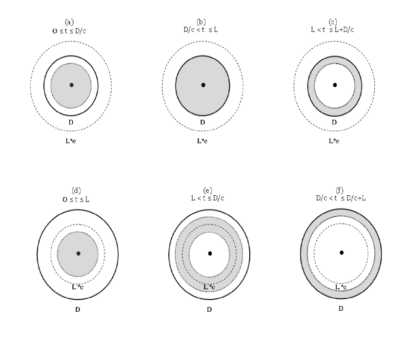
Figure 1: Areas of coverage for the propagation of an expanding signal. (a)-(c) assumes $D<Lc$, (d)-(f) assumes $D>Lc$. The shaded portion is the relative area being swept by the signal.

(a)	$\frac{1}{3}\pi\frac{D^{4}}{c}$
(b)	$\frac{4}{3}\pi D^{3}L-\frac{4}{3}\pi\frac{D^{4}}{c}$
(c)	$\pi\frac{D^{4}}{c}$
(d)	$\frac{1}{3}\pi L^{4}c^{3}$
(e)	$\frac{4}{3}\pi c^{3}L\left[\frac{D^{3}}{c^{3}}-\frac{3}{2}\frac{D^{2}L}{c^{2}}+\frac{L^{2}D}{c}-\frac{1}{2}L^{3}\right]$
(f)	$\frac{4}{3}\pi D^{3}L-\frac{1}{3}\pi L^{4}c^{3}$

Table 1: The equations corresponding to the different expanding coverages of the signals in figure 1. Note the first terms in (a) and (d) correspond to the lightcone from the origin to $D$ and $L$ respectively.

In table 1 are the equations for $V*t$ for images a-f in figure 1. Both sets of equations give the same value in the case $Lc=D$.

Now in order to integrate these with the Drake equation, we modify the equation to calculate the average CC density. This is the expected number of CCs per unit space. We do this by changing the term, $R^{*}$ to become $r^{*}$, the stellar creation rate per unit volume. Therefore, we can calculate the expected communicative civilization density as

$$n=r^{*}f_{s}L$$ (4)

However, when trying to calculate the number of CCs that can detect a signal, we replace $L$ with the volume-time to get

$$N=r^{*}f_{s}\sum^{t_{f}}_{0}V*t$$ (5)

where a contact is made with almost certainty if $N\geq 1$. Volume-time is represented by the following for $Lc>D$ and $Lc<D$

$$\frac{1}{3}\pi\frac{D^{4}}{c}+\frac{4}{3}\pi D^{3}L-\frac{4}{3}\pi\frac{D^{4}}{c}+\pi\frac{D^{4}}{c}$$ (6)

$$\frac{1}{3}\pi L^{4}c^{3}+\frac{4}{3}\pi c^{3}L\left[\frac{D^{3}}{c^{3}}-\frac{3}{2}\frac{D^{2}L}{c^{2}}+\frac{L^{2}D}{c}-\frac{1}{2}L^{3}\right]+\frac{4}{3}\pi D^{3}L-\frac{1}{3}\pi L^{4}c^{3}$$ (7)

The first and final terms in each equation cancel giving

$$\frac{4}{3}\pi D^{3}L$$ (8)

$$\frac{2}{3}\pi L\left[4D^{3}-3D^{2}Lc+2L^{2}Dc^{2}-c^{3}L^{3}\right]$$ (9)

3 Communicative civilization density and contact

Taking equations 4 and 5 into account, the question naturally arises of how the density of CC affects the probability of contact. Solving for $r^{*}f_{s}$ in 4, two variables that are otherwise extremely difficult to estimate, and changing equation 5 we can see that

$$N=\frac{n}{L}\sum^{t_{f}}_{0}V*t$$ (10)

We now have a probability of a signal being detected by another CC only in terms of the average CC density in the region considered, the average lifetime of a CC, and the volume-time which implicitly incorporates the maximum distance, $D$. For $Lc>D$ and $Lc<D$, $N$ follows as

$$N=\frac{4}{3}\pi nD^{3}$$ (11)

$$N=\frac{2}{3}\pi n\left[4D^{3}-3D^{2}Lc+2L^{2}Dc^{2}-c^{3}L^{3}\right]$$ (12)

In the first case of $Lc>D$ the number of CCs contacted depends only on the signal horizon distance and is independent of the lifetime of the civilization. In short, it is the expected number of CCs in the volume of space specified by the signal horizon distance. Where $Lc<D$, there is a more complex relationship where the broadcasting CC lifetime is an important factor. Given a threshold of $N=1$, we can thus derive any of the variables if two others are known. In particular, given assumptions on the average lifetime of CCs and the average detectable distance of their signals, we can estimate the minimum CC density and for a given volume, the minimum number of CCs necessary to make communication probable.

Using a basic measure of our galactic neighborhood as a sphere with a radius of 10,000 light years, figure 2 shows the number of CCs necessary for the CC density to be high enough to make contact likely within this volume. This assumes stars, habitable conditions, and CCs are distributed isotropically which is unlikely at best but a starting assumption. As expected, for CCs with very short lifetimes or very short signal horizons, the CC density must be massive to expect any contact. However, as CCs last longer and have signals with more durable range, the minimum density decreases hyperbolically until for high values of lifetime or signal horizons, only one other CC is necessary for contact to be probable.

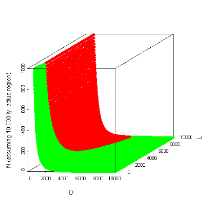
Figure 2: A graph of the minimum number of civilizations needed in a volume of radius 10,000 ly to make both contact (green and red area) and reciprocal contact (red area) likely based on $L$ and $D$.

What is most interesting about this analysis is that it demonstrates it can be possible for many CCs in the same galaxy to never contact one another. For example, even assuming the average CC has a lifetime of 1,000 years, ten times longer than Earth has been broadcasting, and has a signal horizon of 1,000 light-years, you need a minimum of 750 CCs in the galactic neighborhood to reach a minimum density. For example, if there were only 200 CCs in our galactic neighborhood roughly meeting these parameters, probabilistically they will never be aware of each other. The restriction of $D$ of 1,000 light-years is probably too conservative since under our current technology, the Arecibo observatory can detect a signal of its same broadcasting strength at 1,000 light-years. For the same $L$, increasing $D$ to 2,000 reduces the minimum number to 65 and increasing $D$ to 5,000 reduces it down to 3, though the signals would likely be received after the demise of the broadcasting CC.

These findings can give pause to both those who predict no other CCs or those who predict a high number of CCs in our galactic neighborhood. Arguing that the lack of contact signifies the lack of CCs may be tempered with the fact that if there is a signal horizon, even a galaxy replete with life may have relatively isolated CCs in the absence of interstellar travel or extremely power signals. On the other hand, high estimates of CCs in our galactic neighborhood does not guarantee that there will ever be contact between them, especially reciprocal.

Reciprocal contact can be estimated. On average, the signal needs to reach a volume of space of $1/n$ to reach another CC. The average distance between CCs and the average time to reach another CC can be derived from the two equations

$$\frac{1}{n}=\frac{4}{3}\pi(r)^{3}$$ (13)

$$\frac{1}{n}=\frac{4}{3}\pi(ct)^{3}$$ (14)

In [8] Duric and Field also calculate the average density of civilizations based on a time available for intelligible contact and come up with an average distance between CCs quantitatively similar to equation 13 where $r\approx\frac{1}{n^{1/3}}$. If $2t\leq L$ then reciprocal contact is likely on average assuming a CC immediately detects a signal on arrival and immediately sends a response back which arrives before the first CC dies out. This predicts a broadly social universe where, much like the old American public television children’s show Mr. Rogers’ Neighborhood, everyone knows their neighbor. However, in time $t$ both CCs could be aware of each other though they have not yet communicated.

3.1 Estimating D

Estimations of $D$ are necessarily bound to considerations of broadcasting and receiver abilities that would dictate an average distance for intentionally or unintentionally broadcast signals to be received. A proper estimate of $D$ would necessarily depend on the broadcast frequency, bandwidth of the signal, broadcast power, and both the transmitting and receiving antenna sizes. In [9], a range equation for a signal is presented of the form

$$\frac{\eta_{T}\eta_{R}d_{t}^{2}d_{r}^{2}P_{t}}{\lambda^{2}R^{2}}=2\times 10^{3}k_{D}k_{R}T\left(\frac{B}{\tau}\right)^{1/2}$$ (15)

where $\eta_{T}$ and $\eta_{R}$ are the aperture efficiencies of the transmitting and receiving antennas with diameters of $d_{t}$ and $d_{r}$ respectively. $P_{t}$ is the radiated transmitter broadcast power (megawatts), $\lambda$ is the broadcast wavelength (meters), $R$ is the maximum range (light-years), $k_{D}$ and $k_{R}$ are the detection efficiency and receiver efficiency factors, $T$ is the system noise (kelvin), $B$ is the bandwidth (hertz), and $\tau$ is the integration time needed to detect the signal (seconds). By estimating some of the constants and and realizing the maximum $\tau$ is $L$, you can derive a minimum necessary broadcast power for a given $D$ or estimate $D$ for an assumed broadcast power. You can also estimate upper limits for bandwidth and minimum antenna sizes. For example, using the estimates for the variables in [9] of $\eta_{T}=\eta_{R}$=0.6, $k_{D}$=5, $k_{R}$=2,$T=20^{\circ}$K, $d_{r}=d_{t}$=26 m and assuming a bandwidth of 1 kHz at a $\lambda$ of 12 cm for $D$ of 1,000 ly and $L$ of 1,000 years we would need a minimum broadcast power of 6.2 MW, assuming integration time is the full life of the CC, which is probably far too large of an estimate.

4 Conclusion

The Drake Equation, almost five decades after its debut, remains as controversial and inconclusive as it was at its inception. A good viewpoint is raised in [10] that discusses the problem that the Drake equation should not be viewed as an exact mathematical equation, especially since it includes both astronomical variables such as star formation rate and planet abundance, biological variables such as the probability for the emergence of life, as well as more socioeconomic variables such as the probability for the development of civilization and advanced communication. There is no way to find a ‘right’ value for these variables.

However, the search for extraterrestrial life need not suffer because of no immediate obvious contact despite high estimates of life in our galaxy and universe. Under appropriate considerations, if the density of life is lower than a certain threshold and assuming colonization driven contact is unlikely, communicating civilizations could remain completely ignorant of each other. Of course these strict constraints can be circumvented by interstellar travel or permanent automatic beacons. This paper has attempted to add some additional considerations to the Drake equation which will allow us to more feasibly estimate the conditions under which we can hope to eventually discover we are not alone.

References

- [1] The Fermi Paradox is based on a possibly apocryphal question Enrico Fermi supposedly asked at Los Alamos in the 1940s: given that it seems there is a high probability for the evolution of intelligent life, why haven’t we found it?
- [2] Drake, FD, Discussion at Space Science Board, National Academy of Sciences Conference on Extraterrestrial Intelligent Life, (1961)
- [3] Shklovskii, IS & Sagan, C, Intelligent life in the universe, New York: Dell, (1966)
- [4] Kreifeldt, JG, “A formulation for the number of communicative civilizations in the galaxy”, Icarus, 14, pp.419-430, (1971)
- [5] Wallenhorst, SG, “The Drake Equation reexamined”, Quar. J. of the Royal Astron. Soc. , 22, pp.380-387, (1981)
- [6] Tipler, FJ, “Extraterrestrial intelligent beings do not exist”, Quar. J. of the Royal Astron. Soc., 21, pp.267-281 (1980)
- [7] Cirkovic, MM, “The Temporal Aspect of the Drake Equation and SETI”, Astrobiology, 4, pp.225-231 (2004)
- [8] Duric, N & Field, L, “On the detectability of intelligent civilizations in the galaxy”, Serb. Astron. J., 167, pp.1-10 (2003)
- [9] Kuiper, TBH & Morris, M, “Searching for extraterrestrial civilizations”, Science, 196, pp.616-621 (1977)
- [10] Burchell, MJ, “W(h)ither the Drake Equation?”, Intl. J. of Astrobiology, 5, pp.243-250, (2006)