Excitation spectrum and effective interactions of highly-elongated Fermi gas

Abstract

Full 3D calculations of small two-component Fermi gases under highly-elongated confinement, in which unlike fermions interact through short-range potentials with variable atom-atom $s$-wave scattering length, are performed using the correlated Gaussian approach. In addition, microscopic 1D calculations are performed for effective “atomic” and “molecular” 1D model Hamiltonian. Comparisons of the 3D and 1D energies and excitation frequencies establish the validity regimes of the effective 1D Hamiltonian. Our numerical results for three- and four-particle systems suggest that the effective 1D atom-dimer and dimer-dimer interactions are to a good approximation determined by simple analytical expressions. Implications for the description of quasi-1D Fermi gases within strict 1D frameworks are discussed.

I Introduction

Ultracold atomic and molecular gases are considered nearly ideal model systems since their confining geometry, size and interaction strength can be varied with unprecedented control review . A key goal of ongoing research activities is to experimentally determine the complete phase diagram of cold atom systems science . The successful demonstration of this task would provide a first step towards utilizing cold atom systems as quantum emulators. The determination of phase diagrams of quasi-1D systems has received considerable attention since these systems can, under certain circumstances, be described by 1D model Hamiltonian whose properties have been studied extensively in the literature 1dexact . For this class of systems, the challange is to establish which aspects of quasi-1D cold atom experiments can be described by 1D model Hamiltonian.

Naively, the 1D scattering strength between two particles in a wave guide geometry may be estimated by integrating out the tightly-confined transverse degrees of freedom. However, while the result is accurate in the weakly-interacting regime, Olshanii’s seminal work olsh98 shows that the 1D scattering strength $g_{\mathrm{1D}}^{\mathrm{aa}}$ depends in general non-trivially on the 3D $s$-wave atom-atom scattering length $a_{\mathrm{3D}}^{\mathrm{aa}}$ and the transverse angular frequency $\omega_{\rho}$. The coupling constant $g_{\mathrm{1D}}^{\mathrm{aa}}$ determined by Olshanii is now widely used in many-body studies of Bose and Fermi gases. The applicability of an effective atomic 1D Hamiltonian whose two-body interactions are parameterized in terms of $g_{\mathrm{1D}}^{\mathrm{aa}}$ has, e.g., been confirmed for a Bose gas under highly elongated harmonic confinement by comparing the results of 3D and 1D Monte Carlo calculations astr04 .

Over the past few years, an effective atomic 1D Hamiltonian has also been applied extensively to two-component Fermi gases under highly-elongated confinement 1dpolarized ; toka04fuch04 ; mora05 ; in this case, however, the validity regime of the effective atomic 1D Hamiltonian has not yet been assessed carefully. It is clear that an effective atomic 1D Hamiltonian description breaks down when tightly-bound molecules form. In this case, the system may be described by an effective molecular 1D Hamiltonian that treats each tightly-bound molecule as a composite boson. While the functional form of such an effective molecular Hamiltonian is generally agreed upon, the parametrization of the effective atom-dimer and dimer-dimer interactions varies toka04fuch04 ; mora05 . Furthermore, it is not clear whether or not the effective atomic and molecular 1D Hamiltonian descriptions connect smoothly in the strongly-interacting regime.

This work presents 3D and 1D zero-temperature ab initio calculations for small two-component Fermi gases with up to $N=4$ atoms under highly-elongated confinement and assesses the validity regimes of effective atomic and molecular 1D Hamiltonian. Our main findings are: i) The 3D energies are reproduced well by an effective atomic 1D Hamiltonian for small $|a_{\mathrm{3D}}^{\mathrm{aa}}/a_{\rho}|$ ($a_{\mathrm{3D}}^{\mathrm{aa}}<0$), where $a_{\rho}$ denotes the oscillator length in the tight confinement direction [see Eq. (5)]. ii) For small positive $a_{\mathrm{3D}}^{\mathrm{aa}}/a_{\rho}$, the 3D energies are reproduced well by an effective molecular 1D Hamiltonian that depends on the effective 1D atom-dimer and dimer-dimer scattering lengths $a_{\mathrm{1D}}^{\mathrm{ad}}$ and $a_{\mathrm{1D}}^{\mathrm{dd}}$; analytical expressions for $a_{\mathrm{1D}}^{\mathrm{ad}}$ and $a_{\mathrm{1D}}^{\mathrm{dd}}$ are presented. iii) For two of the energy curves considered (see below), the descriptions based on the effective atomic and molecular 1D Hamiltonian join fairly smoothly in the strongly-interacting regime, defined through $|a_{\mathrm{3D}}^{\mathrm{aa}}|\gtrsim a_{\rho}$; not surprisingly, the dependence of the energies on the aspect ratio is largest in the strongly-interacting regime.

Our assessment of the validity regimes of the effective atomic and molecular 1D Hamiltonian for small systems is expected to provide guidelines for larger systems, and is thus of great importance for realizing condensed matter and materials analogs as well as for exploiting cold atom systems for quantum computation and quantum simulation. Quasi-1D few-fermion systems can be prepared by loading a gas of ultracold fermions into an optical lattice lattice . Measurements of the excitation spectrum as a function of the interaction strength would provide a stringent test of our microscopic predictions.

Section II introduces the 3D model Hamiltonian, discusses the numerical techniques employed to solve the corresponding Schrödinger equation and presents the resulting 3D energies. Section III introduces the effective atomic and molecular 1D Hamiltonian and presents detailed comparisons between the 3D and 1D energies. Section IV discusses the excitation spectrum of strongly-interacting two-component Fermi gases under highly-elongated cylindrically-symmetric confinement. Finally, Sec. V concludes.

II Full 3D Treatment: Energetics

This section introduces the 3D model Hamiltonian and the numerical techniques employed to solve the corresponding Schrödinger equation. 3D energies are presented for $N=2-4$ fermions under highly-elongated confinement.

Our 3D model Hamiltonian $H_{\mathrm{3D}}$ for the trapped two-component Fermi gas with $N_{1}$ spin-up and $N_{2}$ spin-down fermions, where $N=N_{1}+N_{2}$, reads

$$H_{\mathrm{3D}}=\sum_{i=1}^{N}\left[\frac{-\hbar^{2}}{2m}\nabla^{2}_{\vec{r}_{i}}+V_{\mathrm{tr}}(\vec{r}_{i})\right]+\sum_{i=1}^{N_{1}}\sum_{j=N_{1}+1}^{N}V_{\mathrm{tb}}({r}_{ij}).$$ (1)

Here, $m$ and $\vec{r}_{i}$ denote the atom mass and the position vector of the $i$th atom, $\vec{r}_{i}=(x_{i},y_{i},z_{i})$. The trapping potential $V_{\mathrm{tr}}(\vec{r}_{i})$ is given by

$$V_{\mathrm{tr}}(\vec{r}_{i})=\frac{1}{2}m\omega_{z}^{2}(\lambda^{2}\rho_{i}^{2}+z_{i}^{2}),$$ (2)

where $\rho_{i}$ and $\lambda$ are defined through $\rho_{i}=\sqrt{x_{i}^{2}+y_{i}^{2}}$ and

$$\omega_{\rho}=\lambda\omega_{z},$$ (3)

and $\omega_{\rho}$ and $\omega_{z}$ denote the transverse and axial angular frequencies. Unlike atoms interact through a spherically symmetric short-range Gaussian potential $V_{\mathrm{tb}}$,

$$V_{\mathrm{tb}}(r_{ij})=-V_{0}\exp\left(-\frac{r_{ij}^{2}}{2r_{0}^{2}}\right),$$ (4)

where ${r}_{ij}=|\vec{r}_{i}-\vec{r}_{j}|$. We take the range $r_{0}$ to be much smaller than the oscillator lengths $a_{z}$ and $a_{\rho}$ in the $z$- and $\rho$-directions,

$$a_{z,\rho}=\sqrt{\frac{\hbar}{m\omega_{z,\rho}}},$$ (5)

and adjust the depth $V_{0}$ ($V_{0}>0$) so that the free-space 3D $s$-wave atom-atom scattering length $a_{\mathrm{3D}}^{\mathrm{aa}}$ takes the desired value. A solid line in Fig. 1

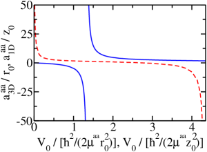
Figure 1: (Color online) The solid and dashed lines show the free-space scattering lengths $a_{\mathrm{3D}}^{\mathrm{aa}}$ and $a_{\mathrm{1D}}^{\mathrm{aa}}$ for the Gaussian potential $V_{\mathrm{tb}}$ as a function of the well depth $V_{0}$. The scattering lengths and depths are measured in the “natural units” of the free-space system, i.e., in units of $r_{0}$ [$z_{0}$] and $\hbar^{2}/(2\mu^{\mathrm{aa}}r_{0}^{2})$ [$\hbar^{2}/(2\mu^{\mathrm{aa}}z_{0}^{2})$] for the 3D [1D] system, where $\mu^{\mathrm{aa}}$ denotes the reduced mass of the atom-atom system.

shows $a_{\mathrm{3D}}^{\mathrm{aa}}$ as a function of the well depth $V_{0}$. To realize different negative $a_{\mathrm{3D}}^{\mathrm{aa}}$, we start with a non-interacting (NI) system ($V_{0}=0$) and increase the depth $V_{0}$ till $|a_{\mathrm{3D}}^{\mathrm{aa}}|$ becomes infinitely large; at this point, the free-space two-particle system supports a single zero-energy $s$-wave bound state. To realize different positive $a_{\mathrm{3D}}^{\mathrm{aa}}$, we increase $V_{0}$ further. In general, $V_{\mathrm{tb}}$ can lead not only to $s$-wave scattering but also to higher partial wave scattering. We have checked that the generalized $p$-wave scattering length and generalized scattering lengths corresponding to other higher partial waves are negligible over the range of well depths considered in this paper. This implies that $H_{\mathrm{3D}}$ effectively describes an $s$-wave interacting system.

To solve the time-independent Schrödinger equation for $H_{\mathrm{3D}}$, we separate off the center-of-mass motion and numerically solve the resulting Schrödinger equation in the relative coordinates. For $N_{1}=N_{2}=1$, we expand the relative wave function in terms of two-dimensional B-splines and diagonalize the Hamiltonian matrix. For the three- and four-particle systems, we employ a correlated Gaussian (CG) approach cgbook ; cgother that expands the relative wave function $\psi$ in terms of Gaussian basis functions $f_{k}^{(\rho)}f_{k}^{(z)}$,

$$\psi=\sum_{k=1}^{N_{b}}c_{k}{\cal{A}}$$

$$\left[f_{k}^{(\rho)}(\rho_{12},\cdots,\rho_{N-1,N})f_{k}^{(z)}(z_{12},\cdots,z_{N-1,N})\right],$$ (6)

where

$$f_{k}^{(\rho)}(\rho_{12},\cdots,\rho_{N-1,N})=\exp\left[-\sum_{i<j}^{N}\left(\frac{\rho_{ij}}{\sqrt{2}d_{ij,k}^{(\rho)}}\right)^{2}\right]$$ (7)

and $f_{k}^{(z)}$ is defined analogously. The relative coordinates $\rho_{ij}$ and $z_{ij}$ are defined as $\rho_{ij}=\sqrt{(x_{i}-x_{j})^{2}+(y_{i}-y_{j})^{2}}$ and $z_{ij}=z_{i}-z_{j}$ ($i,j=1,\cdots,N$ with $i<j$). The widths $d_{ij,k}^{(\rho)}$ and $d_{ij,k}^{(z)}$ are chosen semi-stochastically for each pair $ij$ and $k$th basis function, and the total number of basis functions is denoted by $N_{b}$. In Eq. (II), the $c_{k}$ denote expansion coefficients and ${\cal{A}}$ denotes an anti-symmetrizer that ensures the proper symmetry of the two-component Fermi gas under exchange of identical fermions. For $N=3$ ($N_{1}=2$ and $N_{2}=1$), ${\cal{A}}$ can be conveniently written as $1-P_{12}$, where $P_{12}$ permutes the two up-fermions. For $N=4$ ($N_{1}=N_{2}=2$), ${\cal{A}}$ can be written as $1-P_{12}-P_{34}+P_{12}P_{34}$.

For the interaction and confining potentials chosen, the Hamiltonian and overlap matrix elements (the basis functions $f_{k}^{(\rho)}f_{k}^{(z)}$ do not form an orthogonal set) can be constructed analytically. The diagonalization of the eigenvalue equation is then performed using standard techniques. The resulting eigenenergies, whose accuracy can be systematically improved by increasing the number of basis functions and by optimizing the widths $d_{ij,k}^{(\rho)}$ and $d_{ij,k}^{(z)}$ of the Gaussian functions, provide upper bounds to the exact eigenenergies.

The 2D functions $f_{k}^{(\rho)}$ are eigenfunctions of the $z$-component $L_{z}$ of the orbital angular momentum operator with eigenvalues $\hbar m_{l}$, $m_{l}=0$ cgbook , while the 1D functions $f_{k}^{(z)}$ have even parity $P_{z}=+1$. For the $N=4$ system, the energetically lowest-lying state has $m_{l}=0$ and $P_{z}=+1$ for all 3D scattering lengths $a_{\mathrm{3D}}^{\mathrm{aa}}$ and the basis functions $f_{k}^{(\rho)}f_{k}^{(z)}$ defined in and below Eq. (II) have the proper symmetry. The ground state of the NI $N=3$ system, in contrast, has $m_{l}=0$ and odd parity ($P_{z}=-1$), which cannot be described by the basis functions $f_{k}^{(\rho)}f_{z}^{(z)}$. To describe states with odd parity, we add a spectator atom that does not interact with the $N$-fermion system of interest; the energy of the NI spectator atom follows from its $m_{l}$ quantum number and from its parity, and is subtracted at the end of the calculation. Since the basis functions of the $(N+1)$-system have even parity, the spectator atom and the $N$-fermion system either both have even parity or both have odd parity. In the following, we label our solutions by the parity $P_{z}$; if a spectator atom is added for computational purposes, we report the parity of the physical system of interest. Furthermore, since all energetically lowest-lying states of two-component Fermi gases under highly-elongated confinement have $m_{l}=0$, we frequently omit the $m_{l}$ label.

Figures 2(a) and (b) show the relative 3D energies for $N=2-4$

Figure 2: (Color online) Relative 3D energies calculated using $H_{\mathrm{3D}}$ as a function of $a_{\rho}/a_{\mathrm{3D}}^{\mathrm{aa}}$ for (a) negative $a_{\mathrm{3D}}^{\mathrm{aa}}$ and (b) positive $a_{\mathrm{3D}}^{\mathrm{aa}}$ for $\lambda=10$ [$r_{0}=0.03a_{z}$ for $a_{\mathrm{3D}}^{\mathrm{aa}}<0$ and $N=4$, and $0.01a_{z}$ otherwise]. Solid lines show the $s$-wave energy $E_{s}(1,1)-E_{\mathrm{CM},0}$ of the two-particle system, dashed lines show the lowest three-particle energy $E(2,1)-E_{\mathrm{CM},0}$ with $P_{z}=-1$, dotted lines show the lowest three-particle energy $E(2,1)-E_{\mathrm{CM},0}$ with $P_{z}=+1$ and dash-dotted lines show one half of the lowest four-particle energy $E(2,2)-E_{\mathrm{CM},0}$ with $P_{z}=+1$. The horizontal solid lines on the left side of panel (a) indicate the relative energies of the NI systems: $E_{s}(1,1)-E_{\mathrm{CM},0}=10.5\hbar\omega_{z}$, $E(2,1)-E_{\mathrm{CM},0}=22\hbar\omega_{z}$ ($P_{z}=-1$), $E(2,1)-E_{\mathrm{CM},0}=23\hbar\omega_{z}$ ($P_{z}=+1$), and $[E(2,2)-E_{\mathrm{CM},0}]/2=16.75\hbar\omega_{z}$.

and $\lambda=10$ as a function of the inverse 3D scattering length $a_{\rho}/a_{\mathrm{3D}}^{\mathrm{aa}}$. Solid lines in Figs. 2(a) and (b) show the relative $s$-wave ground state energy $E_{s}(1,1)-E_{\mathrm{CM},0}$ of the two-body system. For later convenience, the energy $E_{s}(1,1)$ as well as the energies $E(N_{1},N_{2})$ (see below) include the center-of-mass ground state energy $E_{\mathrm{CM},0}$, $E_{\mathrm{CM},0}=\hbar\omega_{\rho}+\hbar\omega_{z}/2$. In the NI limit, $E_{s}(1,1)-E_{\mathrm{CM},0}$ equals $10.5\hbar\omega_{z}=1.05\hbar\omega_{\rho}$. In the absence of the confining potential in the $z$-direction, the relative two-body energy is always smaller than $\hbar\omega_{\rho}$, indicating the existence of a quasi-1D bound state for all 3D scattering lengths $a_{\mathrm{3D}}^{\mathrm{aa}}$ olsh98 ; berg02 . The confining potential in the $z$-direction pushes the energy up; in the NI limit, the up-shift is given by the zero-point energy $\hbar\omega_{z}/2$.

For the $N=3$ system, the relative energies $E(2,1)-E_{\mathrm{CM},0}$ of the energetically lowest-lying states with $P_{z}=+1$ and $-1$ are shown by dotted and dashed lines, respectively. The $P_{z}=-1$ state has lower energy for small $|a_{\mathrm{3D}}^{\mathrm{aa}}|$, $a_{\mathrm{3D}}^{\mathrm{aa}}<0$ [see Fig. 2(a)], while the $P_{z}=+1$ state has lower energy for small positive $a_{\mathrm{3D}}^{\mathrm{aa}}$ [the crossover of the two states is not visible on the scale shown in Fig. 2(b); it occurs at $a_{\rho}/a_{\mathrm{3D}}^{\mathrm{aa}}\approx 2$ (see also Fig. 3)]. The relative three-particle energies are just slightly larger than the relative two-body $s$-wave energies in the limit of small positive $a_{\mathrm{3D}}^{\mathrm{aa}}$, indicating that the three-particle system can be thought of as consisting of an $s$-wave dimer and an unpaired atom. The relative ground state energy $E(2,2)-E_{\mathrm{CM},0}$ of the four-particle system has $P_{z}=+1$ for all 3D scattering lengths $a_{\mathrm{3D}}^{\mathrm{aa}}$; to ease comparisons between the energies of the two- and four-particle systems, dash-dotted lines in Figs. 2(a) and (b) show one half of the relative four-particle energy. For small positive $a_{\mathrm{3D}}^{\mathrm{aa}}$, the four-particle energy approaches approximately twice the energy of the two-particle system, indicating that the four-particle system can be thought of as consisting of two $s$-wave molecules. No tightly-bound trimers or tetramers are formed in the $a_{\mathrm{3D}}^{\mathrm{aa}}\rightarrow 0^{+}$ limit, in agreement with results for zero-range interactions petr03 ; petr04 ; moran3 .

The 3D energies can be combined to define the universal energy curve $\Lambda_{N_{1},N_{2}}$ for a two-component Fermi gas under external cylindrically symmetric confinement,

$$\Lambda_{N_{1},N_{2}}=\frac{E(N_{1},N_{2})-N_{\mathrm{d}}E_{s}(1,1)-N_{\mathrm{f}}\hbar(\omega_{\rho}+\frac{1}{2}\omega_{z})}{E_{\mathrm{NI}}(N_{1},N_{2})-N\hbar(\omega_{\rho}+\frac{1}{2}\omega_{z})},$$ (8)

where $N_{\mathrm{d}}=\min\{N_{1},N_{2}\}$ and $N_{\mathrm{f}}=|N_{1}-N_{2}|$. In Eq. (8), $E_{\mathrm{NI}}(N_{1},N_{2})$ denotes the energy of the NI system, and the energies $E_{\mathrm{NI}}(N_{1},N_{2})$, $E(N_{1},N_{2})$ and $E_{s}(1,1)$ include the center-of-mass ground state energy $E_{\mathrm{CM},0}$. To remove dependencies of the total energy $E(N_{1},N_{2})$ of the trapped system on $V_{\mathrm{tb}}$, the $s$-wave ground state energy $E_{s}(1,1)$ of the trapped two-particle system is subtracted on the right hand side of Eq. (8). If $E(N_{1},N_{2})$ corresponds to the energetically lowest-lying state of the NI system, the universal energy curve $\Lambda_{N_{1},N_{2}}$ equals one. Conversely, if $\Lambda_{N_{1},N_{2}}$ equals zero in the $a_{\mathrm{3D}}^{\mathrm{aa}}\rightarrow 0^{+}$ limit, then this indicates that the system is effectively NI and that induced interactions are absent. The definition of the universal energy curve presented in Eq. (8) for cylindrically-symmetric two-component Fermi systems constitutes a straightforward generalization of that previously introduced for spherically-symmetric two-component systems stec07b ; stec08 .

Figure 3

Figure 3: (Color online) $\Lambda_{N_{1},N_{2}}$ as a function of $a_{\rho}/a_{\mathrm{3D}}^{\mathrm{aa}}$: Panel (a) covers a large scattering length range while panel (b) shows an enlargement of the strongly-interacting regime. Thick dotted, dashed and solid lines show $\Lambda_{2,2}$ ($P_{z}=+1$), $\Lambda_{2,1}$ ($P_{z}=+1$) and $\Lambda_{2,1}$ ($P_{z}=-1$) calculated using $H_{\mathrm{3D}}$ for $\lambda=10$ [$r_{0}=0.03a_{z}$ for $a_{\mathrm{3D}}^{\mathrm{aa}}<0$ and $N=4$, and $0.01a_{z}$ otherwise]. Thin dash-dash-dotted and dash-dot-dotted lines show the corresponding 1D energy curves calculated using $H_{\mathrm{1D}}^{\mathrm{a}}$ and $H_{\mathrm{1D}}^{\mathrm{m}}$.

shows the 3D energy curves $\Lambda_{N_{1},N_{2}}$ as a function of $a_{\rho}/a_{\mathrm{3D}}^{\mathrm{aa}}$ for $\lambda=10$; the energies used to calculate the $\Lambda_{N_{1},N_{2}}$ are the same as those shown in Fig. 2. A thick dotted line shows $\Lambda_{2,2}$ calculated using the four-body energies $E(2,2)$ that correspond to states with $m_{l}=0$ and $P_{z}=+1$. The energy curve $\Lambda_{2,2}$ decreases monotonically from 1 to approximately 0 as $a_{\rho}/a_{\mathrm{3D}}^{\mathrm{aa}}$ increases from small negative to large positive values. Thick dashed and solid lines in Fig. 3 show the energy curves $\Lambda_{2,1}$ for the energetically lowest-lying $N=3$ states with $P_{z}=+1$ and $-1$, respectively. It can be seen that these $N=3$ energy curves cross at $a_{\rho}/a_{\mathrm{3D}}^{\mathrm{aa}}\approx 1.9$. For $a_{\mathrm{3D}}^{\mathrm{aa}}\rightarrow 0^{-}$ (NI limit), the ground state has $m_{l}=0$ and $P_{z}=-1$: One spin-up and one spin-down atom occupy the ground state harmonic oscillator orbital while the second up-atom occupies the first excited state harmonic oscillator orbital. For $a_{\mathrm{3D}}^{\mathrm{aa}}\rightarrow 0^{+}$, in contrast, the ground state for $N=3$ has $m_{l}=0$ and $P_{z}=+1$: The system consists of a tightly-bound dimer and an atom, which both occupy the lowest trap state. In this limit, the energy of the state with $P_{z}=-1$ is about $\hbar\omega_{z}$ larger than the energy of the $P_{z}=+1$ state [note that the energy difference is too small to be visible on the scale shown in Fig. 2(b)]. This suggests that the tightly-bound molecule and the unpaired atom interact through effective 1D potentials that lead to even and odd parity scattering for $P_{z}=+1$ and $-1$, respectively (see also the next section).

III 1D Treatment: Energetics and Effective Interactions

This section considers effective atomic and molecular 1D Hamiltonian, which assume that the motion in the $\rho$-direction is frozen, and compares the resulting 1D energies with the 3D energies discussed in the previous section. The applicability of the 1D model Hamiltonian and their parametrizations are discussed in detail.

If the system behaves like an atomic gas, the effective atomic 1D Hamiltonian $H_{\mathrm{1D}}^{\mathrm{a}}$ is given by

$$H_{\mathrm{1D}}^{\mathrm{a}}=\sum_{i=1}^{N}\left[\frac{-\hbar^{2}}{2m}\frac{\partial^{2}}{\partial z_{i}^{2}}+V_{\mathrm{tr}}(z_{i})\right]+\sum_{i=1}^{N_{1}}\sum_{j=N_{1}+1}^{N}V_{\mathrm{tb}}({z}_{ij}),$$ (9)

where

$$V_{\mathrm{tr}}(z_{i})=\frac{1}{2}m\omega_{z}^{2}z_{i}^{2}.$$ (10)

In Eq. (9), the spin-up and spin-down fermions interact through the two-body potential $V_{\mathrm{tb}}(z_{ij})$ and, as in the 3D Hamiltonian $H_{\mathrm{3D}}$ [see Eq. (1)], like atoms do not interact. The two-body potential $V_{\mathrm{tb}}$ is chosen such that its 1D even parity atom-atom scattering length $a_{\mathrm{1D}}^{\mathrm{aa}}$ is given by olsh98

$$a_{\mathrm{1D}}^{\mathrm{aa}}=-\frac{\hbar}{2\mu^{\mathrm{aa}}\omega_{\rho}}\left(\frac{1}{a_{\mathrm{3D}}^{\mathrm{aa}}}-1.4603\sqrt{\frac{\mu^{\mathrm{aa}}\omega_{\rho}}{\hbar}}\right),$$ (11)

where $\mu^{\mathrm{aa}}$ denotes the reduced mass of the atom-atom system. The 1D even parity scattering length $a_{\mathrm{1D}}^{\mathrm{aa}}$ [solid lines in Figs. 4(a) and (b)]

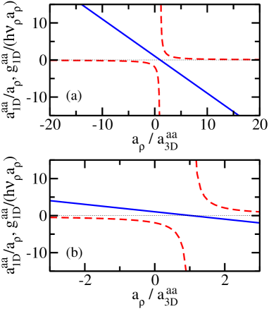
Figure 4: (Color online) 1D even parity atom-atom scattering length $a_{\mathrm{1D}}^{\mathrm{aa}}/a_{\rho}$ (solid line) and corresponding 1D scattering strength $g_{\mathrm{1D}}^{\mathrm{aa}}/(\hbar\omega_{\rho}a_{\rho})$ (dashed line) as a function of the inverse 3D atom-atom scattering length $a_{\rho}/a_{\mathrm{3D}}^{\mathrm{aa}}$: Panel (a) covers a large 3D scattering length range while panel (b) shows an enlargement of the strongly-interacting regime. The 1D coupling constant $g_{\mathrm{1D}}^{\mathrm{aa}}$ changes from about $-\hbar\omega_{\rho}a_{\rho}$ to about $-60\hbar\omega_{\rho}a_{\rho}$ as $a_{\rho}/a_{\mathrm{3D}}^{\mathrm{aa}}$ increases from $-1$ to $1$ (i.e., in the strongly-interacting regime).

is large for large $|a_{\rho}/a_{\mathrm{3D}}^{\mathrm{aa}}|$ ($a_{\mathrm{3D}}^{\mathrm{aa}}<0$), decreases linearly with increasing $a_{\rho}/a_{\mathrm{3D}}^{\mathrm{aa}}$, and crosses zero at $a_{\rho}/a_{\mathrm{3D}}^{\mathrm{aa}}=1.0326$. Since the 1D coupling constant $g_{\mathrm{1D}}^{\mathrm{aa}}$,

$$g_{\mathrm{1D}}^{\mathrm{aa}}=-\frac{\hbar^{2}}{\mu^{\mathrm{aa}}a_{\mathrm{1D}}^{\mathrm{aa}}},$$ (12)

diverges when $a_{\mathrm{1D}}^{\mathrm{aa}}$ vanishes, the quasi-1D system is infinitely strongly-interacting for a finite $a_{\mathrm{3D}}^{\mathrm{aa}}$. Furthermore, a large positive $a_{\mathrm{1D}}^{\mathrm{aa}}$ indicates the presence of a weakly-bound even parity two-body bound state. In the literature, the effective 1D atom-atom potential $V_{\mathrm{tb}}$ is frequently modeled by a 1D zero-range $\delta$-function potential. For numerical convenience, we use instead a 1D Gaussian potential [Eq. (4) with $r_{ij}$ and $r_{0}$ replaced by $z_{ij}$ and $z_{0}$] with a small width $z_{0}$ ($z_{0}=0.005a_{z}$) and a depth adjusted so as to obtain the desired $a_{\mathrm{1D}}^{\mathrm{aa}}$. We have checked that the resulting 1D energies depend only very weakly on $z_{0}$ and that the odd parity atom-atom scattering length is negligibly small over the range of well depths considered. The 1D even parity atom-atom scattering length $a_{\mathrm{1D}}^{\mathrm{aa}}$ for the 1D Gaussian potential is shown in Fig. 1 by a dashed line as a function of the well depth $V_{0}$.

For the 3D energy curves considered in Fig. 3, the effective atomic 1D Hamiltonian is expected to provide an accurate description if the size of the 1D dimer is much larger than the oscillator length $a_{\rho}$ (see, e.g., Ref. toka04fuch04 ). Approximating the size of the dimer by $|a_{\mathrm{1D}}^{\mathrm{aa}}|$ and using $|a_{\mathrm{1D}}^{\mathrm{aa}}|\approx|a_{\rho}^{2}/a_{\mathrm{3D}}^{\mathrm{aa}}|$ [i.e., using the first part on the right hand side of Eq. (11)], the validity condition $a_{\rho}\gg|a_{\mathrm{3D}}^{\mathrm{aa}}|$ is obtained. Relaxing the disparity of length scales, we have $a_{\rho}\gtrsim|a_{\mathrm{3D}}^{\mathrm{aa}}|$ with $a_{\mathrm{3D}}^{\mathrm{aa}}<0$.

To obtain the 1D energies of the effective atomic 1D Hamiltonian $H_{\mathrm{1D}}^{\mathrm{a}}$, we first separate off the center-of-mass motion and then solve the resulting Schrödinger equation in the relative coordinates using the B-spline approach for the two-particle system and the CG approach for the three- and four-particle systems. Our CG implementation for the 1D system parallels that discussed above for the 3D system. The main difference is that the basis functions are now given by $f_{k}^{(z)}$ instead of by $f_{k}^{(\rho)}f_{k}^{(z)}$. Systems with odd parity are, similarly to the 3D case, treated by adding a NI spectator atom. For large positive $a_{\mathrm{1D}}^{\mathrm{aa}}$, we find that the energetically lowest-lying 1D states accurately model the corresponding 3D states. For small positive $a_{\mathrm{1D}}^{\mathrm{aa}}$, however, the effective atomic 1D Hamiltonian supports a sequence of tightly-bound three- and four-particle states, which have no analog in the 3D system (as discussed above, tightly-bound three- and four-particle states are not supported by $H_{\mathrm{3D}}$); these 1D states are excluded from our analysis. The 1D energy states of interest to us are those that smoothly evolve from a NI gas-like state in the $a_{\mathrm{1D}}^{\mathrm{aa}}\rightarrow\infty$ limit to states that describe a weakly-bound molecule and an atom or two weakly-bound molecules for $N=3$ and $N=4$, respectively, in the $a_{\mathrm{1D}}^{\mathrm{aa}}\rightarrow 0^{+}$ limit. Our last 1D energies are reported for $a_{\rho}/a_{\mathrm{3D}}^{\mathrm{aa}}\approx 1$ for $N=3$ with $P_{z}=+1$, and for $a_{\rho}/a_{\mathrm{3D}}^{\mathrm{aa}}=0$ for $N=3$ with $P_{z}=-1$ and $N=4$ with $P_{z}=+1$. We note that tightly-bound $N$-body states also exist for negative $a_{\mathrm{1D}}^{\mathrm{aa}}$. Their existence can be traced back to the finite range of the Gaussian two-body interaction potential; an effective atomic 1D Hamiltonian with zero-range $\delta$-function potentials and negative $a_{\mathrm{1D}}^{\mathrm{aa}}$ does not support tightly-bound $N$-body states.

The 1D energies determine the 1D energy curves $\Lambda_{N_{1},N_{2}}$, which are given by Eq. (8) with $\omega_{\rho}=0$, $E_{s}(1,1)$ denoting the 1D even parity two-particle energy, and $E(N_{1},N_{2})$ and $E_{\mathrm{NI}}(N_{1},N_{2})$ interpreted as 1D energies. Thin dash-dash-dotted lines in Fig. 3 show the 1D energy curves obtained using $H_{\mathrm{1D}}^{\mathrm{a}}$ for $N=3$ and 4. The agreement between the 1D energy curves and the corresponding 3D quantities (thick lines) in the weakly-attractive regime is excellent. For $P_{z}=+1$, the agreement between the 1D and 3D energy curves extends into the strongly-interacting, large positive $a_{\mathrm{3D}}^{\mathrm{aa}}$ regime. The 1D energy curve for $N=3$ with $P_{z}=-1$, in contrast, starts deviating from the corresponding 3D energy curve for somewhat less strong interactions ($|a_{\rho}/a_{\mathrm{3D}}^{\mathrm{aa}}|\lesssim 2$ with $a_{\mathrm{3D}}^{\mathrm{aa}}<0$). We have checked that these deviations are not due to the finite range of $V_{\mathrm{tb}}$.

In addition to an effective atomic 1D Hamiltonian $H_{\mathrm{1D}}^{\mathrm{a}}$, we consider an effective molecular 1D Hamiltonian $H_{\mathrm{1D}}^{\mathrm{m}}$. We show in the following that the 3D energy curves with $P_{z}=+1$ can be reproduced well for $a_{\mathrm{3D}}^{\mathrm{aa}}>0$ by treating the $N=3$ and 4 systems as effective two-particle systems that consist of an atom and a tightly-bound molecule and of two tightly-bound molecules, respectively. To this end, we model the atom-dimer and dimer-dimer interactions through a $\delta$-function potential. The effective two-particle 1D Hamiltonian for the relative coordinate $z$ then reads

$$H_{\mathrm{1D}}^{\mathrm{m}}=\frac{-\hbar^{2}}{2\mu^{j}}\frac{d^{2}}{dz^{2}}+\frac{1}{2}\mu^{j}\omega_{z}^{2}z^{2}+g_{\mathrm{1D}}^{j}\delta(z),$$ (13)

where $j={\mathrm{ad}}$ and $\mathrm{dd}$ for the atom-dimer and dimer-dimer system, respectively, and where the 1D coupling strengths $g_{\mathrm{1D}}^{\mathrm{ad}}$ and $g_{\mathrm{1D}}^{\mathrm{dd}}$ are related to the 1D scattering lengths $a_{\mathrm{1D}}^{\mathrm{ad}}$ and $a_{\mathrm{1D}}^{\mathrm{dd}}$ [Eq. (12) with $\mathrm{aa}$ replaced by $\mathrm{ad}$ and $\mathrm{dd}$, respectively]. We approximate the effective 1D atom-dimer and dimer-dimer scattering lengths $a_{\mathrm{1D}}^{\mathrm{ad}}$ and $a_{\mathrm{1D}}^{\mathrm{dd}}$ by the right hand side of Eq. (11) with superscripts aa replaced by ad and dd, respectively. The 3D atom-dimer and dimer-dimer scattering lengths $a_{\mathrm{3D}}^{\mathrm{ad}}$ and $a_{\mathrm{3D}}^{\mathrm{dd}}$, in turn, are approximated by their free-space values skor56 ; petr03 ; moran3 ; stec08 ,

$$a_{\mathrm{3D}}^{\mathrm{ad}}=1.18a_{\mathrm{3D}}^{\mathrm{aa}}$$ (14)

and petr04 ; stec07b ; stec08

$$a_{\mathrm{3D}}^{\mathrm{dd}}=0.608a_{\mathrm{3D}}^{\mathrm{aa}}.$$ (15)

Physically, this implies that molecules are formed in 3D and that their effective 3D interactions with atoms and other molecules are renormalized by the quasi-1D confinement.

The validity regime of the effective molecular 1D Hamiltonian $H_{\mathrm{1D}}^{\mathrm{m}}$ is expected to be determined by three conditions: i) Since the 3D free-space atom-dimer and dimer-dimer scattering lengths are derived assuming that $a_{\mathrm{3D}}^{\mathrm{aa}}\gg r_{0}$, the above parametrization is expected to break down when $a_{\mathrm{3D}}^{\mathrm{aa}}$ approaches $r_{0}$. ii) For three- and four-particle systems under spherically symmetric confinement, it has been shown stec08 that the full 3D energies on the BEC side (positive $a_{\mathrm{3D}}^{\mathrm{aa}}$) are well described by effective 3D atom-molecule and molecule-molecule models if $a_{\mathrm{3D}}^{\mathrm{aa}}$ is much smaller than the harmonic oscillator length. Correspondingly, since our parametrization of the effective interactions given in Eqs. (13)-(15) for the highly-elongated system assumes that the molecules are formed in 3D, the validity regime of $H_{\mathrm{1D}}^{\mathrm{m}}$ is expected to be given by $a_{\mathrm{3D}}^{\mathrm{aa}}\ll a_{\rho}$. iii) The effective 1D model treats the dimer as a point particle. This treatment is justified if the atom-dimer and dimer-dimer distances are much larger than the size of the dimer, i.e., if $a_{z}\gg a_{\mathrm{3D}}^{\mathrm{aa}}$ (see, e.g., Ref. toka04fuch04 ). Combining the three criteria, we find that $H_{\mathrm{1D}}^{\mathrm{m}}$ is expected to provide an accurate description if $a_{\rho}\gg a_{\mathrm{3D}}^{\mathrm{aa}}\gg r_{0}$ or, employing less stringent criteria, if $a_{\rho}\gtrsim a_{\mathrm{3D}}^{\mathrm{aa}}\gtrsim r_{0}$. Combining this with the expected validity regime of $H_{\mathrm{1D}}^{\mathrm{a}}$ (see above), the strongly-interacting regime is defined through $|a_{\mathrm{3D}}^{\mathrm{aa}}|\gtrsim a_{\rho}$. If the exact effective 1D atom-dimer and dimer-dimer scattering lengths were known, condition ii) would not apply and the expected validity regime of the molecular 1D Hamiltonian would be larger ($a_{z}\gtrsim a_{\mathrm{3D}}^{\mathrm{aa}}\gtrsim r_{0}$).

The Hamiltonian $H_{\mathrm{1D}}^{\mathrm{m}}$ given in Eq. (13) parametrizes the effective interactions through a $\delta$-function potential and thus assumes that the effective 1D atom-dimer and dimer-dimer interactions lead to even parity scattering. Consequently, the Hamiltonian $H_{\mathrm{1D}}^{\mathrm{m}}$ does not describe the $P_{z}=-1$ energy curve for $N=3$. An effective molecular 1D model for the $N=3$ system with $P_{z}=-1$ would include an effective 1D interaction that leads to odd parity scattering such as a so-called zero-range $\delta^{\prime}$-potential deltaprime . Although interesting, an effective molecular 1D description of the energy curve with $P_{z}=-1$ is not pursued in this work.

Calculating the eigenenergies of $H_{\mathrm{1D}}^{\mathrm{m}}$ from the known quantization condition busc98 , we find that the energy of the energetically lowest-lying state with gas-like character agrees well with the 3D quantities $E(2,1)-E_{s}(1,1)-\hbar\omega_{\rho}$ and $E(2,2)-2E_{s}(1,1)$ for the atom-dimer and dimer-dimer systems with $P_{z}=+1$ and $a_{\mathrm{3D}}^{\mathrm{aa}}\gtrsim 0$. Dash-dot-dotted lines in Fig. 3 show the energy curves for $P_{z}=+1$ calculated using the effective 1D molecule model. These 1D energy curves agree well with the corresponding 3D energy curves in the weakly-interacting regime. Deviations are visible for $N=3$ for $a_{\rho}/a_{\mathrm{3D}}^{\mathrm{aa}}\lesssim 1$ and for $N=4$ for $a_{\rho}/a_{\mathrm{3D}}^{\mathrm{aa}}\lesssim 0$. The agreement of the 1D and 3D energy curves over a wide range of interaction strengths a posteriori justifies our parameterization of the effective 1D atom-dimer and dimer-dimer scattering lengths (see also Sec. IV), which differs from that employed in earlier work toka04fuch04 ; mora05 ; moran3 . Notably, the 1D energy curves for the effective molecular 1D Hamiltonian connect nearly smoothly with those for the effective atomic 1D Hamiltonian in the strongly-interacting regime.

IV Excitation Spectrum

This section discusses the behavior of the excitation frequency $\omega_{0}$ for systems with $P_{z}=+1$. Within our 3D framework, the excitation energy $\hbar\omega_{0}$ is defined as the difference between the first excited and the lowest $P_{z}=+1$ states. The corresponding 1D excitation energy is defined as the difference between the energies of the corresponding 1D states.

Circles in Fig. 5

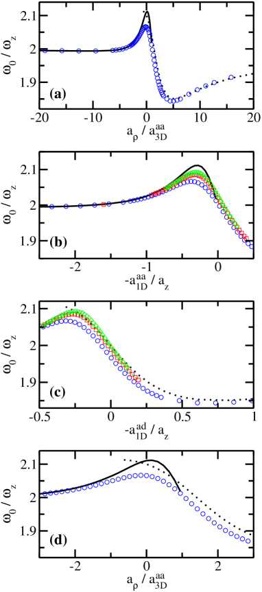
Figure 5: (Color online) Excitation frequency $\omega_{0}/\omega_{z}$ for $N=3$ with $P_{z}=+1$ and $r_{0}=0.01a_{z}$. (a) $\omega_{0}/\omega_{z}$ as a function of $a_{\rho}/a_{\mathrm{3D}}^{\mathrm{aa}}$ for $\lambda=10$. Circles show the 3D excitation frequency, while solid and dotted lines show the corresponding 1D quantities calculated using $H_{\mathrm{1D}}^{\mathrm{a}}$ and $H_{\mathrm{1D}}^{\mathrm{m}}$, respectively. Panels (b), (c) and (d) show the strongly-interacting regime in more detail. (b) $\omega_{0}/\omega_{z}$ as a function of $-a_{\mathrm{1D}}^{\mathrm{aa}}/a_{z}$. Circles, squares and diamonds show the 3D excitation frequency for $\lambda=10$, $15$ and 20. A solid line shows the corresponding 1D quantities calculated using $H_{\mathrm{1D}}^{\mathrm{a}}$. (c) $\omega_{0}/\omega_{z}$ as a function of $-a_{\mathrm{1D}}^{\mathrm{ad}}/a_{z}$. Circles, squares and diamonds show the 3D excitation frequency for $\lambda=10$, $15$ and 20. A dotted line shows the corresponding 1D quantities calculated using $H_{\mathrm{1D}}^{\mathrm{m}}$. (d) Enlargement of panel (a).

show the 3D excitation frequency $\omega_{0}$ for $N=3$ with $P_{z}=+1$ and $\lambda=10$. Panels (a) and (d) show $\omega_{0}$ as a function of $a_{\rho}/a_{\mathrm{3D}}^{\mathrm{aa}}$. The excitation frequency $\omega_{0}$ equals $2\omega_{z}$ in the NI limit ($a_{\mathrm{3D}}^{\mathrm{aa}}\rightarrow 0^{-}$), reaches its maximum for infinitely large $a_{\mathrm{3D}}^{\mathrm{aa}}$ and its minimum for $a_{\rho}/a_{\mathrm{3D}}^{\mathrm{aa}}\approx 5$, and increases monotonically towards $2\omega_{z}$ as $1/a_{\mathrm{3D}}^{\mathrm{aa}}$ increases further. To illustrate the dependence of $\omega_{0}$ on the aspect ratio, squares and diamonds in Figs. 5(b) and (c) show the 3D excitation frequency $\omega_{0}$ for two larger aspect ratios, i.e., for $\lambda=15$ and 20. Small dependencies of $\omega_{0}$ on $\lambda$ are visible in the strongly-interacting regime.

To ease comparisons between the 3D excitation frequencies and those based on the 1D Hamiltonian, Figs. 5(b) and (c) show enlargements of the strongly-interacting regime as functions of $-a_{\mathrm{1D}}^{\mathrm{aa}}/a_{z}$ and $-a_{\mathrm{1D}}^{\mathrm{ad}}/a_{z}$. These scales are chosen since $a_{\mathrm{1D}}^{\mathrm{aa}}$ and $a_{\mathrm{1D}}^{\mathrm{ad}}$ determine the properties of $H_{\mathrm{1D}}^{\mathrm{a}}$ and $H_{\mathrm{1D}}^{\mathrm{m}}$, respectively. Solid lines in Fig. 5 show the excitation frequencies calculated using the effective atomic 1D Hamiltonian. These 1D excitation frequencies reproduce the 3D excitation frequencies well in the weakly-attractive regime ($a_{\mathrm{1D}}^{\mathrm{aa}}$ large). In the strongly-interacting regime, the agreement improves with increasing $\lambda$ [see Fig. 5(b)]. Dotted lines in Fig. 5 show the 1D excitation frequencies calculated using $H_{\mathrm{1D}}^{\mathrm{m}}$. For large $|a_{\mathrm{1D}}^{\mathrm{ad}}|$ ($a_{\mathrm{1D}}^{\mathrm{ad}}<0$), the 3D excitation frequencies are independent of $\lambda$ and reproduced well by the 1D molecular model. For smaller $|a_{\mathrm{1D}}^{\mathrm{ad}}|$, the agreement improves with increasing $\lambda$ [see Fig. 5(c)].

The effective molecular 1D Hamiltonian $H_{\mathrm{1D}}^{\mathrm{m}}$ predicts that a subset of the $P_{z}=+1$ energy spectrum of the three- and four-particle systems coincides with that of a two-particle Tonks-Girardeau (TG) gas for $a_{\mathrm{1D}}^{\mathrm{ad}}=0$ olsh98 . For this atom-dimer scattering length, the effective molecular 1D Hamiltonian predicts $\Lambda_{2,1}=1$, $\Lambda_{2,2}=1/2$ and $\omega_{0}=2\omega_{z}$. Assuming that the behavior of the effective dimer system is indeed governed by $a_{\mathrm{1D}}^{\mathrm{ad}}$ (i.e., assuming that effective range and other corrections are negligible), the condition $a_{\mathrm{1D}}^{\mathrm{ad}}=0$ signals an atom-dimer resonance. Our 3D calculations for the three-particle system with $P_{z}=+1$ show that the ground state energy corresponds to that of a TG gas for $a_{\rho}/a_{\mathrm{3D}}^{\mathrm{aa}}\approx 1.54-1.58$ and that $\omega_{0}$ equals $2\omega_{z}$ for $a_{\rho}/a_{\mathrm{3D}}^{\mathrm{aa}}\approx 1.1-1.4$ for $\lambda=10-20$, in fairly good agreement with the prediction based on the 1D model, $a_{\rho}/a_{\mathrm{3D}}^{\mathrm{aa}}=1.4069$. The good agreement between our 3D results and those based on the effective molecular 1D Hamiltonian, which is based on a simple empirical parametrization of the effective 1D atom-dimer and dimer-dimer scattering lengths, suggests that the molecular 1D model employed in this work provides a viable and fairly accurate description of the system.

The atom-dimer $s$-wave resonance of quasi-1D systems found here, $a_{\rho}/a_{\mathrm{3D}}^{\mathrm{aa}}\approx 1.5$, is somewhat smaller than that found by Mora et al. moran3 by solving a set of integral equations for zero-range interactions, $a_{\rho}/a_{\mathrm{3D}}^{\mathrm{aa}}\approx 1.85$ footnoteelongatedcombine . The 3D Hamiltonian employed by Mora et al. accounts for the same physics as our 3D Hamiltonian and the determination of the effective 1D atom-dimer scattering length should, at least in principle, be exact moran3 . It is not clear at present why our empirical molecular 1D Hamiltonian provides a seemingly better description than Mora et al.’s results for $a_{\mathrm{1D}}^{\mathrm{ad}}\approx 0$.

We also analyzed the ground state energy and excitation spectrum for $N=4$. The four-particle 3D energies are harder to converge than the three-particle 3D energies, and comparisons between the full 3D excitation frequencies and the corresponding 1D quantities are accompanied by non-neglegible uncertainties. We find that our 3D results are consistent with the dimer-dimer $s$-wave resonance value predicted by $H_{\mathrm{1D}}^{\mathrm{m}}$ [Eq. (13) with $j=\mathrm{dd}$, and $a_{\mathrm{1D}}^{\mathrm{dd}}$ given by Eq. (11) with $\mathrm{aa}$ replaced by $\mathrm{dd}$], $a_{\rho}/a_{\mathrm{3D}}^{\mathrm{aa}}=0.89$ footnoteelongatedcombine .

V Conclusions

In summary, we have presented highly-accurate, microscopic 3D calculations for small highly-elongated Fermi gases with $N=2-4$ atoms and reported the energies as a function of the interaction strength, covering the weakly-attractive and weakly-repulsive regimes as well as the strongly-interacting regime. In addition, the dependence of the energies on the aspect ratio was investigated for selected cases. While the role of the aspect ratio is negligible in the weakly-interacting regimes, its role becomes more important in the strongly-interacting regime, possibly indicating that vitual excitations of transverse modes become relevant. The full 3D energy curves with $P_{z}=+1$ are reproduced to a good approximation by effective atomic and molecular 1D models whose effective interactions are given by simple analytical expressions that depend on the atom-atom $s$-wave scattering length $a_{\mathrm{3D}}^{\mathrm{aa}}$, the aspect ratio $\lambda$ and the atom mass $m$. We find that the energies obtained from these effective atomic and molecular 1D Hamiltonian join fairly smoothly in the strongly-interacting regime. Assuming that the effective 1D atom-dimer and dimer-dimer scattering lengths govern the behavior of the highly-elongated system, we deduced the positions of confinement-induced atom-dimer and dimer-dimer resonances from our energies. Whether the effective 1D models also connect fairly smoothly for larger systems is a pressing questions, in particular since the determination of the phase diagram of highly-elongated systems often times relies on strictly 1D treatments.

In the future, it will be interesting to extend the studies presented here to larger population-balanced and population-imbalanced two-component Fermi gases. While some microscopic calculations exist for strictly 1D systems, microscopic 3D treatments that accurately account for the dynamics along the tight and loose confining directions are challenging. Furthermore, it will be interesting to compare the 1D results obtained here for small systems with those obtained within the local density approximation and to extend analogous comparisons to larger systems.

Support by the NSF through grant PHY-0555316 is gratefully acknowledged.

References

- (1) S. Giorgini, L. P. Pitaevskii, and S. Stringari, Rev. Mod. Phys. 80, 1215 (2008). I. Bloch, J. Dalibard, and W. Zwerger, ibid. 80, 885 (2008).
- (2) News Focus, Science 320, 312 (2008).
- (3) E. H. Lieb and W. Liniger, Phys. Rev. 130, 1605 (1963). E. H. Lieb, ibid. 130, 1616 (1963). M. Gaudin, Phys. Lett. A 24, 55 (1967). C. N. Yang, Phys. Rev. Lett. 19, 1312 (1967).
- (4) M. Olshanii, Phys. Rev. Lett. 81, 938 (1998).
- (5) G. E. Astrakharchik, D. Blume, S. Giorgini, and B. E. Granger, Phys. Rev. Lett. 92, 030402 (2004); J. Phys. B 37, S205 (2004).
- (6) G. E. Astrakharchik, D. Blume, S. Giorgini, and L. P. Pitaevskii, Phys. Rev. Lett 93, 050402 (2004). G. Orso, ibid 98, 070402 (2007). H. Hu, X.-J. Liu, and P. D. Drummond, ibid. 98, 070403 (2007).
- (7) C. Mora, A. Komnik, R. Egger, and A. O. Gogolin, Phys. Rev. Lett. 95, 080403 (2005).
- (8) I. V. Tokatly, Phys. Rev. Lett. 93, 090405 (2004). J. N. Fuchs, A. Recati, and W. Zwerger, ibid. 93, 090408 (2004).
- (9) M. Köhl et al., Phys. Rev. Lett. 94, 080403 (2005). H. Moritz et al., ibid. 94, 210401 (2005).
- (10) Y. Suzuki and K. Varga, Stochastic Variational Approach to Quantum-Mechanical Few-Body Problems (Springer Verlag, Berlin, 1998).
- (11) H. H. B. Sørensen, D. V. Fedorov, and A. S. Jensen, Nuclei and Mesoscopic Physics, ed. by V. Zelevinsky, AIP Conf. Proc. No. 777 (AIP, Melville, NY, 2005), p. 12. J. von Stecher and C. H. Greene, Phys. Rev. Lett. 99, 090402 (2007).
- (12) J. von Stecher, C. H. Greene, and D. Blume, Phys. Rev. A 77, 043619 (2008).
- (13) J. von Stecher, C. H. Greene, and D. Blume, Phys. Rev. A 76, 053613 (2007).
- (14) T. Bergeman, M. G. Moore and M. Olshanii, Phys. Rev. Lett. 91, 163201 (2003).
- (15) D. S. Petrov, Phys. Rev. A 67, 010703(R) (2003).
- (16) D. S. Petrov, C. Salomon, and G. V. Shlyapnikov, Phys. Rev. Lett. 93, 090404 (2004).
- (17) C. Mora, R. Egger, A. O. Gogolin, and A. Komnik, Phys. Rev. Lett. 93, 170403 (2004). C. Mora, R. Egger, and A. O. Gogolin, Phys. Rev. A 71, 052705 (2005).
- (18) G. V. Skorniakov and K. A. Ter-Martirosian, Zh. Eksp. Teor. Fiz. 31, 775 (1956) [Sov. Phys. JETP 4, 648 (1957)].
- (19) T. Busch, B.-G. Englert, K. Rza̧żewski, and M. Wilkens, Foundations of Phys. 28, 549 (1998).
- (20) T. Cheon and T. Shigehara, Phys. Lett. A 243, 111 (1998); Phys. Rev. Lett. 82, 2536 (1999). M. D. Girardeau and H. Nguyen and M. Olshanii, Opt. Comm. 243, 3 (2004). K. Kanjilal and D. Blume, Phys. Rev. A 70, 042709 (2004).
- (21) Eq. (11) predicts an atom-dimer [dimer-dimer] resonance at [], which is smaller [larger] than [] moran3 ; mora05 .