Flow improvement caused by agents who ignore traffic rules

Abstract

A system of agents moving along a road in both directions is studied numerically within a cellular-automata formulation. An agent steps to the right with probability $q$ or to the left with $1-q$ when encountering other agents. Our model is restricted to two agent types, traffic-rule abiders ($q=1$) and traffic-rule ignorers ($q=1/2$). The traffic flow, resulting from the interaction between these two types of agents, is obtained as a function of density and relative fraction. The risk for jamming at a fixed density, when starting from a disordered situation, is smaller when every agent abides by a traffic rule than when all agents ignore the rule. Nevertheless, the absolute minimum occurs when a small fraction of ignorers are present within a majority of abiders. The characteristic features for the spatial structure of the flow pattern are obtained and discussed.

I Introduction

Society has various rules to regulate interactions among its members. While some of these rules might be enforced by authorities and turned into laws, quite a few have evolved over a long time and have turned into conventions. Just as in natural sciences, rules or conventions, regulating the interaction between individual constituents, often result in emerging global patterns. A traffic rule which enforces individual vehicles/pedestrians to move along only one side of a road clearly results in a global traffic flow pattern (see, e.g., Ref. young ). Because of this connection, traffic problems have often been studied by using methods and concepts from nonequilibrium statistical physics (for a review, see Refs. chow and helbing ). The approaches from physics include hydrodynamic descriptions hydro , differential equations describing effective microscopic forces ode , and cellular automata (CA) biham ; fukui ; mura ; automata ; lee2004a . In particular, the CA approach is often used in broad contexts of agent-based modeling as an efficient way of accounting for complicated interactions among constituents. Due to the computational efficiency, CA is particularly suitable for analyzing the dynamics of many individuals who try to move in different directions while at the same time being influenced by the motions of other individuals. It is notable that the jamming in vehicular traffics has natures different from that in pedestrian traffics. The former is explained by the time delay in the responses of the drivers, and this is the reason why the jamming may easily occur with vehicles only in one direction lee2004a . In the latter case, on the other hand, the jamming is caused by the collision of agents in opposite directions fukui . This study is mainly focused on this pedestrian case.

In the present work, we use the CA approach and find that the minimal risk for a jamming of the pedestrian flow occurs when a small fraction of traffic-rule ignorers is present within a majority of traffic-rule abiders. Even though this result is obtained within our simplified model system, it raises an interesting question on the observability and implication of such a phenomenon in social systems. Here we provide a detailed description on this observation as well as a qualitative understanding.

This paper is organized as follows. In Sec. II, we review the basics of a coordination game based on a traffic rule. We describe how we have performed our numerical experiments in Sec. III. The results are presented and compared to the coordination game in Sec. IV. The results are summarized in Sec. V.

II Coordination game

Let us first consider two players moving on a road in opposite directions heading for a direct collision. Each of them can choose to step aside left ($L$) or right ($R$) in order to avoid the collision and it is avoided only if both make the same choice. Thus the options both $L$ or both $R$ are equally gainful, whereas the choices $LR$ and $RL$ lead to collision. The situation is summarized in Table 1 in the form of a doubly-symmetric two-person coordination game davis ; weibull . Each player will behave according to a strategy in the form of a complete description of which action is taken under every possible circumstance. In what follows, we denote the strategy of an agent as $S_{q}$ if she chooses $R$ with probability $q$ (and thus $L$ with probability $1-q$). For example, if a player always chooses $R$ ($L$), her strategy is represented as $S_{1}$ ($S_{0}$).

Table 1: Normal form of a traffic-rule coordination game. Since the situation is symmetric to each player, only one player’s payoff is presented in this table after normalized to unity. Both players are better off when they choose the same moves (left/left and right/right).

	Left	Right
Left	1	0
Right	0	1

The concept of equilibrium is useful in analyzing a game: suppose that everyone has chosen a strategy so that no one gains anything by changing her strategy unilaterally, such a set of strategies constitute a Nash equilibrium weibull . In the case of the coordination game, there exist three strategies which are Nash equilibria, i.e., $S_{1}$, $S_{0}$, and $S_{1/2}$. The pure strategies $S_{1}$ and $S_{0}$ simply represent the ordinary traffic rules such that agents should always step aside to the right or always to the left. Due to the left-right symmetry in the problem both $S_{1}$ and $S_{0}$ compose Nash equilibria. On the other hand, if one makes a decision at random by tossing a coin, then obviously the opposing player cannot gain anything no matter what strategy she changes to. Consequently, the mixed strategy $S_{1/2}$ also constitutes a Nash equilibrium.

We next consider the evolutionary stabilities maynard of these Nash equilibria in a population where every pair of members plays the game. Suppose that almost all the players adopt a certain strategy $S$. The strategy $S$ is called evolutionarily stable when another mutant strategy $\tilde{S}$ cannot invade the population of $S$ since the payoff of $\tilde{S}$ is less than that of $S$. Mathematically, the evolutionary stability of the mixed strategy $S_{q}$ is equivalent to the stability of a population where a fraction $Q=q$ of members have $S_{1}$ while the others have $S_{0}$ maynard . Note that such equivalence holds only when there exist two pure strategies. In the stability analysis, one often employs a dynamics resulting as individuals in a group try to adopt the strategies of more successful individuals. Such a situation can be modeled as follows: the relative proportion $Q_{S}$ of players who use strategy $S$ is assumed to grow in time in proportion to the payoff $W_{S}$ at the last time step. This particular dynamics is given by the replicator dynamics equations maynard ,

$$\dot{Q_{S}}\equiv\frac{dQ_{S}}{dt}=Q_{S}\left(W_{S}-\sum_{S^{\prime}}W_{S^{\prime}}Q_{S^{\prime}}\right)$$

within the continuum time approximation, where the last term has been inserted to make the constraint $\sum_{S}Q_{S}=1$ fulfilled at any time $t$. In our traffic-rule game, we have $Q_{S_{0}}+Q_{S_{1}}=1$, and therefore we may set $Q_{S_{1}}\equiv Q$ and $Q_{S_{0}}\equiv 1-Q$ to study the evolutionary stability of $S_{q}$ with $q=Q$. From Table 1, it follows that the expected pay-off for an agent is given by the probability of encountering a traffic-rule abider or ignorer, respectively, resulting in $W_{S_{1}}=Q$ and $W_{S_{0}}=1-Q$. For example, if $Q=1/4$, an agent with strategy $S_{1}$ will have a chance out of four to meet another with the same strategy, meaning that her expected payoff amounts to $1/4$ at every encounter. Consequently, the replicator dynamics equations can be cast in the form

$$\dot{Q} = Q\{Q-[Q^{2}+(1-Q)^{2}]\}$$

$$= Q(1-Q)(2Q-1).$$

From the stationarity condition $\dot{Q}=0$ we find three Nash equilibria at $Q_{1}=0$, $Q_{2}=1$, and $Q_{3}=1/2$, which in turn correspond to $q=0,1$, and $1/2$, respectively. The linear perturbation $\epsilon_{n}$ introduced to the $n$th Nash equilibrium by $Q=Q_{n}+\epsilon_{n}$ ($n=1,2,3$) satisfies $\dot{\epsilon_{1}}/\epsilon_{1}<0$, $\dot{\epsilon_{2}}/\epsilon_{2}<0$, and $\dot{\epsilon_{3}}/\epsilon_{3}>0$, respectively, and we find that only the last equilibrium point $Q=1/2$ is unstable in this dynamics. In other words, a convention of randomly choosing left or right is unlikely to emerge, since people eventually learn that the traffic improves if a majority settles for one of the alternatives. Note that this conclusion is based on the assumption of full mixing, corresponding to the mean-field approximation in physics. To what extent is the simple picture, implied by Table 1, also valid for a two-dimensional plane filled with moving agents? This question is investigated in the following.

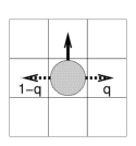
Figure 1: Movements of a self-propelled agent. The solid arrow indicates the agent’s intrinsic direction, while the dotted ones indicate its possible evasions when the intrinsic direction is blocked by another agent.

III Numerical setup

III.1 Moving code

We start with a simple self-propelled agent, derived from Ref. mura , which obeys the following moving code (compare to Fig. 1). It has its own intrinsic direction, either upward or downward. It can move only to a neighboring cell at each time step, and a single cell cannot allow more than one agent at the same time. If the agent’s front cell is empty, it moves to the cell with the probability $1-s$, where $s$ denotes the probability of spontaneous stopping. If the agent is prevented from moving forward, because the front cell is already occupied, then it steps aside to the right with a probability $q$ or to the left with $1-q$. In case it attempts to the right (left) but cannot because there is already an agent in that cell, then it proceeds to try the alternative option left (right). In case this is also prevented, it just remains in its present cell. At least two steady states can be found within this moving code: one is the complete jamming where no one can move forward and the other one is a perfectly collisionless flow where every column is occupied only by agents moving in the same direction.

III.2 Initialization

A road is a two-dimensional plane, which has a size of $X\times Y$ in units of cells. We impose a periodic boundary (PB) in the $y$ direction to make the road homogeneous in that direction. In the $x$ direction, on the other hand, there are walls which prevent agents from being at $x\leq 0$ or $x>X$. At the initial time, the agents are randomly distributed with a density $\rho$ on the road, and their intrinsic directions are given upward or downward with equal probability. Such a starting condition is qualitatively similar to a walking street filled with mingled pedestrians which all start to walk home at the same moment. The number of agents is $N=\rho XY$, and the numbers of upward and downward agents are $N/2$. Among these $N$ agents, $pN$ agents have $q=1$ so that they always try the right-hand side first, while the others have no preferences, i.e., $q=1/2$. There are no initial correlations among the position, intrinsic direction, and preference.

III.3 Recursive update

All agents make moves in accordance with the moving code in a random sequential order (RSO). A simultaneous update is, in practice, not possible since each update then involves finding all consistent possibilities based on all individual possibilities of all the agents. The RSO update together with the PB condition causes an artifact called deadlock. Imagine that one column is fully occupied by players having the same intrinsic direction with zero stopping probability ($s=0$). Even though all of them want to move in the same direction, they cannot within the RSO update since no one finds an empty space in front of herself. Therefore, RSO needs to be modified as follows. Suppose that an agent $A$ is picked up by RSO to be updated. Then we regard $A$’s current position as empty and search for a new position for it according to the moving code. If agent $A$ is blocked from going forward by another agent $B$, which has the same intrinsic direction as $A$ but not updated yet at this time step, we do not exclude the possibility for both of them to move together simultaneously, so we let $B$ move first. If $B$ is also in the same situation by a third agent $C$, this procedure is repeated recursively. When this recursion goes all the way around PB to $A$’s position again, the column of agents will be updated by one cell forward altogether. One time step is completed when the moving code is applied to all the $N$ agents.

IV Results

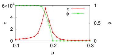
Figure 2: (Color online) Transition between two steady states, the complete jamming and the collisionless flow, as density $\rho$ changes. Both of the fraction $p$ of rule abiders and the stopping probability $s$ are set to zero and the road is given as $50\times 200$. Depicted here are the flow $\phi$ and the time $\tau$ to either of the steady states after being averaged over $10^{3}$ samples under a cutoff of $t_{c}=10^{6}$.

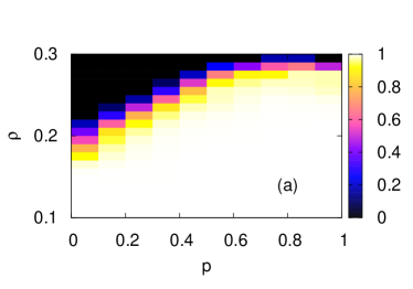
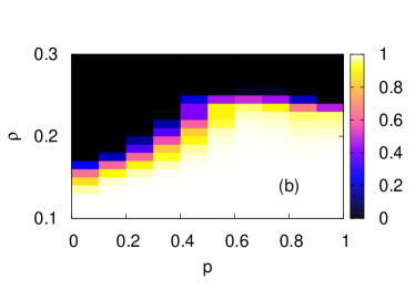
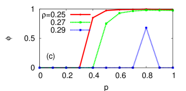
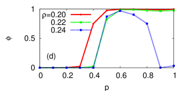
Figure 3: (Color online) Flow $\phi$, as a function of $\rho$ and $p$, with the stopping probability $s=0$. The road sizes are (a) $50\times 200$ and (b) $100\times 400$, respectively. Each point is obtained from $10^{3}$ random initial conditions. Completely black region indicates that the system is in a traffic jam, one of the steady states, while all the agents move freely when the parameters $p$ and $\rho$ are within the white region corresponding to $\phi=1$. $10^{3}$ samples. (c) Sectional plots of $\phi$ with fixing $\rho$ in $50\times 200$ and (d) in $100\times 400$. The nonmonotonic behavior of $\phi$ is more pronounced in the latter case, which has enough room for developing spatial patterns as described in the text.

A crucial question, when it comes to traffic flow, is under what conditions the traffic will jam. This usually happens when the traffic gets too dense. Hence, one may expect that there exists a critical traffic density $\rho=\rho_{c}$ beyond which the propensity for jamming becomes high. In our traffic model we measure the traffic flow $\phi$, the fraction of agents advancing in its intrinsic direction, at a given density of agents $\rho$ and average over a large number of random initializations. Figure 2 shows one example, together with the average time $\tau$ taken to reach a steady situation, which is either a jam or a steady-state flow. Close to $\rho_{c}$ the time to reach a steady situation becomes so large that we, for practical reasons, introduce a large time cut-off $t_{c}$ in the simulations. As illustrated in Fig. 2, there is a sharp cross over from a low- to a high-risk jamming at around a well-defined critical density $\rho_{c}$. The flow $\phi$ is averaged over $10^{3}$ samples in this figure and determined by how many samples will settle down to the steady flow. Intuitively one would expect that $\rho_{c}$ decreases as we make the road larger for a fixed density of agents and fixed width of the road; any point along the road is a potential site where a jamming could start and grow into a road block across the road which implies that the longer the road the larger the risk for jamming (see, for comparison, Ref. biham ). In Fig. 3 it is shown that this is also true in the case where the width and the length increase simultaneously, preserving the geometrical shape of the road. Since $\rho_{c}$ decreases as the size of the road increases (even when the geometrical shape is preserved), we speculate that the jamming transition has the large-size limit $\rho_{c}=0$ in our model. This also implies that the capacity of a road, measured as the amount of traffic that a road will transmit on average before the traffic jams, increases less than linearly with the road size.

A striking feature of Fig. 3 is that $\rho_{c}$ does not grow monotonically with the proportion of traffic-rule abiders $p$. In other words, when only $60\%$ of agents abide by the rule, for example, the road of $100\times 400$ has a higher capacity than when $90\%$ abide by the rule.

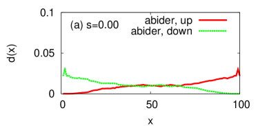
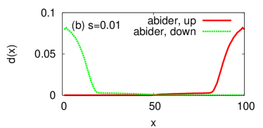
Figure 4: (Color online) Snapshots of density distributions in the long run when only rule abiders are present ($p=1$). The average is taken over about $10^{3}$ samples at $t\geq 6\times 10^{4}$, where $X=100$, $Y=400$, and $\rho=0.2$. The stopping probability is set as (a) $s=0$ and (b) $s=0.01$, respectively.

One possible guess would be that the traffic reduction with abundant rule abiders is caused by their concentration on the wall sides, since it is an inefficient use of resources if they are populated only at those parts of the road. However, that scenario does not explain this phenomenon. Let us plot the spatial density $d(x)$ for the groups of pedestrians so that $\sum_{x}d(x)=1$ is satisfied for each group. Rule abiders do not occupy only the sides of the road if the stopping probability $s$ is zero because then rule abiders have no reason to move in the lateral direction once forming a lane anywhere on the road [Fig. 4(a)]. Even if $s\neq 0$ as in Fig. 4(b), a high density of agents does not disturb the maximal flow velocity due to the recursive update (Sec. III.3).

In order to gain some further insight into the mutual effect between rule abiders and rule ignorers, we have studied the spatial flow structure in more detail. To this end it is convenient to include a tiny nonzero stopping probability $s$ (we use $s=0.01$ in the simulations) for the following reason: whenever an agent stops, agents colliding from behind try to step aside as prescribed by the moving code. Hence a nonzero stopping probability generates small diffusive processes in the lateral direction. This helps the system to arrive at a robust spatial steady state without changing the numerical results in any essential way.

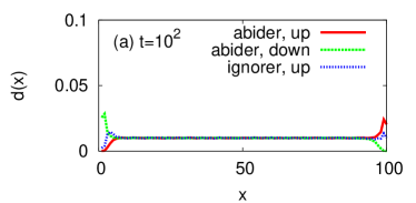
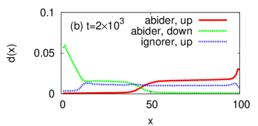
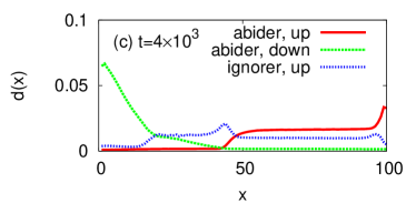
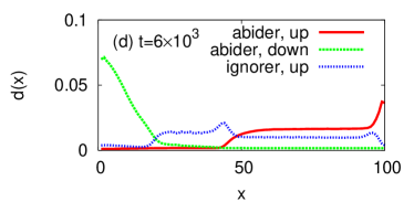
Figure 5: (Color online) Snapshots of density distributions with the condition that rule ignorers move only upward. The average is taken over $10^{3}$ samples, where $X=100$, $Y=400$, $\rho=0.2$, $p=0.9$, and $s=0.01$. (a) $t=10^{2}$, (b) $t=2\times 10^{3}$, (c) $t=4\times 10^{3}$, and (d) $t=6\times 10^{3}$.

For simplicity we choose the case when the rule ignorers are restricted to move upward (Fig. 5). According to the moving code, agents moving in opposite directions will have a stronger interaction than agents moving in the same direction. Since rule abiders always prefer the right-hand side, the most rapid process is the pushing of the downward rule abiders to the left side of the plot in order to avoid agents moving upward [Fig. 5(b)]. By symmetry the upward rule abiders get pushed out of the left region preferred by the downward rule abiders. However, rule ignorers have no preference between left and right, and as a consequence they remain for a longer time in the middle region. Their presence further pushes the downward rule abiders to the left wall. Note that the upward rule abiders, on the other hand, have little interaction with rule ignorers since all of them are basically headed for the same direction. As these upward rule abiders move very slowly in the $x$ direction, many of the rule ignorers cannot penetrate into the right side, i.e., $x>50$, but remain on the wrong side of the road with respect to the traffic rule [Fig. 5(d)].

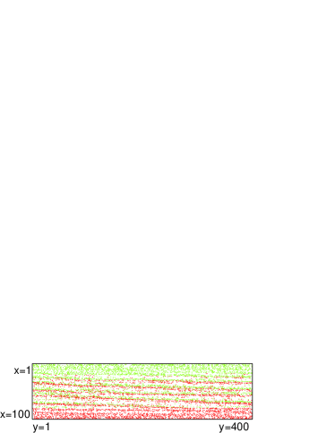
Figure 6: (Color online) A typical distribution of agents taken from a sample at $t=10^{3}$ with $\rho=0.2$, $p=1.0$, and $s=0.01$, where the road is given as $100\times 400$. Two intrinsic directions are marked with different colors so that red (dark) dots mean upward rule abiders and green (bright) dots mean downward rule abiders.

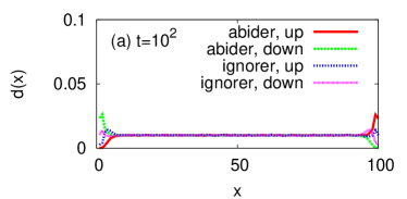
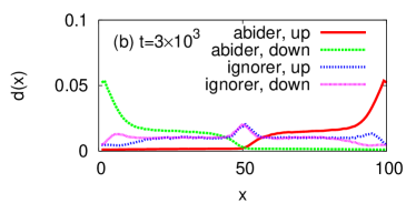
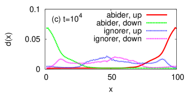
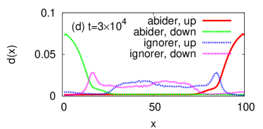
Figure 7: (Color online) Snapshots of density distributions, when both of upward and downward rule ignorers are present. The average is taken over $10^{3}$ samples, where $X=100$, $Y=400$, $\rho=0.2$, $p=0.9$, and $s=0.01$. (a) $t=10^{2}$, (b) $t=3\times 10^{3}$, (c) $t=10^{4}$, and (d) $t=3\times 10^{4}$.

Also in the case which includes downward rule ignorers in addition, rule abiders are more quickly evacuated from the central part of the road in the presence of rule ignorers. In addition, rule ignorers play an important role in smoothing out uneven agent concentrations on the road. These uneven concentrations arise because the upward rule abiders have an average drift toward the right side of Fig. 5, when starting from a random initial condition, while downward rule abiders drift in the opposite direction. As a consequence they interact and usually form long narrow trains in the central part of the road (Fig. 6). This leads to high local concentrations on the road from which jamming can start and develop. However, with a sufficient number of rule ignorers, these trains are broken into a more evenly distributed concentration, reducing the risk of jamming.

Snapshots of the flow development for the case including downward rule ignorers as well as upward rule ignorers are shown in Fig. 7. One notable point is that the rule ignorers tend to make a backflow against the rule abiders. One sees abundance of upward rule ignorers on the left-hand side of the median line at $x=X/2$ and conversely abundance of downward rule ignorers on the right-hand side of the median line [Fig. 7(d)]. The upward (downward) backflow is developed by rule ignorers who are repelled by downward (upward) movers gathering densely beside the left (right) wall. This is a numerically stable pattern which is rather unexpected from an intuitive point of view.

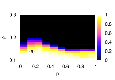
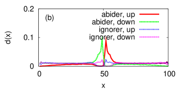
Figure 8: (Color online) (a) Flow $\phi$, as a function of $\rho$ and $p$, when the traffic rule is applied only to rule abiders on the wrong side of the road. In accordance to Fig. 3, we take averages over $10^{3}$ samples with a size of $100\times 400$ and set $s=0$. (b) A snapshot of the spatial distribution for $\rho=0.1$ and $p=0.9$, taken at $t=6\times 10^{4}$. This shape maintains itself with time for $s=0$, while for a nonzero $s$, the peaks on the middle are slowly relaxed outward.

Finally, we have tested how much the result changes with a variation in the moving code. The traffic rule becomes softened so that it acts only to rule abiders on the wrong side of the road. If standing on the right side, even rule abiders will be just the same as rule ignorers. This rule was designed to check whether the excessive concentration on the wall sides, as in Fig. 4(b), could be relaxed without altering the qualitative results. Numerical simulations show that the nonmonotonic behavior of $\rho$ still remains and the optimal $p$ is even lowered than before [Fig. 8(a)]. A closer look indicates that jamming is likely to develop around the median line $x=X/2$, since the momentum of rule abiders to the right side disappears while crossing the line, leading to congestion at that point [Fig. 8(b)].

V Summary

In our numerical simulation based on the CA approach, we have observed that the jamming transition density on two-dimensional planes does not monotonically increase with the fraction of rule abiders. It implies that a certain amount of rule ignorers may diminish the propensity for jamming by diminishing the risk for high local traffic concentrations. In contrast to the coordination game, which presumes two rational players acting to maximize the gain by either abiding to or breaking the traffic rule, the situation on a large road is generally more complex; it involves interactions among agents which lead to nontrivial flow patterns in a long time. Our result suggests that there are situations when abiding too strictly by a traffic rule could lead to a jamming disaster which would be avoided if some people just ignored the traffic rule altogether.

One should note that this is drawn by our model system under certain conditions, which captures only a part of the pedestrian dynamics. Our observation demonstrates one possible complexity of the pedestrian problem that even such simple agents could lead to an unexpected global behavior. It also supports to some extent a hypothesis that the most successful behavior in social or biological systems is achieved when both of the regular and random factors are incorporated, which should be further examined in future research.

- (1) H. P. Young, Individual Strategy and Social Structure (Princeton University Press, Princeton, NJ, 1998).
- (2) D. Chowdhury, L. Santen, and A. Schadschneider, Phys. Rep. 329, 199 (2000).
- (3) D. Helbing, Rev. Mod. Phys. 73, 1067 (2001).
- (4) M. J. Lighthill and G. B. Whitham, Proc. R. Soc. London, Ser. A 229, 281 (1955); B. S. Kerner and P. Konhäuser, Phys. Rev. E 48, R2335 (1993); H. Y. Lee, H.-W. Lee, and D. Kim, Phys. Rev. Lett. 81, 1130 (1998).
- (5) L. A. Pipes, J. Appl. Phys. 24, 274 (1953); M. Bando, K. Hasebe, A. Nakayama, A. Shibata, and Y. Sugiyama, Phys. Rev. E 51, 1035 (1995); H. K. Lee, H.-W. Lee, and D. Kim, Phys. Rev. E 64, 056126 (2001); D. Helbing and P. Molnár, Phys. Rev. E 51, 4282 (1995).
- (6) O. Biham, A. A. Middleton, and D. Levine, Phys. Rev. A 46, R6124 (1992).
- (7) M. Fukui and Y. Ishibashi, J. Phys. Soc. Jpn. 68, 3738 (1999).
- (8) M. Muramatsu, T. Irie, and T. Nagatani, Physica A 267, 487 (1999).
- (9) K. Takimoto, Y. Tajima, and T. Nagatani, Physica A 308, 460 (2002); G. M. Hodgson and T. Knudsen, J. Econ. Behav. & Organ. 54, 19 (2004); W. G. Weng, T. Chen, H. Y. Yuan, and W. C. Fan, Phys. Rev. E 74, 036102 (2006); Y. F. Yu and W. G. Song, Phys. Rev. E 76, 026102 (2007).
- (10) H. K. Lee, R. Barlovic, M. Schreckenberg, and D. Kim, Phys. Rev. Lett. 92, 238702 (2004).
- (11) M. D. Davis, Game Theory: A Nontechnical Introduction (Basic, New York, 1970).
- (12) J. W. Weibull, Evolutionary Game Theory (MIT, Cambridge, MA, 1995).
- (13) J. M. Smith, Evolution and the Theory of Games (Cambridge University Press, Cambridge, England, 1982).