Physical Reference Frames and Astrometric Measurements of Star Direction in General Relativity
I. Stellar Aberration

Abstract

The high accuracy of modern space astrometry requires the use of General Relativity to model the propagation of stellar light through the gravitational field encountered from a source to a given observer inside the Solar System. In this sense relativistic astrometry is part of fundamental physics. The general relativistic definition of astrometric measurement needs an appropriate use of the concept of reference frame, which should then be linked to the conventions of the IAU Resolutions (IAU, 2000), which fix the celestial coordinate system. A consistent definition of the astrometric observables in the context of General Relativity is also essential to find uniquely the stellar coordinates and proper motion, this being the main physical task of the inverse ray tracing problem. Aim of this work is to set the level of reciprocal consistency of two relativistic models, GREM and RAMOD (Gaia, ESA mission), in order to garantee a physically correct definition of light direction to a star, an essential item for deducing the star coordinates and proper motion within the same level of measurement accuracy.

I introduction

The correct definition of a physical measurement requires the identification of an appropriate frame of reference. This applies also to the case of the determination of position and motion of a star from astrometric observations made from within our Solar System. Moreover, modern instruments homed into space-borne astrometric probes like Gaia (Turon et al., 2005) and SIM (Unwin et al., 2008) are targeting accuracy at the micro-arsecond level, or higher, thus requiring any astrometric measurement be modelled in a way that light propagation and detection are both conceived in a general relativistic framework. One needs, in fact, to solve the relativistic equations of the null geodesic which describes the trajectory of a photon emitted by a star and detected by an observer with an assigned state of motion. The whole process takes place in a geometrical environment generated by an N-body distribution as could be that of our Solar System. Essential to the solution of the above astrometric problem, namely an inverse ray tracing from observational data, is the identification, as boundary conditions, of the local observer’s line-of-sight defined in a suitable reference frame (see, e.g. (Bini et al., 2003; de Felice et al., 2006; de Felice and Preti, 2006)).

Summarizing from the references quoted above, the astrometric problem consists in the determination, from a prescribed set of observational data (hereafter observables) of the astrometric parameters of a star namely its coordinates, parallax, and proper motion. However, while in classical (non relativistic) astrometry these quantities are well defined, in General Relativity (GR) they must be interpreted consistently with the relativistic framework of the model. Similarly, the parameters describing the attitude and the center-of-mass motion of the satellite need to be defined consistently with the chosen relativistic model.

At present, three conceptual frameworks are able to treat the astrometric problem at the micro-arcsecond level within a relativistic context.

The first model, named GREM (Gaia Relativsitic Model) and described in Klioner (2003), is an extension of a seminal study Klioner and Kopeikin (1992) conducted in the framework of the post-Newtonian (pN) approximation of GR. This model has been formulated according to a Parametrized Post Newtonian (PPN) scheme accurate to 1 micro-arcsecond. In this model finite dimensions and angular momentum of the bodies of the Solar System are included and linked to the motion of the observer in order to consider the effects of parallax, aberration, and proper motion. This model is considered as baseline for the Gaia data reduction (Lattanzi et al., 2006). The boundary conditions are fixed by the coordinate position of the satellite and imposing the value of $c$ to the modulus of the light direction at past null infinity. The light path is solved using a matching technique which links the perturbed internal solution inside the near-zone of the Solar System with the (assumed) flat external one.

Conceptually similar to the above model is the one developed in Kopeikin and Schäfer (1999). Using the post-Minkowskian (pM) approximation, Einstein’s equations are solved in the linear regime expressing the perturbated part of the metric tensor in terms of retarded Lienard-Weichert potentials. Later, Kopeikin and Mashhoon (2002) included all the relativistic effects related to the gravitomagnetic field produced by the traslational velocity/spin-depedent metric terms.

Both works, in the pN and pM aproaches, rewrite the null geodesic as function of two independent parameters and solve the light trajectory as a straight line (Euclidean geometry) plus integrals, containing the perturbations encountered, from a gravitating source at an arbitrary distance from an observer located within the Solar System. This allows one to transform the observed light ray in a suitable coordinate direction and to read-off the aberrational terms and light deflections effects, evaluated at the point of observation. The main difference between the two approximations appears in the computation of the light deflection contributions: in the pN scheme by the technique of asymptotic matching, while in the pM one by a semi-analytical integration of the equation of light propagation from the observer to the source with retarted time as argument.

The third and last model, RAMOD, is an astrometric model conceived to solve the inverse ray-tracing problem in a general relativistic framework not constrained by a priori approximations (de Felice et al., 2004, 2006). It exploits the concept of a curved geometry as a common background to all steps of its functioning and can be extended to whatever accuracy and physical requirements (de Felice and Clarke, 1990). RAMOD therefore is not a just a pN model, contrary to how was referenced in (Teyssandier and Le Poncin-Lafitte, 2006). Moreover, the same parametrization of the pN/pM approximations can be obtained in RAMOD if we limit the model accuracy to the milli-arcsecond level (Crosta, 2003). The full development to the micro-arcsecond level imposes to include the $h_{0i}$ metric terms and to take properly into account the retarded distance effects due to the motion of the bodies of the Solar System (de Felice et al., 2006). At present, the RAMOD full solution requires the numerical integration of a set of coupled non linear differential equations (also called “master equations”) which allows to trace back the light trajectory to the star initial position and which naturally includes all the effects due to the curvature of the background geometry. A solution of this system of differential equations contains all the relativistic perturbations suffered by the photon along its trajectories due to the intervening gravitational fields. The boundary conditions fixed by the astrometric observable as function of an analytical fully relativistic description of the satellite allows a unique solution for a stellar position and motion (Bini et al., 2003).

The first two models, namely the pN and pM ones, though different, take advantage of a similar “language” that facilitate their comparison. RAMOD, on the contrary, is formulated in a completely different way. This makes its comparison with the former two a difficult task. However, since they are used for the Gaia data reduction with the purpose to create a catalog of absolute positions and proper motions, any inconsistency in the relativistic model(s) would invalidate the quality and reliability of the estimates. This alone is sufficient reason for making a theoretical comparison of the two approaches a necessity.

In this paper we present the first theoretical comparison, showing how it is possible to “extract” the aberration terms from the RAMOD construct.

In section II we review all the building steps of the RAMOD astrometric set-up. In section III we compare the procedures used in GREM to those utilized in RAMOD to define the observables and suggest a possible way to make a comparison between the quantities of these two formulations via the explicitation of the aberration part in the RAMOD framework. Section IV is devoted to describe the GREM calculations of stellar aberration, while the following one shows how the same effect can be recovered in RAMOD. Section VI will finally comment on the results of the comparison and on some crucial points which have to be addressed to proceed further with the theoretical comparison of the two models.

II The RAMOD frames

The set-up of any astrometric model implies, primarly, the identification of the gravitational sources and of the background geometry. Then one needs to label the space-time points with a coordinate system. The above steps allow us to fix a reference frame with respect to which one describes the light trajectory, the motion of the stars and that of the observer.

The RAMOD framework is based on the weak-field requirement for the background geometry, which in turn has to be specialized to the particular case one wants to model. For example, having in mind a Gaia-like mission, we can assume the Solar System as the only source of gravity, i.e. a physical system gravitationally bound and weakly relativistic. Then, only first order terms in the metric perturbation $h$ (or equivalently in the constant $G$ as in the post-Minkowskian approximation) are retained. These terms already include all of the possible $(v/c)^{n}$-order expansions of post-Newtonian approach, but just those up to $(v/c)^{3}$ are needed to reach the micro-arcsecond accuracy required for the next generation astrometric missions, like e.g. Gaia and SIM.

With these assumptions the background geometry is given by the following line element

$$\mathrm{d}s^{2}\equiv g_{\alpha\beta}\mathrm{d}x^{\alpha}\mathrm{d}x^{\beta}=\left(\eta_{\alpha\beta}+h_{\alpha\beta}+\mathcal{O}\left(h^{2}\right)\right)\mathrm{d}x^{\alpha}\mathrm{d}x^{\beta},$$

where $\mathcal{O}(h^{2})$ collects all non linear terms in $h$, the coordinates are $x^{0}=t,x^{1}=x,x^{2}=y,x^{3}=z$, the origin being fixed at the barycenter of the Solar System, and $\eta_{\alpha\beta}$ is the Minkowskian metric.

For this reason, any comparison between RAMOD and GREM requires that both use the same metric. In the small curvature limit the metric components used in RAMOD are (Misner et al., 1973)

$$g_{00}=-1+\underset{(2)}{h_{00}}+\mathcal{O}\left(4\right)\qquad g_{0i}=\underset{(3)}{h_{0i}}+\mathcal{O}\left(5\right)\qquad g_{ij}=1+\underset{(2)}{h_{00}}\delta_{ij}+\mathcal{O}\left(4\right),$$ (1)

where $\underset{(2)}{h_{00}}=2U/c^{2}$, $\underset{(3)}{h_{0i}}=U^{i}/c^{3}$, and $U$ and $U^{i}$ are, respectively, the gravitational potential and the vector potential generated by all the sources inside the Solar System that can be chosen according the IAU resolution B1.3 (IAU, 2000). The metric of Eq. (1) is also adopted by GREM. Finally the subscripts indicate the order of $(v/c)$ (e.g. $\underset{(3)}{h_{0i}}\sim\mathcal{O}(3)$ and $\mathcal{O}(n)=\mathcal{O}[(v/c)^{n}]$).

II.1 The BCRS

In the near zone of the Solar System and with the metric (1), IAU resolutions provide the definition of the Barycentric Celestial Reference System (BCRS), and of the Satellite Reference System (SRS) (IAU, 2000). These resolutions, as remarked above, are based on the pN approximation of GR which is still consistent with RAMOD, since the perturbation $h_{\alpha\beta}$ to the Minkowskian metric in (1) can be calculated at any desired order of approximations in $\left(v/c\right)$ inside the Solar System.

In RAMOD (see de Felice et al. (2004)) a BCRS is identified requiring that a smooth family of space-like hypersurfaces exists with equation $t\left(x,y,z\right)=\mathrm{const}$. The function $t$ can be taken as a time coordinate. On each of these $t\left(x,y,z\right)=\mathrm{const}$ hypersurfaces one can choose a set of Cartesian-like coordinates centered at the barycenter of the Solar System (B) and running smoothly as parameters along curves which point to distant cosmic sources. The latters are chosen to assure that the system is kinematically non-rotating. The parameters $x$, $y$, $z$, together with the time coordinate $t$, provides a basic coordinate representation of the space-time.

Any tensorial quantity will be expressed in terms of coordinate components relative to coordinate bases induced by the BCRS.

II.2 The local BCRS

In RAMOD, at any space-time point there exists a unitary four-vector $u^{\alpha}$ which is tangent to the world line of a physical observer at rest with respect to the spatial grid of the BCRS defined as:

$$u^{\alpha}=\left(-g_{00}\right)^{-1/2}\delta_{0}^{\alpha}=\left(1+\frac{U}{c^{2}}\right)\mathbf{\partial}_{t}+\mathcal{O}\left(\frac{v^{4}}{c^{4}}\right).$$ (2)

The totality of these four-vectors over the space-time forms a vector field which is proportional to a time-like and asymptotically Killing vector field (de Felice et al., 2004). The proper time measured by each of these observers is proportional to the BCRS coordinate time according to equation (2). To the order of accuracy required for Gaia, the rest space of $\mathbf{u}$ can be locally identified by a spatial triad of unitary and orthogonal vectors whose choice however can only be dictated by specific requirements. A natural choice is that of pointing to the local coordinate directions chosen of the BCRS (figure 1).

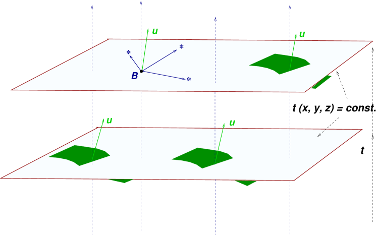
Figure 1: The local observer world line with respect to the BCRS coordinate system. The spatial axes of the BCRS point toward distant sources. The dashed lines are the world lines of the observers at rest with respect to the barycenter (B). The rest-space (green area) of $\mathbf{u}$ locally deviates from the space-like hypersurface with equation $t(x,y,z)=\mathrm{const}$ by terms of the order of a micro-arcsecond.

This frame will be called local BCRS; obviously, the local proper time varies as a function of the gravitational potential at the observer’s position, as can be deduced from equation (2). In the RAMOD formalism this local BCRS is represented by a tetrad whose spatial axes (the triad) coincide with the local coordinate axes, but whose origin is the barycenter of the satellite. At the $\mathcal{O}\left(h^{2}\right)$, this triad is (Bini et al., 2003)

$$\lambda_{\hat{a}}^{\alpha} = h_{0a}\delta_{0}^{\alpha}+\left(1-\frac{h_{00}}{2}\right)\delta_{a}^{\alpha}$$ (3)

for $a=1,2,3$.

In RAMOD any physical measurement refers to the local BCRS.

II.3 The proper reference frame for the satellite

The proper reference frame of a satellite consists of its rest-space and a clock which measures the satellite proper time.

The tensorial quantity which expresses a proper reference frame of a given observer is a tetrad adapted to that observer, namely a set of four unitary mutually orthogonal four-vectors $\mathbf{\mathbf{\lambda}_{\hat{\alpha}}}$ one of which, i.e. $\mathbf{\lambda}_{\hat{0}}$, is the observer’s four-velocity while the other $\mathbf{\lambda}_{\hat{a}}$s form a spatial triad of space-like four-vectors. Mathematically the tetrad is found as a solution of the following system (Misner et al., 1973):

$$\eta_{ab}=g_{\mu\nu}\lambda_{\hat{a}}^{\mu}\lambda_{\hat{b}}^{\nu}$$ (4)

which allows one to interpret a tetrad frame also as an instantaneous inertial reference frame. The solution of (4), always computed w.r.t. the BCRS, is not trivial since it depends on the metric at each space-time point along the world line of the observer. The physical measurements made by the observer (satellite) represented by such a tetrad are obtained by projecting the appropriate tensorial quantities on the tetrad axes.

The same measurements can also be defined by splitting the space-time into two subspaces. A time-like observer $u^{\prime\alpha}$ carrying its laboratory is usually represented as a world tube; in the case of a non-extended body, the world tube can be restricted to a world line tracing the history of the observer’s barycenter in the given space-time. At any point $P$ along the world line of $u^{\prime\alpha}$, and within a sufficiently small neighborhood, it is possible to split the space-time into a one-dimensional space and a three-dimensional one (de Felice and Clarke, 1990), each space being endowed with its own metric, respectively $U_{\alpha\beta}\left(u^{\prime}\right)=-u^{\prime}_{\alpha}u^{\prime}_{\beta}$ and $P_{\alpha\beta}\left(u^{\prime}\right)=g_{\alpha\beta}+u^{\prime}_{\alpha}u^{\prime}_{\beta}$. Clearly,

$$g_{\alpha\beta}=U_{\alpha\beta}\left(u^{\prime}\right)+P_{\alpha\beta}\left(u^{\prime}\right).$$ (5)

The space with metric $P_{\alpha\beta}\left(u^{\prime}\right)$ is generated by lines which stem orthogonally to the world-line of $\mathbf{u^{\prime}}$ at $P$ and is denoted as the rest-space of the observer $\mathbf{u^{\prime}}$ at $P$. In this space one measures proper lengths. The space with metric $U_{\alpha\beta}\left(u^{\prime}\right)$ is generated by lines which differ from that of $\mathbf{u^{\prime}}$ by a riparametrization. In this space one measures the observer’s proper time.

As a consequence of Equation (5), the invariant interval between two events in space-time can be written as $\mathrm{d}s^{2}=P_{\alpha\beta}\left(u^{\prime}\right)\,\mathrm{d}x^{\alpha}\mathrm{d}x^{\beta}+U_{\alpha\beta}\left(u^{\prime}\right)\,\mathrm{d}x^{\alpha}\mathrm{d}x^{\beta}$, from which we are able to extract the measurements of infinitesimal spatial distances and times intervals taken by ${\bf u}^{\prime}$ as, respectively, $\mathrm{d}L_{u^{\prime}}=\sqrt{P_{\alpha\beta}\left(u^{\prime}\right)\mathrm{d}x^{\alpha}\mathrm{d}x^{\beta}}$ and

$$\mathrm{d}T_{u^{\prime}}=-c^{-1}u^{\prime}_{\alpha}\mathrm{d}x^{\alpha}.$$ (6)

Essentially, the last method is equivalent to the tetrad formalism, when we do not know the solution of (4) and we need to know only the moduli of the physical quantities. As far as RAMOD is concerned, given the metric (1) and in the case of a Gaia-like mission, an explicit analitic expression for a tetrad adapted to the satellite four-velocity exists and can be found in (Bini et al., 2003). The spatial axes of this tetrad are used to model the attitude of the satellite. Moreover, from eq. (6), it is possibile to deduce the IAU trasformations between the observer’s proper time and the barycentric coordinate time, without using any matching tecnique (Crosta, 2003). This finally sets the running time on board and completes the definition of the proper reference frame for the Gaia-like satellite.

III Single-step vs Multi-step definition of the observable and a way for the RAMOD vs. GREM comparison

The classical (non relativistic) approach of astrometry has traditionally privileged a “multi-step” definition of the observable; i.e., the quantities which ultimately enter the “final” catalogue and are referred to a global inertial reference system, are obtained taking into account, one by one and independently from each other, effects such as aberration and parallax.

GREM reproduces in a relativistic framework this approach of classical astrometry. The BCRS is, for this model, the equivalent of the inertial reference system of the classical approach, while the final expression of the star direction in the BCRS is obtained after converting the observed direction into coordinate ones in several steps which divide the effects of the aberration, the gravitational deflection, the parallax, and proper motion (Klioner, 2003).

In the previous section we have mentioned that RAMOD relies on the tetrad formalism for the definition of the observable. In general, the three direction cosines which identify the local line-of-sight to the observed object are relative to a spatial triad $E_{\hat{a}}$ associated to a given observer $\mathbf{u^{\prime}}$; the direction cosines w.r.t. the axes of this triad are defined as:

$$\cos\psi_{\hat{a}}=\frac{P(u^{\prime})_{\alpha\beta}k^{\alpha}E_{\hat{a}}^{\beta}}{\left(P(u^{\prime})_{\alpha\beta}k^{\alpha}k^{\beta}\right)^{1/2}}\equiv\textbf{e}_{\hat{a}},$$ (7)

where $k^{\alpha}$ is the four-vector tangent to the null geodesic connecting the star to the observer, and all the quantities are obviously computed at the event of the observation.

As a consequence of this definition, given the solution of the null geodesic equation and the motion and the attitude of the observer, equation (7) expresses a relation between the unknowns, namely the position and motion of the star, and the observable quantities which includes all of the above effects mentioned for GREM. In other words, in RAMOD it is not needed and not natural to disentangle each single effect, relativistic or not. For this reason any attempt to make a theoretical comparison between the two models is difficult, but the way how the observer tetrad was found in RAMOD suggests a way to overcome this problem.

In Bini et al. (2003) the attitude frame $E_{\hat{a}}$ was strictly specified for measurements made by a Gaia-like observer. Let us summarize the main steps.

Given the tetrad $\left\{\lambda_{\hat{\alpha}}\right\}$ adapted to the local barycentric observer as defined in (Bini et al. (2003) and reference therein) the vectors of the triad $\left\{\lambda_{\hat{a}}\right\}$ are boosted to the satellite rest frame by means of an instantaneous Lorentz transformation which depends on the relative spatial velocity $\nu^{\alpha}$ of the satellite identified by the four-velocity $u^{\prime\alpha}$ w.r.t. the local BCRS $u^{\alpha}$, and whose Lorentz factor is given by $\gamma=-u^{\alpha}u^{\prime}_{\alpha}$ (Jantzen et al., 1992).

The boosted tetrad $\underset{bs}{\lambda^{\alpha}}_{\hat{\alpha}}$ obtained in this way represents, simarly to what is defined for Gaia in (Bastian, 2004; Klioner, 2004), a CoMRS (Center-of-Mass Reference System, comoving with the satellite). In addition to the definition in the cited works one of the axes is Sun-locked, i.e. one axis points toward the Sun at any point of its Lissajous orbit around L2, in order to deduce the Gaia attitude frame. This final task is obtained by applying the following rotations to the Sun-locked frame:

1. by an angle $\omega_{p}t$ about the vector $\underset{bs}{\lambda^{\alpha}}_{\hat{1}}$ which points constantly towards the Sun, where $\omega_{p}$ is the angular velocity of precession;

2. by a fixed angle $\alpha$ about the image of the vector $\underset{bs}{\lambda^{\alpha}}_{\hat{2}}$ after the previous rotation;

3. by an angle $\omega_{r}t$ about the image of the vector $\underset{bs}{\lambda^{\alpha}}_{\hat{1}}$ after the previous two rotations, where $\omega_{r}$ is now the spin angular velocity.

The triad resulting from these three steps establishes the satellite attitude triad, given by:

$$E_{\hat{a}}=\mathcal{R}_{1}\left(\omega_{r}t\right)\mathcal{R}_{2}\left(\alpha\right)\mathcal{R}_{1}\left(\omega_{p}t\right)\underset{bs}{\lambda}_{\hat{a}}\qquad a=1,2,3.$$

The final triad $E_{\hat{a}}$ should be the equivalent, in the RAMOD formalism, to the Satellite Reference System (SRS) (Bastian, 2004) of GREM.

Once this procedure is completed, the final measurements will naturally entangle in a single result every G R “effect”. Therefore, the natural way to “extract” any of those effects in a separate formula, is to consider equation (7) and express the observable as a function of the appropriate tetrad.

IV Stellar aberration in GREM

As well known stellar aberration arises from the motion of the observer relative to the BCRS origin, assumed to coincide with the center of mass of the Solar System. In order to account for stellar aberration in the algorithm for the reduction of the astrometric observations, the pN/pM approaches (Kopeikin and Schäfer, 1999; Kopeikin and Mashhoon, 2002) transform the observed direction to the source ($\mathbf{s}$) into the BCRS spatial coordinate direction of the light ray at the point of observation $\mathbf{x}(t_{\mathrm{o}})\equiv\mathbf{x}_{\mathrm{s}}$ (see figure 2). Now, paraphrasing Klioner (2003), the coordinate direction to the light source at $\mathbf{x}_{\mathrm{s}}$ is defined by the four-vector $p^{\alpha}=(1,p^{i})$, where $p^{i}=c^{-1}dx^{i}/dt$, $x^{i}$ and $t$ being the BCRS coordinates. But the coordinate components $p^{i}$ are not a directly observable quantities; the observed vector towards the light source is the four-vector $s^{\alpha}=(1,s^{i})$, defined with respect to the local inertial frame of the observer. In the local frame:

$$s^{i}=-\frac{\mathrm{d}\mathcal{X}^{i}}{\mathrm{d}\mathcal{X}^{0}}$$ (8)

where $\mathcal{X}^{\alpha}$ are the coordinates in the CoMRS, then in order to deduce the spatial direction $p^{i}$ from $s^{i}$ it is chosen to proceed as follows.

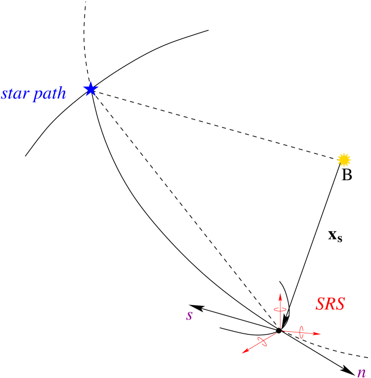
Figure 2: The vectors representing the light direction in the pM/pN approches inside the near-zone of the solar system.

From the property of a null trajectory and taking into account the metric which defines the BCRS it is

$$g_{\alpha\beta}p^{\alpha}p^{\beta}=0,$$

namely

$$\left[-1+\frac{\left(1+\gamma_{\mathrm{PPN}}\right)w(t,x)}{c^{2}}-\frac{2w^{2}(t,x)}{c^{4}}\right]+$$

$$2\delta_{ij}\left(-2\left(1+\gamma\mathrm{{}_{\mathrm{PPN}}}\right)\frac{w^{i}(t,x)}{c^{3}}\right)p^{j}+\delta_{ij}\left(1+\frac{\left(1+\gamma\mathrm{{}_{\mathrm{PPN}}}\right)w(t,x)}{c^{2}}\right)p^{i}p^{j} = 0$$

which gives

$$\frac{1}{p}=1+\frac{\left(1+\gamma\mathrm{{}_{\mathrm{PPN}}}\right)w(t,x)}{c^{2}}-\frac{2\left(1+\gamma\mathrm{{}_{\mathrm{PPN}}}\right)\delta_{ij}w^{i}(t,x)p^{j}}{c^{3}}+O(c^{-4})$$ (9)

where $p=\sqrt{\delta_{ij}p^{i}p^{j}}$ is the Euclidean modulus of the spatial vector $\mathbf{p}$ and $\gamma\mathrm{{}_{\mathrm{PPN}}}$ is the PPN parameter.

The infinitesimal transformation $\mathcal{X}^{\alpha}(x^{\beta})$ between CoMRS and BCRS is given by the formula:

$$\mathrm{d}\mathcal{X}^{\alpha}=\Lambda_{\beta}^{\alpha}\mathrm{d}x^{\beta}.$$ (10)

From (10) the expression of $s^{i}$ as a function of the spatial components $p^{i}$ is obtained:

$$s^{i}=-\frac{\Lambda_{0}^{i}+\Lambda_{j}^{i}p^{j}}{\Lambda_{0}^{0}+\Lambda_{j}^{0}p^{j}}.$$ (11)

One can explicit formula (11) by following the procedure reported in (Klioner and Kopeikin, 1992) and adopting the IAU resolution B1.3 (IAU, 2000). From the BCRS $\left(ct,x^{i}\right)$ to the CoMRS ($c\mathcal{T},\mathcal{X}^{i}$), the transformation between the time coordinates reads:

$$\mathcal{T} = t-c^{-2}[A(t)+\delta_{ij}v^{i}R_{\mathrm{s}}^{j}]$$

$$+c^{-4}[B+\delta_{ij}B^{i}R_{\mathrm{s}}^{j}+\delta_{im}\delta_{jk}B^{ij}R_{\mathrm{s}}^{m}R_{\mathrm{s}}^{k}+C(t,{\bf x})]+\mathcal{O}\left(c^{-5}\right),$$

and between the spatial coordinates

$$\mathcal{X}^{i}=\left[\delta_{j}^{i}+c^{-2}\left(\frac{1}{2}v^{i}v_{j}+qF_{j}^{i}(t)+D_{j}^{i}(t)\right)\right]R_{\mathrm{s}}^{j}+c^{-2}D_{jk}^{i}(t)R_{\mathrm{s}}^{j}R_{\mathrm{s}}^{k}+\mathcal{O}\left(c^{-4}\right).$$ (13)

All the functions $A,\,B,\,C,\,D$ are defined in Klioner and Kopeikin (1992) or in IAU resolutions and

$$R_{\mathrm{s}}^{i}=x^{i}-x_{\mathrm{s}}^{i}$$

are the coordinate displacements with respect to the center of mass of the satellite $x_{\mathrm{s}}^{i}$ in the BCRS, and finally

$$v^{i}=\frac{\mathrm{d}x_{\mathrm{s}}^{i}}{\mathrm{d}t}$$

is the coordinate velocity of the center of mass of the satellite relative to the BCRS.

As reported in Klioner (2004), the attitude in GREM (SRS) is obtained by applying an orthogonal rotation matrix $\mathcal{R}_{i}^{a}$ to $\mathcal{X}^{i}$ in equation (13). At this stage the role of the SRS is equivalent to that of the $E_{\hat{a}}^{\beta}$s in eq. (7).

If one keeps all the terms up to the order of 1 micro-arcsecond, the observed coordinate direction $s^{i}$, in terms of the unitary spatial vector $n^{i}=p^{i}/p$, becomes in the CoMRS:

$$s^{i} = -n^{i}+c^{-1}\left[\mathbf{n}\times\left(\mathbf{v}\times\mathbf{n}\right)\right]^{i}$$ (14)

$$+c^{-2}\left\{(\mathbf{n}\cdot\mathbf{v})\left[\mathbf{n}\times\left(\mathbf{n}\times\mathbf{v}\right)\right]^{i}+\frac{1}{2}\left[\mathbf{v}\times\left(\mathbf{n}\times\mathbf{v}\right)\right]^{i}\right\}$$

$$+c^{-3}\left\{\left[\left(\mathbf{v}\cdot\mathbf{n}\right)^{2}+(1+\gamma_{\mathrm{PPN}})w\left({\bf x_{\mathrm{s}}}\right)\right]\left[\mathbf{n}\times\left(\mathbf{v}\times\mathbf{n}\right)\right]^{i}\right.$$

$$\left.+\frac{1}{2}\left(\mathbf{n}\cdot\mathbf{v}\right)\left[\mathbf{\mathbf{v}}\times\left(\mathbf{n}\times\mathbf{v}\right)\right]^{i}\right\}+\mathcal{O}\left(\frac{v^{4}}{c^{4}}\right).$$

V RAMOD aberration in the PM approximation

Whatever tetrad we consider, the expression of Eq. (7) for the relativistic observable in the RAMOD model can also be written as (de Felice et al., 2006)

$$\mathbf{e}_{\hat{a}}=\frac{\left(\bar{l}_{\left(0\right)}-\nu\right)_{\beta}E_{\hat{a}}^{\beta}}{\gamma\left(1-\nu_{\alpha}\bar{l}_{\left(0\right)}^{\alpha}\right)},$$ (15)

where $\nu^{\alpha}$ is the spatial four-velocity (also called as the “physical velocity”) of the satellite $\mathbf{u^{\prime}}$ relative to the local baricentric observer $\mathbf{u}$. The quantity $\bar{l}_{\left(0\right)}^{\alpha}$ was introduced in RAMOD (de Felice et al., 2006) and is a unitary four-vector which represents the local line-of-sight of the photon as seen by $\mathbf{u}$, i.e. $\bar{l}_{(0)}^{\alpha}=P_{\beta}^{\alpha}(u)k^{\beta}$.

Finally, $\gamma$ is the Lorentz factor of $u^{\prime\alpha}$ with respect to $u^{\alpha}$, that is,

$$-u^{\prime\alpha}u_{\alpha}=\frac{1}{\sqrt{1-\nu^{2}/c^{2}}}\equiv\gamma,$$ (16)

where $\nu^{2}=\nu^{\alpha}\nu_{\alpha}$.

To retrieve the aberration effect given by the motion of the satellite with respect to the BCRS in RAMOD, one needs to specialize Eq. (15) to the case of a tetrad $\left\{\tilde{\lambda}_{\hat{\alpha}}\right\}$ adapted to the center of mass of the satellite assumed with no attitude parameters. In this case, in fact, the observation equation will give a relation between the “aberrated” direction represented by the direction cosines $\cos\psi_{a}$ as measured by the satellite and the “aberration-free” direction given by the quantity $\bar{l}_{\left(0\right)}^{\alpha}$ referred to the local BCRS frame $\lambda_{\hat{a}}^{\alpha}$. The vectors of the triad $\left\{\tilde{\lambda}_{\hat{a}}\right\}$ differ from the local BCRS’s $\left\{\lambda_{\hat{a}}\right\}$ for a boost transformation with four-velocity $u^{\prime\alpha}$. This means that it can be derived from Eq. (3) using the relation (Jantzen et al., 1992)

$$\tilde{\lambda}_{\hat{a}}^{\alpha}=P\left(u^{\prime}\right)_{\sigma}^{\alpha}\left[\lambda_{\hat{a}}^{\sigma}-\frac{\gamma}{\gamma+1}\nu^{\sigma}\left(\nu^{\rho}\lambda_{\rho\hat{a}}\right)\right],$$ (17)

where $u^{\prime\alpha}$ and $\nu^{\alpha}$ are the above mentioned four-velocity of the satellite and its physical velocity relative to the local BCRS respectively, and $P\left(u^{\prime}\right)_{\sigma}^{\alpha}=\delta_{\sigma}^{\alpha}+u^{\prime\alpha}u^{\prime}_{\sigma}$.

From de Felice et al. (2006) and Bini et al. (2003) it is

$$u^{\prime\alpha} = \left(1+\frac{U}{c^{2}}+\frac{1}{2}\frac{v^{2}}{c^{2}}\right)\left(\delta_{0}^{\alpha}+\frac{v^{i}}{c}\delta_{i}^{\alpha}\right)+\mathcal{O}\left(\frac{v^{4}}{c^{4}}\right)$$ (18)

where $v^{i}$ is the coordinate velocity of the satellite, as stated in the previous section. Now, being (de Felice et al., 2006)

$$\nu^{\alpha}=\frac{1}{\gamma}\left(u^{\prime\alpha}-\gamma u^{\alpha}\right),$$ (19)

one deduces that $\nu^{0}\sim\mathcal{O}\left(v^{4}/c^{4}\right)$ and

$$\nu^{i} = \left(1+\frac{U}{c^{2}}\right)\frac{v^{i}}{c}+\mathcal{O}\left(\frac{v^{4}}{c^{4}}\right).$$ (20)

Expanding Eq. (17) with relations (16) and (19) one gets

$$\tilde{\lambda}_{\hat{a}}^{\alpha} = \lambda_{\hat{a}}^{\alpha}+u^{\prime\alpha}\left(u^{\prime}|\lambda_{\hat{a}}\right)-\left(\frac{1}{2}+\frac{1}{8}\frac{v^{2}}{c^{2}}\right)\nu^{\alpha}\left(\nu|\lambda_{\hat{a}}\right)$$ (21)

$$- u^{\prime\alpha}\left(\frac{1}{2}+\frac{1}{8}\frac{v^{2}}{c^{2}}\right)\left(u^{\prime}|\nu\right)\left(\nu|\lambda_{\hat{a}}\right)+\mathcal{O}\left(\frac{v^{4}}{c^{4}}\right)$$

where the notation $\left(\cdot|\cdot\right)$ represents the scalar product, so, e.g., $\left(u^{\prime}|\lambda_{\hat{a}}\right)=g_{\alpha\beta}u^{\prime\alpha}\lambda_{\hat{a}}^{\beta}$.

Then, using Eqs. (3) (18) and (20) and expanding the scalar products to the right order we obtain

$$\left(u^{\prime}|\lambda_{\hat{a}}\right) = \left(1+\frac{2U}{c^{2}}+\frac{1}{2}\frac{v^{2}}{c^{2}}\right)\frac{v^{a}}{c}+\mathcal{O}\left(\frac{v^{4}}{c^{4}}\right)$$ (22)

$$\left(\nu|\lambda_{\hat{a}}\right) = \left(1+\frac{2U}{c^{2}}\right)\frac{v^{a}}{c}+\mathcal{O}\left(\frac{v^{4}}{c^{4}}\right)$$ (23)

$$\left(u^{\prime}|\nu\right) = \frac{v^{2}}{c^{2}}+\mathcal{O}\left(\frac{v^{4}}{c^{4}}\right)$$ (24)

so that the expression for the boosted tetrad finally becomes

$$\tilde{\lambda}_{\hat{a}}^{\alpha}=\lambda_{\hat{a}}^{\alpha}+\left(1+\frac{3U}{c^{2}}+\frac{1}{2}\frac{v^{2}}{c^{2}}\right)\delta_{0}^{\alpha}\frac{v^{a}}{c}+\frac{1}{2}\frac{v^{i}}{c}\delta_{i}^{\alpha}\frac{v^{a}}{c}+\mathcal{O}\left(\frac{v^{4}}{c^{4}}\right).$$ (25)

V.1 The $\left(v/c\right)^{3}$ expansion of the relativistic observable

Given Eq. (25) one can consistently recast Eq. (15) as

$$\mathbf{\tilde{e}}_{\hat{a}}=\frac{\left(\bar{l}-\nu\right)_{\beta}\lambda_{\hat{a}}^{\beta}}{\gamma\left(1-\nu_{\alpha}\bar{l}^{\alpha}\right)}+\frac{\left(\bar{l}-\nu\right)_{\beta}\delta_{0}^{\beta}}{\gamma\left(1-\nu_{\alpha}\bar{l}^{\alpha}\right)}\left(1+\frac{3U}{c^{2}}+\frac{1}{2}\frac{v^{2}}{c^{2}}\right)\frac{v^{a}}{c}+\frac{1}{2}\frac{\left(\bar{l}-\nu\right)_{\beta}\frac{v^{i}}{c}\delta_{i}^{\beta}}{\gamma\left(1-\nu_{\alpha}\bar{l}^{\alpha}\right)}\frac{v^{a}}{c}+\mathcal{O}\left(\frac{v^{4}}{c^{4}}\right)$$ (26)

where $\mathbf{\tilde{e}}_{\hat{a}}$ are the cosines related to the tetrad $\tilde{\lambda}_{\hat{a}}^{\alpha}$ which, as said, does not contain the attitude parameters. Here and in the rest of the section, we replace the symbol $\bar{l}_{\left(0\right)}^{\alpha}$ with $\bar{l}^{\alpha}$ to ease the notation.

After long calculations, the first term on the right-hand-side of this formula can be written as

$$\frac{\left(\bar{l}-\nu\right)_{\beta}\lambda_{\hat{a}}^{\beta}}{\gamma\left(1-\nu_{\alpha}\bar{l}^{\alpha}\right)} = \bar{l}^{a}+\frac{1}{c}\left[-v^{a}+\left(\delta_{ij}v^{i}\bar{l}^{j}\right)\bar{l}^{a}\right]+$$ (27)

$$\frac{1}{c^{2}}\left\{U\bar{l}^{a}-\left(\delta_{ij}v^{i}\bar{l}^{j}\right)v^{a}+\left[\left(\delta_{ij}v^{i}\bar{l}^{j}\right)^{2}-\frac{1}{2}v^{2}\right]\bar{l}^{a}\right\}+$$

$$\frac{1}{c^{3}}\left\{-2Uv^{a}-\left[\left(\delta_{ij}v^{i}\bar{l}^{j}\right)^{2}-\frac{1}{2}v^{2}\right]v^{a}+\right.$$

$$\phantom{\frac{1}{c^{3}}\{}\left.\bar{l}^{a}\left[3U\left(\delta_{ij}v^{i}\bar{l}^{j}\right)+\left(\delta_{ij}v^{i}\bar{l}^{j}\right)^{3}-\frac{1}{2}v^{2}\left(\delta_{ij}v^{i}\bar{l}^{j}\right)+U\left(\delta_{ij}v^{i}\bar{l}^{j}\right)\right]\right\}$$

$$+\mathcal{O}\left(\frac{v^{4}}{c^{4}}\right),$$

the second term is zero since both $\bar{l}_{0}$and $\nu_{0}$ are zero, while the third one becomes

$$\frac{1}{2}\frac{\left(\bar{l}-\nu\right)_{i}\left(v^{i}/c\right)}{\gamma\left(1-\nu_{\alpha}\bar{l}^{\alpha}\right)}\frac{v^{a}}{c} = \frac{1}{2}\left[\delta_{ij}\bar{l}^{i}\frac{v^{j}}{c}+\left(\delta_{ij}\frac{v^{i}}{c}\bar{l}^{j}\right)^{2}-\frac{v^{2}}{c^{2}}\right]\frac{v^{a}}{c}+\mathcal{O}\left(\frac{v^{4}}{c^{4}}\right).$$ (28)

Finally, collecting all terms:

$$\mathbf{\tilde{e}}_{\hat{a}} = \bar{l}^{a}+\frac{1}{c}\left[-v^{a}+\left(\delta_{ij}v^{i}\bar{l}^{j}\right)\bar{l}^{a}\right]+$$ (29)

$$\frac{1}{c^{2}}\left\{U\bar{l}^{a}-\frac{1}{2}\left(\delta_{ij}v^{i}\bar{l}^{j}\right)v^{a}+\left[\left(\delta_{ij}v^{i}\bar{l}^{j}\right)^{2}-\frac{1}{2}v^{2}\right]\bar{l}^{a}\right\}+$$

$$\frac{1}{c^{3}}\left\{-2Uv^{a}-\frac{1}{2}\left(\delta_{ij}v^{i}\bar{l}^{j}\right)^{2}v^{a}+\right.$$

$$\phantom{\frac{1}{c^{3}}\{}\left.\bar{l}^{a}\left[3U\left(\delta_{ij}v^{i}\bar{l}^{j}\right)+\left(\delta_{ij}v^{i}\bar{l}^{j}\right)^{3}-\frac{1}{2}v^{2}\left(\delta_{ij}v^{i}\bar{l}^{j}\right)+U\left(\delta_{ij}v^{i}\bar{l}^{j}\right)\right]\right\}+\mathcal{O}\left(\frac{v^{4}}{c^{4}}\right).$$

At a first glance, the last expression shows differences in terms up to the $\left(v/c\right)^{2}$ order (note in particular the appearance of the term $U\bar{l}^{a}$) and of the $\left(v/c\right)^{3}$ order which cannot allow to straightforwardly compare, as expected, the above expression to the GREM vectorial one of Eq. (14).

V.2 Comparison with the GREM model

The expression (29) relates the observed direction cosines with $\bar{l}^{\alpha}$. The equivalent relation for the GREM observable is equation (14) where the aberration is expressed in terms of a vector $\mathbf{n}$. To compare formula (29) with GREM’s formula (14) we need to find a relationship between $\mathbf{n}$ and $\bar{l}^{\alpha}$. To this purpose we need to reduce $\bar{l}^{\alpha}$ to its coordinate euclidean expression

In GREM $\mathbf{n}$ represents the “aberration-free” coordinate line of sight of the observed star at the position of the satellite momentarily at rest. In RAMOD, as said, $\bar{l}^{\alpha}$ represents the normalized local line-of-sight of the observed star as seen by the local barycentric observer $\mathbf{u}$. In other words, $\bar{l}^{\alpha}$ is a four-vector which fixes the line-of-sight of an object with respect to the local BCRS.

Do $\mathbf{n}$ and $\bar{l}^{\alpha}$ have a similar role in the two approaches? From the physical point of view they have the same meaning, as the observed “aberration free” direction to the star. Let us start from the definition of $\mathbf{n}$ in GREM:

$$n^{i}=\frac{p^{i}}{p},$$

where $p^{i}=c^{-1}\mathrm{d}x^{i}/\mathrm{d}t$ and $p$ is the Euclidean norm of $p^{i}$, so that $p^{-1}\simeq\left(1+h_{00}+h_{0i}p^{i}\right)+\mathcal{O}\left(h^{2}\right)$, as equation (9) shows. This means that

$$n^{i}=p^{i}\left(1+h_{00}+h_{0i}p^{i}\right)+\mathcal{O}\left(h^{2}\right).$$ (30)

On the other hand, using the definition of $\bar{l}^{\alpha}$ in de Felice et al. (2006) it can be easily shown that its spatial components are

$$\bar{l}^{i}=-\frac{k^{i}}{u_{\alpha}k^{\alpha}}=-\frac{k^{i}}{u^{0}k^{0}\left(-1+h_{00}+h_{0i}\frac{k^{i}}{k^{0}}\right)},$$

and, from $u^{0}=\left(-g_{00}\right)^{-1/2}$ and $k^{i}/k^{0}=c^{-1}\mathrm{d}x^{i}/\mathrm{d}t\equiv p^{i}$, it results

$$\bar{l}^{i} = p^{i}\left(-g_{00}\right)^{1/2}\left(1-h_{00}-h_{0i}p^{i}\right)^{-1}$$ (31)

$$= p^{i}\left(1+\frac{1}{2}h_{00}+h_{0i}p^{i}\right)+\mathcal{O}\left(h^{2}\right).$$

Finally, from equations (30) and (31) one has

$$\bar{l}^{i} = n^{i}\left(1-\frac{U}{c^{2}}\right)+\mathcal{O}\left(\frac{v^{4}}{c^{4}}\right)$$ (32)

namely, the spatial light direction, expressed in terms of its Euclidean counterpart at the satellite location in the gravitational field of the solar system. Worth noticing is that no terms of the order of $\mathcal{O}[(v/c)^{3}]$ appear in (32).

Combining Eq. (29) with (32) and setting $\left(\delta_{ij}v^{i}n^{j}\right)\equiv\mathbf{v}\cdot\mathbf{n}$ to ease the notation, we obtained

$$\mathbf{\tilde{e}}_{\hat{a}} = n^{a}+\frac{1}{c}\left[-v^{a}+\left(\mathbf{v}\cdot\mathbf{n}\right)n^{a}\right]+\frac{1}{c^{2}}\left\{-\frac{1}{2}\left(\mathbf{v}\cdot\mathbf{n}\right)v^{a}+\left[\left(\mathbf{v}\cdot\mathbf{n}\right)^{2}-\frac{1}{2}v^{2}\right]n^{a}\right\}+$$ (33)

$$\frac{1}{c^{3}}\left\{-2Uv^{a}-\frac{1}{2}\left(\mathbf{v}\cdot\mathbf{n}\right)^{2}v^{a}+\left(\mathbf{v}\cdot\mathbf{n}\right)n^{a}\left[2U+\left(\mathbf{v}\cdot\mathbf{n}\right)^{2}-\frac{1}{2}v^{2}\right]\right\}+\mathcal{O}\left(\frac{v^{4}}{c^{4}}\right).$$

In this way the right-hand side of the aberration expression of RAMOD is rewritten with the GREM quantities at the $\left(v/c\right)^{3}$ order. The same operation can be done for the left-hand side using the definition of the projection operator and the tetrad property $\lambda_{\alpha}^{\hat{\mu}}\lambda_{\hat{\mu}\beta}=g_{\alpha\beta}$:

$$\mathbf{\tilde{e}}_{\hat{a}}\equiv\frac{P(u)_{\alpha\beta}k^{\alpha}\tilde{\lambda}_{\hat{a}}^{\beta}}{\left(P(u)_{\alpha\beta}k^{\alpha}k^{\beta}\right)^{1/2}}=\frac{k^{\alpha}\tilde{\lambda}_{\alpha}^{\hat{a}}}{|g_{\alpha\beta}u^{\alpha}k^{\beta}|}=-\frac{k^{\alpha}\tilde{\lambda}_{\alpha}^{\hat{a}}}{g_{\alpha\beta}\tilde{\lambda}_{\hat{0}}^{\alpha}k^{\beta}}=\frac{k^{\alpha}\tilde{\lambda}_{\alpha}^{\hat{a}}}{k^{\beta}\tilde{\lambda}_{\beta}^{\hat{0}}}=\frac{\mathrm{d}\tilde{x}^{\hat{a}}}{\mathrm{d}\tilde{x}^{\hat{0}}}.$$ (34)

Is there a relation between the direction cosines of the above equation with the spatial components of the observed vector $s^{i}$ in GREM? The crucial point stands on the definition of the coordinates system. The tetrad components of the light ray can be directly associated to CoMRS coordinates (as done in Klioner (2004)) if the boosted local BCRS tetrad coordinates $\tilde{x}^{\hat{\alpha}}$ are equivalent to the CoMRS ones $\mathcal{X}^{\alpha}$. This is true only locally, i.e. in a sufficiently small neighborhood (since the tetrad are not in general olonomous) and if the origins of the two reference systems concide. So, from (8), if one could state that

$$\frac{\mathrm{d}\tilde{x}^{\hat{a}}}{\mathrm{d}\tilde{x}^{\hat{0}}}=\frac{\mathrm{d}\mathcal{X}^{a}}{\mathrm{d}\mathcal{X}^{0}}\equiv-s^{a},$$

it would follow

$$\mathbf{\tilde{e}}_{\hat{a}}=-s^{a}.$$ (35)

In RAMOD, at the milli-arcsecond level, the rest space of the local baricentric observer coincides globally with the spatial hypersurfaces which foliate the space-time and define the BCRS (de Felice et al., 2004). At micro-arcsecond accuracy, instead, the vorticity cannot be neglected and the geometry is affected by non-diagonal terms of the metric hence the $t=\mathrm{constant}$ hypersurfaces do not coincide with the rest-space of the local barycentric observer (de Felice et al., 2006). Then, to be consistent we can only define at each point of observation a spatial direction measured by the local barycentric observer and then associate it to the satellite measurements via the direction cosines relative to the boosted attitude frame. As far as GREM is concerned, the euclidean geometry admits a parallel transport which does not feel the curvature, allowing to define the same vector in any point of the space.

Then, equation (35) has only local validity and (33)can be written as

$$-s^{a} = n^{a}+\frac{1}{c}\left[-v^{a}+\left(\mathbf{v}\cdot\mathbf{n}\right)n^{a}\right]+\frac{1}{c^{2}}\left\{-\frac{1}{2}\left(\mathbf{v}\cdot\mathbf{n}\right)v^{a}+\left[\left(\mathbf{v}\cdot\mathbf{n}\right)^{2}-\frac{1}{2}v^{2}\right]n^{a}\right\}+$$ (36)

$$\frac{1}{c^{3}}\left\{-2Uv^{a}-\frac{1}{2}\left(\mathbf{v}\cdot\mathbf{n}\right)^{2}v^{a}+\left(\mathbf{v}\cdot\mathbf{n}\right)n^{a}\left[2U+\left(\mathbf{v}\cdot\mathbf{n}\right)^{2}-\frac{1}{2}v^{2}\right]\right\}+\mathcal{O}\left(\frac{v^{4}}{c^{4}}\right).$$

Considering that $\mathbf{n}\cdot\mathbf{n}=1$ and $v^{2}=\delta_{ij}v^{i}v^{j}\equiv\mathbf{v}\cdot\mathbf{v}$, the previous equation becomes

$$s^{a} = -n^{a}+\frac{1}{c}\left[v^{a}\left(\mathbf{n}\cdot\mathbf{n}\right)-n^{a}\left(\mathbf{v}\cdot\mathbf{n}\right)\right]+$$ (37)

$$\frac{1}{c^{2}}\left\{\left(\mathbf{v}\cdot\mathbf{n}\right)\left[v^{a}\left(\mathbf{n}\cdot\mathbf{n}\right)-n^{a}\left(\mathbf{v}\cdot\mathbf{n}\right)\right]+\frac{1}{2}\left[n^{a}\left(\mathbf{v}\cdot\mathbf{v}\right)-v^{a}\left(\mathbf{v}\cdot\mathbf{n}\right)\right]\right\}+$$

$$\frac{1}{c^{3}}\left\{2U\left[v^{a}\left(\mathbf{n}\cdot\mathbf{n}\right)-n^{a}\left(\mathbf{v}\cdot\mathbf{n}\right)\right]+\left(\mathbf{v}\cdot\mathbf{n}\right)^{2}\left[v^{a}\left(\mathbf{n}\cdot\mathbf{n}\right)-n^{a}\left(\mathbf{v}\cdot\mathbf{n}\right)\right]+\right.$$

$$\phantom{\frac{1}{c^{3}}\{}\left.\frac{1}{2}\left(\mathbf{v}\cdot\mathbf{n}\right)\left[n^{a}\left(\mathbf{v}\cdot\mathbf{v}\right)-v^{a}\left(\mathbf{v}\cdot\mathbf{n}\right)\right]\right\}+\mathcal{O}\left(\frac{v^{4}}{c^{4}}\right).$$

Finally, from the relation $\mathbf{a}\times\left(\mathbf{b}\times\mathbf{c}\right)=\mathbf{b}\left(\mathbf{a}\cdot\mathbf{c}\right)-\mathbf{c}\left(\mathbf{a}\cdot\mathbf{b}\right)$ it is

$$s^{a} = -n^{a}+\frac{1}{c}\left[\mathbf{n}\times\left(\mathbf{v}\times\mathbf{n}\right)\right]^{a}+\frac{1}{c^{2}}\left\{\left(\mathbf{v}\cdot\mathbf{n}\right)\left[\mathbf{n}\times\left(\mathbf{v}\times\mathbf{n}\right)\right]^{a}+\frac{1}{2}\left[\mathbf{v}\times\left(\mathbf{n}\times\mathbf{v}\right)\right]^{a}\right\}+$$ (38)

$$\frac{1}{c^{3}}\left\{\left[\left(\mathbf{v}\cdot\mathbf{n}\right)^{2}+2U\right]\left[\mathbf{n}\times\left(\mathbf{v}\times\mathbf{n}\right)\right]^{a}+\frac{1}{2}\left(\mathbf{v}\cdot\mathbf{n}\right)\left[\mathbf{v}\times\left(\mathbf{n}\times\mathbf{v}\right)\right]^{a}\right\}+\mathcal{O}\left(\frac{v^{4}}{c^{4}}\right)$$

which is formula(14) for the aberration in GREM if we consider the case of GR where $\gamma\mathrm{{}_{\mathrm{PPN}}}=1$ and we take into account that $\mathbf{v}\equiv\dot{\mathbf{x}}_{\mathrm{o}}$, and $U\equiv w\left(\mathbf{x}_{\mathrm{o}}\right)$.

Finally, the result obtained with eq. (38) states that, limited to the case of aberration and using the appropriate definitions of the IAU recommendations, RAMOD recovers GREM at the $\left(v/c\right)^{3}$ order.

VI Conclusions

This paper compares two relativistic astrometric models, GREM and RAMOD, both suitable for modelling modern astrometric observations at the micro-arcsecond accuracy. Their different mathematical structures hinder a straightforward comparison and call for a more in-depth analysis of the two models. Because of the structure of GREM, the earliest stage of a theoretical comparison starts with the evaluation of the aberration “effect” in RAMOD. In this regard, we can evidence the following differences in: (i) the choice of the boundary conditions, (ii) the tools needed to define the astrometric measurements, (iii) the attitude implementation, (iv) the definition of the proper light direction.

Crucial is point (i). The light signal arriving at the local BCRS along the spatial direction $l^{\alpha}=P(u)_{\beta}^{\alpha}k^{\beta}$ satisfies the RAMOD master equations, namely a set of non-linear coupled differential equations (de Felice et al., 2006). Therefore the cosines (i.e. the astrometric measurements) taken as a function of the local line-of-sight (the physical one), at the time of observation ($l_{(0)}^{i}$), allow to fix the boundary conditions needed to solve the master equations and to determine uniquely the star coordinates. However, since the direction cosines are expressed in terms of the attitude, the mathematical characterization of the attitude frame is essential to complete the boundary value problem in the process of reconstructing the light trajectory. The vector $\mathbf{n}$, i.e. the “aberration-free” counterpart of $l^{\alpha}$ in GREM, is instead used to derive the aberration effect (in a coordinate language) and there is no need to connect it with a RAMOD-like boundary value problem.

As for the solution of the geodesic equation, RAMOD defines a complete procedure to derive the satellite attitude which depends as input only on the specific terms of the metric that describes the addressed physical problem. GREM, instead, embeds the definitions of its main reference system (BCRS) within the metric, consequently each further step depends on this choice. This includes all the subsequents transformations among the reference systems which are essential to extract the GREM observable as function of the astrometric unknowns. On the other side, the RAMOD analytical solution for the attitude frame assures controlled alghoritms that can be directly implemented in the solution of the astrometric problem and guarantee its consistency with GR. In RAMOD the direction cosines link the attitude of the satellite to the measurements, compacting several reference frames useful to determine, as final task, the stellar coordinates: the BCRS (kinematically non-rotating global reference rame), the CoMRS (a local reference frame comoving with the satellite centre of mass), and the SRS (the attitude triad of the satellite). The coordinate transformations between BCRS/CoMRS/SRS come out naturally once the IAU conventions are adopted. This is inside the conceptual framework of RAMOD, where the astrometric set-up allows to trace back the light ray to the emitting star in a curved geometry, and it is not natural to disentangle each single effect. Any approximation can be applied a posteriori where it is needed, case by case. This explains items (ii) and (iii) and introduces item (iv).

The direction cosines being physical quantities not depending on the coordinates, are a powerful tool to compare the astrometric relativistic models: their physical meaning allow us to correctly intepret the astrometric parameters in terms of coordinate quantities. This justified the conversion of the physical stellar proper direction of RAMOD into its analgous Euclidean coordinate counterpart, which ultimately leads to the derivation of a GREM-style aberration formula. Another point arises when the observables of RAMOD have to be identified with components of the observed $s^{i}$ of GREM. This matching is admitted only if the origins of the boosted local BCRS tetrad in RAMOD and of the CoMRS in GREM concide.

To what extent the process of star coordinate “reconstruction” is consistent with GR&Theory of Measurements? Solving the astrometric problem in practice means to compile an astrometric catalogue at same order of accuracy of the measurements. This paper shows that, already at the level of the aberration effect, a correct treatment of physical meaurements in terms of coordinate quantities needs particular care in order to avoid misunderstandings in the interpretation of the quantities which constitute the final catalogue.

As a closing consideration, the computation of the BCRS stellar direction in GREM needs to extract, at a second stage, the deflection terms from the coordinate “aberration-free” direction $n^{i}$ . This problem in RAMOD is, again, embedded in the formulation of the astrometric problem as “global solution” which aims at recovering the star coordinates by integration of the geodesic equations (treated with an appropriate physical boundary condition and approriate reference systems) where the deflection terms play the most fundamental role.