Zero Sound and First Sound in a Disk-Shaped Normal Fermi gas

Abstract

We study the zero sound and the first sound in a dilute and ultracold disk-shaped normal Fermi gas with a strong harmonic confinement along the axial direction and uniform in the two planar directions. Working at zero temperature we calculate the chemical potential $\mu$ of the fermionic fluid as a function of the uniform planar density $\rho$ and find that $\mu$ changes its slope in correspondence to the filling of harmonic axial modes (shell effects). Within the linear response theory, and under the random phase approximation, we calculate the velocity $c^{0}_{s}$ of the zero sound. We find that also $c^{0}_{s}$ changes its slope in correspondence of the filling of the harmonic axial modes and that this effect depends on the Fermi-Fermi scattering length $a_{F}$. In the collisional regime, we calculate the velocity $c_{s}$ of first sound showing that $c_{s}$ displays jumps at critical densities fixed by the scattering length $a_{F}$. Finally, we discuss the experimental achievability of these zero sound and first sound waves with ultracold alkali-metal atoms.

I Introduction

Effects of quantum statistics are observable with both bosonic book-pethick ; book-stringari and fermionic demarco ; truscott ; modugno ; greiner ; joachim vapors of alkali-metal atoms at ultra-low temperatures. In these quantum degenerate gases, the role of dimensionality has been experimentally studied with bosons gorlitz ; schreck ; kinoshita , while for fermions, there are only theoretical predictions. In particular, it has been suggested that a reduced dimensionality strongly modifies density profiles schneider ; sala0 ; sala1 ; vignolo , collective modes bruun ; minguzzi and stability of mixtures das ; sala2 . Also sound velocities have been theoretically investigated in reduced dimensions for both normal minguzzi ; capuzzi1 and superfluid Fermi gases ghosh ; capuzzi2 ; capuzzi3 .

It has been shown that, in the weak coupling limit, the zero sound velocity $c_{s}^{0}$ and the first sound velocity $c_{s}$ of a normal Fermi gas are equal in the strictly one-dimensional (1D) geometry minguzzi , contrary to the 3D case where they differ by a factor $\sqrt{3}$ if the system is uniform landau ; pines ; fetter , or by a factor $\sqrt{5}$ if the system is cigar-shaped due to a isotropic harmonic confinement in two directions capuzzi1 . Very recently we have studied the first sound velocity $c_{s}$ of a normal cigar-shaped Fermi gas in the 1D to 3D crossover, showing that $c_{s}$ exhibits jumps in correspondence of the filling of planar harmonic shells sala-reduce1 .

In this paper we investigate, at zero temperature, the zero sound velocity $c_{s}^{0}$ and the first sound velocity $c_{s}$ of a normal Fermi gas in the dimensional crossover from 2D to 3D by considering a harmonic confinement in the axial direction. We show that by increasing the planar density $\rho$ of fermions (or equivalently the chemical potential $\mu$) one induces the dimensional crossover in the system. In general, collective sound modes in a normal Fermi system are of two kinds. When the collision time $\tau$ between quasiparticles is much greater than the period ($\omega^{-1}$) of the mode itself, i.e. if $\omega\tau\gg 1$, the system is in the so-called collisionless regime. In presence of a repulsive interaction, the resulting collective mode is known as zero sound landau ; pines ; fetter ; negele ; vignale ; lipparini . In the present work we approach the problem calculating the density-density response function in the random-phase approximation. The poles of this response function lead to the zero sound dispersion law and to its velocity of propagation $c_{s}^{0}$ in the radial plane, where the gas is not confined. We investigate the behavior of the zero sound velocity $c_{s}^{0}$ as a function of the chemical potential, or, equivalently, of the fermionic density in the transverse radial plane.

When collisions between atoms are characterized by a sufficiently small collision time such that $\omega\tau\ll 1$, the system may be assumed to be at thermal equilibrium. In this regime, the Fermi fluid is accurately described by quantum hydrodynamics equations where the fermionic nature appears in the bulk equation of state landau ; fetter ; negele . In this case, the collective mode is called first sound (or ordinary sound, or collisional sound). The first sound velocity $c_{s}$ has been studied previously both in the 1D-3D and 2D-3D crossovers sala-reduce2 ; sala-reduce3 , and in a 3D cylindrical geometry zaremba for an ultracold Bose gas. It is important to stress that the propagation of ordinary sound in spin unpolarized Fermi gases may be studied also from the experimental point of view. For instance, Joseph and co-workers joseph were able to excite first sound waves in an optically trapped Fermi degenerate gas of spin-up and spin-down atoms by using magnetically tunable interactions. In this paper we predict that, as in the 1D-3D crossover sala-reduce1 , the first sound velocity $c_{s}$ displays observable shell effects in the 2D-3D crossover of a disk-shaped ultracold Fermi gas. By increasing the planar density $\rho$, that is by inducing the crossover from two-dimensions to three-dimensions, $c_{s}$ shows jumps in correspondence of the filling of harmonic modes. Such jumps of the sound velocity, even if less pronounced than the ones predicted in the 1D-3D crossover sala-reduce1 , can be experimentally observed.

In the last part of the paper we establish the experimental conditions to be achieved for detecting zero sound and first sound. In particular, by considering ⁴⁰K atoms, we estimate the critical mode frequency $\omega_{c}$ which discriminates between the collisional and the collisionless regimes.

II Confined interacting Fermi gas

We consider an ultracold normal Fermi gas with two-spin components confined by a harmonic trap in the axial direction and investigate the regime where the temperature $T$ of the gas is well below the Fermi temperature $T_{F}$ so that we may use a zero-temperature approach and treat separately the collisionless and the collisional regimes. The Hamiltonian of the dilute Fermi gas trapped by the external harmonic potential

$$U({\bf r})=\displaystyle{\frac{1}{2}m\omega_{z}^{2}z^{2}}\;,$$ (1)

and free to move in the $(x,y)$ plane in a square box of size $L$, is given by

$$\hat{H}=\sum_{\sigma=\uparrow,\downarrow}\int d{\bf r}\hat{\Psi}^{\dagger}_{\sigma}({\bf r})\bigg{(}-\frac{\hbar^{2}}{2m}\nabla^{2}+U({\bf r})\bigg{)}\hat{\Psi}_{\sigma}({\bf r})$$

$$+ \frac{g_{F}}{2}\sum_{\sigma,\sigma^{\prime}=\uparrow,\downarrow}\int d{\bf r}\hat{\Psi}^{\dagger}_{\sigma}({\bf r})\hat{\Psi}^{\dagger}_{\sigma^{{}^{\prime}}}({\bf r})\hat{\Psi}_{\sigma^{{}^{\prime}}}({\bf r})\hat{\Psi}_{\sigma}({\bf r})(1-\delta_{\sigma,\sigma^{\prime}})\;,$$

where $\sigma=\{\uparrow,\downarrow\}$ denotes the spin variable, and the inter-atomic coupling is

$$g_{F}=4\pi\hbar^{2}a_{F}/m\;,$$ (2)

with $a_{F}>0$ being the $s$-wave scattering length. ${\hat{\Psi}}_{\sigma}({\bf r})$ and ${\hat{\Psi}}_{\sigma}^{\dagger}({\bf r})$ are the usual operators annihilating or creating a fermion of spin $\sigma$ at the position ${\bf r}$, therefore obeying anticommutation relations landau ; pines ; fetter ; negele . The field operator can be written as

$${\hat{\Psi}}_{\sigma}({\bf r})=\sum_{\alpha}\phi_{\alpha}({\bf r})\,{\hat{c}}_{\sigma,{\alpha}}$$ (3)

in terms of the single-particle operators ${\hat{c}}_{\sigma,\alpha}$ (${\hat{c}}^{\dagger}_{\sigma,\alpha}$) destroying (creating) a fermion of spin $\sigma$ with the single-particle wave function $\phi_{\alpha}({\bf r})$. Because of the symmetry of the problem, $\phi_{\alpha}({\bf r})$ can be factorized into the product of eigenfunctions of the harmonic oscillator in the $z$ direction and plane waves describing free motion in the $(x,y)$ plane. The field operator, then, may be written as

$$\hat{\Psi}_{\sigma}({\bf r})=\frac{1}{L^{2}}\sum_{j,{\bf K}}\psi_{j}(z)\exp(i{\bf K}\cdot{\bf R})\hat{c}_{\sigma,j,{\bf K}}\;$$ (4)

with ${\bf R}\equiv(x,y)$, and where $\psi_{m}(z)$ is the real function

$$\psi_{j}(z)=\sqrt{\frac{1}{2^{j}j!\pi^{1/2}a_{z}}}H_{j}(\frac{z}{a_{z}})\exp(-z^{2}/2a_{z}^{2})\;.$$ (5)

$\displaystyle{H_{j}(\frac{z}{a_{z}})}$ is the $j$-th Hermite polynomial of argument $z/a_{z}$, $a_{z}=\sqrt{\hbar/(m\omega_{z})}$ being the characteristic length of the axial harmonic potential.

The two dimensional wave vector ${\bf K}\equiv(K_{x},K_{y})$ embeds the translational invariance in the radial plane. By imposing periodic boundary conditions in the box of length $L$ along $x$ and $y$ directions, the components $K_{x}$ and $K_{y}$ of ${\bf K}$ are quantized according to: $\displaystyle{K_{x}=\frac{2\pi}{L}{i_{x}}}$ and $\displaystyle{K_{y}=\frac{2\pi}{L}{i_{y}}}$, where $i_{x}$ and $i_{y}$ are integer quantum numbers. The index $\alpha$ reads $(j,K_{x},K_{y})$, or in a more compact form $(j,{\bf K})$.

By inserting Eq. (4) into (II) the Hamiltonian takes the form

$$\hat{H}=\hat{H}_{0}+\hat{H}_{int}\;,$$ (6)

where

$$\hat{H}_{0}=\sum_{\sigma,j,{\bf K}}\epsilon^{0}_{j,{\bf K}}\hat{c}^{\dagger}_{\sigma,j,\bf K}\hat{c}_{\sigma,j,\bf K}\;,$$ (7)

and

$$\hat{H}_{int}=\frac{g_{F}}{2a_{z}L^{2}}\sum_{\sigma,\sigma^{\prime}}\sum_{j_{1},j_{2},j_{3},j_{4}}\sum_{\bf K_{1},\bf K_{2},\bf Q}W_{j_{1},j_{2},j_{3},j_{4}}$$

$$\hat{c}^{\dagger}_{\sigma,j_{1},\bf K_{1}+\bf Q}\hat{c}^{\dagger}_{\sigma^{\prime},j_{2},{\bf K_{2}}-\bf Q}\hat{c}_{\sigma^{\prime},j_{3},{\bf K_{2}}}\hat{c}_{\sigma,j_{4},{\bf K_{1}}}(1-\delta_{\sigma,\sigma^{\prime}})\;,$$

with

$$\epsilon^{0}_{j,\bf K}=\frac{\hbar^{2}K^{2}}{2m}+(j+\frac{1}{2})\hbar\omega_{z}\;,$$ (9)

and

$$W_{j_{1},j_{2},j_{3},j_{4}}=\bigg{(}\frac{1}{\pi}\prod_{j_{i},i=1}^{4}\sqrt{\frac{1}{2^{j_{i}}j_{i}!}}\bigg{)}$$

$$\int_{-\infty}^{+\infty}d\xi e^{-2\xi^{2}}H^{*}_{j_{1}}(\xi)H^{*}_{j_{2}}(\xi)H_{j_{3}}(\xi)H_{j_{4}}(\xi).$$ (10)

Eq. (9) gives the single-particle energies of noninteracting fermions. To obtain the single-particle energies of interacting fermions we calculate the two-spin Green function

$$G^{\sigma,\sigma^{\prime}}_{j_{1},j_{2},{\bf K}}(t-t^{\prime})=-\frac{i}{\hbar}\langle T\big{(}\hat{c}_{\sigma,j_{1},\bf K}(t)\hat{c}^{\dagger}_{\sigma^{\prime},j_{2},\bf K}(t^{\prime})\big{)}\rangle\;$$ (11)

where $T$ denotes the time ordering operator. Here and in the following, we will represent the operators in the interaction picture (with $\hat{H}_{0}$ the unperturbed Hamiltonian), and will evaluate the averages with respect to the ground state of the Hamiltonian (6). In the calculation of the Green function we use a mean field approach and replace the four operators terms involved in $\hat{H}_{int}$ with $\langle\hat{c}^{\dagger}_{\sigma,j_{1},\bf K_{1}+\bf Q}\hat{c}_{\sigma,j_{4},{\bf K_{1}}}\rangle\hat{c}^{\dagger}_{\sigma^{\prime},j_{2},\bf K_{2}-\bf Q}\hat{c}_{\sigma^{\prime},j_{3},{\bf K_{2}}}+\hat{c}^{\dagger}_{\sigma,j_{1},\bf K_{1}+\bf Q}\hat{c}_{\sigma,j_{4},{\bf K_{1}}}\langle\hat{c}^{\dagger}_{\sigma^{\prime},j_{2},{\bf K_{2}}-\bf Q}\hat{c}_{\sigma^{\prime},j_{3},{\bf K_{2}}}\rangle$. The poles of the Green function with $\sigma=\sigma^{\prime}$ and $j_{1}=j_{2}=j$ give directly the single-particle energies $\epsilon_{j,{\bf K}}$ of the interacting fermions

$$\epsilon_{j,{\bf K}}=\frac{\hbar^{2}K^{2}}{2m}+(j+\frac{1}{2})\hbar\omega_{z}+\frac{g_{F}}{2a_{z}L^{2}}\;\sum_{l=0}^{l_{max}}u_{j,l}{n}_{l}$$

where

$${n}_{l}=\sum_{{\bf K},\sigma}\langle\hat{c}^{\dagger}_{\sigma,l,{\bf K}}\hat{c}_{\sigma,l,{\bf K}}\rangle\;$$ (13)

is the total number of fermions in the harmonic shell $l$ and $u_{j,l}=u_{l,j}=W_{l,l,j,j}$ is obtained from Eq. (10).

In Tab. 1 we report the numerical values of the coefficients $u_{l,j}$ for $l$ and $j$ up to $4$.

The maximum positive integer $l_{max}$ involved in the summation at the right hand side of Eq. (II) clearly depends on the single-particle state $(j,{\bf K})$ and on the interaction strength $g_{F}$.

If spin-up and spin-down states are equally populated we may write the total number of fermions in the $l$-th harmonic state as

$${n}_{l}=2\,\sum_{{\bf K}}\,\Theta(\bar{\mu}-\epsilon_{l,{\bf K}})\;.$$ (14)

with $\bar{\mu}$ the chemical potential, i.e. the Fermi energy.

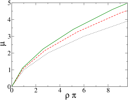
Figure 1: (Color online). Chemical potential $\mu$ vs. planar density $\rho$. Three values of the scaled interaction strength: $g=10^{-5}$ (dotted curve), $g=0.35$ (dashed curve), $g=0.6$ (solid curve). The chemical potential is in units of $\hbar\omega_{z}$, density in units of $1/a_{z}^{2}$, and lengths in units of $a_{z}$.

From here we may calculate the 2D fermion density in the $(x,y)$ plane as a function of the chemical potential. Under the condition $L\gg a_{z}$ on the planar box size, the summation over $\bf K$ may be repaced by an integral to get the 2D density associated to the $j$th axial mode, which is uniform in the $(x,y)$ plane and is given by

$${}\rho_{j}={{n}_{j}\over L^{2}}=2\frac{1}{(2\pi)^{2}}\int d^{2}{\bf K}\,\Theta(\bar{\mu}-\epsilon_{j,{\bf K}})\;.$$ (15)

$(l,j)$	$u_{l,j}\ \sqrt{2\pi}$
$(0,0)$	$1$
$(0,1)$	${1/2}$
$(0,2)$	${3/8}$
$(0,3)$	${5/16}$
$(0,4)$	${35/128}$
$(1,1)$	${3/4}$
$(1,2)$	${7/16}$
$(1,3)$	${11/32}$
$(1,4)$	${75/256}$
$(2,2)$	${41/64}$
$(2,3)$	${51/128}$
$(2,4)$	${329/1024}$
$(3,3)$	${147/256}$
$(3,4)$	${759/2048}$
$(4,4)$	${8649/16384}$

Table 1. Coefficients $u_{l,j}$. Note that $u_{l,j}=u_{j,l}$.

If only only the lowest ($j=0$) single-particle mode along the $z$ axis is occupied, then the system may be considered as strictly 2D. After inserting Eq. (II) into Eq. (15) an easy integration gives

$$\rho_{j}=\frac{m}{\pi\hbar^{2}}(\mu-\hbar\omega_{z}j-\frac{g_{F}}{2a_{z}}\sum_{l=0}^{l_{max}}u_{j,l}\rho_{l})\;,$$ (16)

where

$$\mu=\bar{\mu}-\frac{\hbar\omega_{z}}{2}\;$$ (17)

is the chemical potential measured with respect to the ground state energy of the axial harmonic potential. The expression (16) may be rewritten as

$$\sum_{l=0}^{l_{max}}\big{(}\delta_{j,l}+gu_{j,l}\big{)}\rho_{l}=\frac{m}{\pi\hbar^{2}}(\mu-\hbar\omega_{z}j)\;,$$ (18)

where

$$g=\frac{g_{F}}{2\pi\hbar\omega_{z}a_{z}^{3}}={2a_{F}\over a_{z}}\>$$ (19)

is the scaled inter-atomic strength.

The total planar density is then given by

$$\rho=\sum_{l=0}^{l_{max}}\rho_{l}\;,$$ (20)

where the only nonzero densities $\rho_{0},\rho_{1},...,\rho_{l_{max}-1},\rho_{l_{max}}$ are obtained by solving the ${l_{max}}+1$ Eqs. (18) at fixed $\mu$ and $g$. The value of $l_{max}$ is determined by requiring that all the $l_{max}+1$ solutions are positive. Note that when only $\rho_{0}$ is non zero, we have a strictly 2D system. In Fig.1 we plot the chemical potential $\mu$ as a function of the planar density $\rho$ for three values of the scaled interaction strength $g$. The figure shows the changes in the slope of these curves which occur when the planar density is sufficiently large so that a new excited level of the axial harmonic well (a new shell) begins to be populated.

III Zero sound

In the present section we analyze the collective mode of the fermionic gas in the collisionless regime, i.e zero sound. To this end we calculate the density-density response function:

$$\chi^{\sigma,\sigma}({\bf Q},t)=$$

$$-\frac{i}{\hbar}\Theta(t)<[\hat{n}_{\sigma}({\bf Q},t),\hat{n}^{\dagger}_{\sigma}({\bf Q,0})]>$$ (21)

since its poles provide the dispersion relation and the velocity of propagation of this mode.

In Eq. (21) we have introduced the 2D density number operator $\hat{n}_{\sigma}(\bf Q)$ according to

$$\hat{n}_{\sigma}({\bf Q})\equiv\sum_{j,{\bf K}}\hat{n}_{\sigma,j,{\bf K}}({\bf Q})=\sum_{j,{\bf K}}\hat{c}^{\dagger}_{\sigma,j,{\bf K}}\hat{c}_{\sigma,j,{\bf K}+{\bf Q}}\;.$$ (22)

At any time, we may define

$$\hat{n}_{\sigma,j}({\bf Q},t)=\sum_{{\bf K}}\hat{n}_{\sigma,j,{\bf K}}({\bf Q},t)\;.$$ (23)

We proceed by calculating the equations of motion for spin diagonal ($\sigma=\sigma^{\prime}$) and non diagonal ($\sigma\neq\sigma^{\prime}$) density-density response functions

$$i\hbar\frac{d}{dt}\chi^{\sigma,\sigma}_{j,j,{\bf K}}({\bf Q},t)$$

$$= \delta(t)<[\hat{n}_{\sigma,j,{\bf K}}({\bf Q},t),\hat{n}^{\dagger}_{\sigma,j}({\bf Q},0)]>$$

$$- \frac{i}{\hbar}\Theta(t)<[[\hat{n}_{\sigma,j,{\bf K}}({\bf Q},t),\hat{H}(t)],\hat{n}^{\dagger}_{\sigma,j}({\bf Q},0)]>,$$

$$i\hbar\frac{d}{dt}\chi^{\sigma,\sigma^{\prime}}_{j,j,{\bf K}}({\bf Q},t)$$

$$= \frac{i}{\hbar}\Theta(t)<[[\hat{n}_{\sigma,j,{\bf K}}({\bf Q},t),\hat{H}(t)],\hat{n}^{\dagger}_{\sigma^{\prime},j}({\bf Q},0)]>.$$

After a lengthy but straightforward calculation and using RPA pines ; vignale to decouple the higher order response function coming from the commutator on the r.h.s. of the equation of motion, the time Fourier transforms $\chi_{l,l}({\bf Q},\omega)$ of the spin diagonal and non-diagonal density-density response functions read, respectively

$$\chi^{\sigma,\sigma}_{j,j}(\bf Q,\omega) = \chi^{(0)}_{j,j}({\bf Q},\omega)$$

$$+ \frac{g_{F}}{a_{z}L^{2}}\chi^{(0)}_{j,j}({\bf Q},\omega)\sum_{l=0}^{l_{max}}u_{j,l}\chi^{\sigma^{\prime},\sigma}_{l,l}({\bf Q},\omega)$$

$$\chi^{\sigma^{\prime},\sigma}_{j,j}(\bf Q,\omega) = \frac{g_{F}}{a_{z}L^{2}}\chi^{(0)}_{j,j}({\bf Q},\omega)\sum_{l=0}^{l_{max}}u_{j,l}\chi^{\sigma,\sigma}_{l,l}({\bf Q},\omega)\;.$$

The function $\chi^{(0)}_{j,j}({\bf Q},\omega)\equiv\chi^{(0),\sigma,\sigma}_{j,j}({\bf Q},\omega)$, appearing in both equations, is given by

$$\chi^{(0)}_{j,j}({\bf Q},\omega)=\sum_{\bf K}\frac{n_{\sigma,j,\bf K}-n_{\sigma,j,\bf K+\bf Q}}{\hbar\omega-(\epsilon^{0}_{j,\bf K+\bf Q}-\epsilon^{0}_{j,\bf K})+i\hbar\eta},$$ (24)

where the positive imaginary term in the denominator ensures causality and the limit $\eta\rightarrow 0^{+}$ will eventually be taken. The totally symmetric density-density response function defined as

$$\chi({\bf Q},\omega)=\frac{1}{4}$$

$$\big{[}\chi^{\uparrow,\uparrow}({\bf Q},\omega)+\chi^{\downarrow,\uparrow}({\bf Q},\omega)+\chi^{\uparrow,\downarrow}({\bf Q},\omega)+\chi^{\downarrow,\downarrow}({\bf Q},\omega)\big{]}$$

finally reads

$$\chi_{j,j}(\bf Q,\omega) = \frac{\chi^{(0)}_{j,j}(\bf Q,\omega)}{2}$$

$$+ \frac{g_{F}}{a_{z}L^{2}}\chi^{(0)}_{j,j}({\bf Q},\omega)\sum_{l=0}^{l_{max}}u_{j,l}\chi_{l,l}({\bf Q},\omega)\;.$$

This equation is one of the main results of the paper. It may be recast in the form of a system of equations for the response functions $\chi_{l,l}({\bf Q},\omega)$ pertaining to the various axial modes $l$:

$$\sum_{l=0}^{l_{max}}\bigg{(}\delta_{j,l}-\frac{g_{F}}{a_{z}L^{2}}u_{j,l}\chi^{(0)}_{j,j}({\bf Q},\omega)\bigg{)}\chi_{l,l}({\bf Q},\omega)=\frac{\chi^{(0)}_{j,j}(\bf Q,\omega)}{2}\;$$ (27)

in terms of which the full response function is given by

$$\chi({\bf Q},\omega)=\sum_{l=0}^{l_{max}}\chi_{l,l}({\bf Q},\omega)\;$$ (28)

The poles of this response function coincide with the zeros of the determinant of the matrix of coefficients of $\chi_{l,l}({\bf Q},\omega)$ in the system of equations (27) in the limit $\eta\to 0^{+}$. Since zero sound is appreciably damped for large ${Q}$, pines , we look for zeros of the determinant in the limit ${Q}\to 0$. In this regime, one may evaluate $\chi^{(0)}_{l,l}({\bf Q},\omega)$ of Eq.(24) under the condition

$$s=\frac{\omega}{Q}>\sqrt{2\frac{\pi\hbar^{2}}{m^{2}}\rho_{l}}$$ (29)

to find

$$\chi^{(0)}_{l,l}({\bf Q},\omega)=\frac{mL^{2}}{2\pi\hbar^{2}}\Big{(}\frac{s}{\sqrt{s^{2}-2\frac{\pi\hbar^{2}}{m^{2}}\rho_{l}}}\Big{)}\;,$$ (30)

where use of Eq. (16) has been made. Note that

$$v_{F,l}=\sqrt{2\frac{\pi\hbar^{2}}{m^{2}}\rho_{l}}$$ (31)

is the planar Fermi velocity in the $l$-th axial shell ($l=0,1,...,l_{max}$). $v_{F,l}$ corresponds to the Fermi velocity of a strictly 2D uniform Fermi gas with density $\rho_{l}$, which at fixed $\mu$ is a function of $g$. Using Eq. (28), we may calculate the response of the system for any value of the chemical potential, i.e. for any number of excited levels of the axial harmonic trap. We start by considering the case when only the lowest state of the harmonic axial well is populated, i.e. $l_{max}=0$. Then, from Eq. (27), one gets the density response function $\chi_{0,0}({\bf Q},\omega)$ as

$$\chi_{0,0}({\bf Q},\omega)=\frac{\chi^{(0)}_{0,0}({\bf Q},\omega)/2}{1-{(g_{F}/a_{z}L^{2})}\,u_{0,0}\chi^{(0)}_{0,0}({\bf Q},\omega)}\>,$$ (32)

By using Eq. (30) with $l=0$, we find easily that the poles of Eq. (32) satisfy $\omega=c_{s}^{0}Q$ where the velocity of zero sound is given by

$$c_{s}^{0}=v_{F,0}\ f(g)$$ (33)

with

$$f(g)={1+g\ u_{0,0}\over\sqrt{1+2\ g\ u_{0,0}}}\;,$$ (34)

the term which takes into account the effects of interaction. We remind that the chemical potential $\mu$ is related to the 2D density $\rho$ by Eq. (18), i.e.

$$\mu={{\pi\hbar^{2}}\over m}\ (1+g\ u_{0,0})\ \rho\;.$$ (35)

The expression (33) for the zero sound velocity coincides with that of a strictly 2D Fermi gas lipparini of density $\rho_{0}$, with the effect of the axial harmonic trap embodied in the definition of the dimensionless parameter $g\ u_{0,0}$ as the effective 2D coupling. We recognize in this effective 2D coupling the familiar Landau parameter $F_{0}$ lipparini for a strictly interacting 2D Fermi gas. Let us denote $g\ u_{0,0}$ by $F_{0}$. By using this definition and the Eq. (35), we may express the zero sound velocity (33) in terms of $F_{0}$

$$c_{s}^{0}=\sqrt{\frac{2}{m}(\mu-\pi\hbar\omega_{z}a_{z}^{2}\rho F_{0})}{1+F_{0}\over\sqrt{1+2\ F_{0}}}.$$ (36)

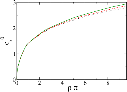
Figure 2: (Color online). Zero sound velocity $c_{s}^{0}$ vs. planar density $\rho$. Three values of the scaled interaction strength: $g=10^{-5}$ (dotted curve), $g=0.35$ (dashed curve), $g=0.6$ (solid curve). The zero sound velocity is in units of $a_{z}\omega_{z}$, density in units of $1/a_{z}^{2}$, and lengths in units of $a_{z}$.

Now we consider a density $\rho$ large enough so that some excited axial harmonic levels are populated. In this case, the velocity of zero sound is given by the zero of the determinant of the matrix in the l.h.s. of Eq. (27) with $\omega>Q$. The calculation is again straightforward and the results are reported in Fig. 2, where we display the zero sound velocity $c_{s}^{0}$ as a function of the planar density $\rho$. As it happens in the strictly 2D case, for a given value of the planar density $\rho$, $c_{s}^{0}$ increases by increasing the repulsive two body interaction $g$.

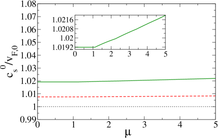
Figure 3: Ratio $c_{s}^{0}/v_{F,0}$ vs. chemical potential $\mu$. Three values of the scaled interaction strength: $g=0$ (dotted curve), $g=0.35$ (dashed curve), $g=0.6$ (solid curve). Note that the dotted curve is superimposed to the solid one. The velocities $c_{s}^{0}$ and $v_{F,0}$ are in units of $a_{z}\omega_{z}$, lengths in units of $a_{z}$, and the chemical potential in units of $\hbar\omega_{z}$.

In Fig. 3 we plot the quantity $c_{s}^{0}/v_{F,0}$ as a function of the chemical potential $\mu$. When $g=0$ one finds that $c_{s}^{0}$=$v_{F,0}$. If $g>0$ but $\mu$ is sufficiently small so that only the lowest axial mode is populated, then the quantity $c_{s}^{0}/v_{F,0}$ does not change when the chemical potential is varied (dashed line). This behavior corresponds to the one described by Eq. (33). When the chemical potential is greater than a critical value $\mu_{c}$, excited axial modes begin to be occupied by the fermions and $c_{s}^{0}/v_{F,0}$ grows with $\mu$ (see the inset of Fig. 3).

IV First sound

In this section we analyze the collisional case of a normal paramagnetic Fermi gas. To analyze a sound wave that travels in a planar direction it is important to determine the collision time $\tau$ of the gas. According to bruun and gupta , if the local Fermi surface is not strongly deformed then $\tau=\tau_{0}(T/T_{F})^{2}$, where $\tau_{0}=1/(\rho^{(3D)}\sigma v_{F})$ with $\sigma$ the scattering cross-section and $\rho^{(3D)}$ the 3D density. Instead, if the local Fermi surface is strongly deformed, as in our case, then the collision time is simply given by $\tau=\tau_{0}$ gupta . It is easy to find that in our 2D geometry $\tau_{0}\sim 1/(\omega_{z}\rho a_{F}^{2})$. Setting $\omega$ the frequency of oscillation of the sound wave, the wave propagates in the collisionless regime if $\omega\tau\gg 1$ and in the collisional regime if $\omega\tau\ll 1$.

In the collisional regime by adopting the equations of hydrodynamics landau ; fetter ; negele the planar first sound velocity $c_{s}$ of the Fermi gas is given by the zero-temperature formula

$$c_{s}=\sqrt{{\rho\over m}{\partial\mu\over\partial\rho}}\;.$$ (37)

By using this formula and Eq. (18) we determine the behavior of $c_{s}$ versus $\rho$ and of $c_{s}/v_{F,0}$ as a function of $\mu$, as shown in Fig. 4 and in Fig. 5, respectively. These figures, obtained both for $g=0$ and for $g>0$ display shell effects, namely jumps of the first sound velocity $c_{s}$ when the atomic fermions occupy a new axial harmonic mode.

If the interaction is negligible in the equation of state, the values $\rho_{c}$ of the density at which such jumps occur may be analytically obtained from Eq. (18). In fact, we obtain the behavior of the planar density as a function of the chemical potential by setting $g=0$ in the Eq. (18) and performing the sum over the quantum number $j$. Then, we get

$$\rho=\sum_{j=0}^{I[{\mu\over\hbar\omega_{z}}]}{1\over\pi a_{z}^{2}}\,\left({\mu\over\hbar\omega_{z}}-j\right)={1\over\pi a_{z}^{2}}\,S({\mu\over\hbar\omega_{z}})\;,$$ (38)

where

$$S(x)=(1+I[x])(x-{1\over 2}I[x])\;$$ (39)

with $I[x]$ the integer part of $x$. Eq. (38) with Eq. (39) represents a simple analytical formula which gives the uniform planar density $\rho$ of the Fermi gas as a function of the chemical potential $\mu$. The values $\rho_{c}$ signing the jumps can be obtained from Eq. (38) with with Eq. (39). The jumps of the first sound velocity are given by

$$\rho_{c}=\displaystyle{\frac{k(k+1)}{2\pi a_{z}^{2}}}\quad\mbox{with}\quad k=1,2,3,...\;.$$ (40)

When the critical value of the density is approached from the left, from Eq. (37) we find that the sound velocity is

$$c_{s}^{-}=\displaystyle{\omega_{z}a_{z}\sqrt{\frac{k+1}{2}}}\;,$$ (41)

while when $n_{c}$ is approached form the right, we find

$$c_{s}^{+}=\displaystyle{\omega_{z}a_{z}\sqrt{\frac{k}{2}}}\;.$$ (42)

The height of the first jump of $c_{s}$ is then given by

$$\Delta c_{s}=\omega_{z}a_{z}\frac{\sqrt{k+1}-\sqrt{k}}{\sqrt{2}}\;.$$ (43)

When interactions are not negligible in the equation of state, one must use Eq. (18) to get the values of $\rho$ for which the slope of $\mu$ exhibits discontinuities, and calculate the corresponding discontinuities in $c_{s}$. For example, at the first discontinuity, which appears when $l_{max}$ goes from $0$ to $1$ the value of the density is

$$\rho_{c}=\frac{1}{\pi a_{z}^{2}}\frac{1}{1+gu_{0,0}}=\frac{1}{\pi a_{z}^{2}}\frac{1}{1+F_{0}}\;.$$ (44)

The corresponding discontinuity exhibited by the first sound velocity is

$$\Delta c_{s}=c_{s}^{-}-c_{s}^{+}\;,$$ (45)

where

$$c_{s}^{-}=\omega_{z}a_{z}\sqrt{\frac{1}{(1+gu_{0,0})[1+g(u_{0,0}-u_{1,1})]}}\;,$$ (46)

and

$$c_{s}^{+} = \omega_{z}a_{z}$$

$$\sqrt{\frac{1+g[u_{0,0}+u_{1,1}+g(u_{0,0}u_{1,1}-{u^{2}}_{0,1})]}{[1+g(u_{0,0}-u_{1,1})][2+g(u_{0,0}-2u_{0,1}+u_{1,1})]}}\;,$$

where the $u$’s are given in Tab. 1. We observe that these shell effects are similar to the ones occurring in the 1D-3D crossover sala-reduce1 , where the jumps are sharper because the sound velocity goes to zero in correspondence of the filling of planar harmonic modes, showing the crucial role played by the dimensionality. In the next section we shall discuss the experimental conditions necessary to observe shell effects in the velocity of first sound.

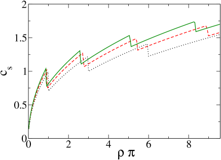
Figure 4: (Color online). First sound velocity $c_{s}$ as a function of the transverse density $\rho$. Three values of the scaled interaction strength: $g=0$ (dotted curve), $g=0.35$ (dashed curve), $g=0.6$ (solid curve). The first sound velocity is in units of $a_{z}\omega_{z}$, density in units of $1/a_{z}^{2}$, and lengths in units of $a_{z}$.

Now we comment on the 2D-3D crossover in our fermionic gas, starting from the strictly 2D case, corresponding to $l_{max}=0$ in Eq. (16). In this case the chemical potential $\mu$ is given by Eq. (35) and therefore from Eqs. (31) and (37) one finds

$$c_{s}={v_{F,0}\over\sqrt{2}}\sqrt{(1+gu_{0,0})}\;,$$ (48)

or, in terms of the Landau parameter $F_{0}$

$$c_{s}=\frac{\sqrt{\frac{2}{m}(\mu-\pi\hbar\omega_{z}a_{z}^{2}\rho F_{0})}}{\sqrt{2}}\sqrt{1+F_{0}}\;$$ (49)

recovering the usual result for a 2D Fermi system. Such a behavior is illustrated by the first plateau in Fig. 5. Incidentally, note that when $F_{0}\simeq 0$ the zero sound velocity (36) is larger than the first sound velocity (49) by a factor of $\sqrt{2}$. In our case, the quantity $F_{0}$ is smaller than one. Then the two velocities are different between each other also when $F_{0}$ remains finite.

We observe that the first sound velocity depends explictly on the chemical potential. In fact, remembering the relation between $\mu$ and $\rho$ given by Eq. (18), and using Eqs. (38) and (39), one may show that the velocity of first sound takes the form:

$$c_{s}=\sqrt{2\mu\over m}\sqrt{{1\over 2}\Big{[}1-{1\over 2}\frac{I[\mu/\hbar\omega_{z}]}{\mu/\hbar\omega_{z}}+\frac{t(g)}{\mu/\hbar\omega_{z}}\Big{]}}\;,$$ (50)

where $t(g)$ is a complicated but analytical function of $g$ and of the matrix elements $u$’s, which vanishes if $g=0$. We stress that the chemical potential $\mu$ depends on the planar density $\rho$ and on the interaction strength $g$. Fig. 5 shows how $c_{s}/v_{F,0}$ explictly depends on $\mu$ when axial harmonic states other than the ground states are occupied. From Eq. (50) one finds that for any $g$ at very large $\rho$ (i.e. also very large $\mu$) the speed of sound is given by:

$$c_{s}={1\over 2}\sqrt{2\mu\over m}\;.$$ (51)

In absence of two-body interactions ($g=0$) for $\rho>{1/(\pi a_{z}^{2})}$, i.e. for $\mu>\hbar\omega_{z}$, several single-particle states of the axial harmonic well are occupied and the gas exhibits the 2D-3D crossover. Finally, for $\rho\gg{1/(\pi a_{z}^{2})}$, i.e. for $\mu\gg\hbar\omega_{z}$, the Fermi gas becomes 3D. In this case from Eqs. (37), (38) and (39) one finds

$$\mu=(2\pi)^{1/2}\,\hbar\omega_{z}\,(a_{z}^{2}\rho)^{1/2}\;,$$ (52)

$$c_{s}=\sqrt{2}\ (2\pi)^{1/4}\,a_{z}\omega_{z}\,(a_{z}^{2}\rho)^{1/4}\;.$$ (53)

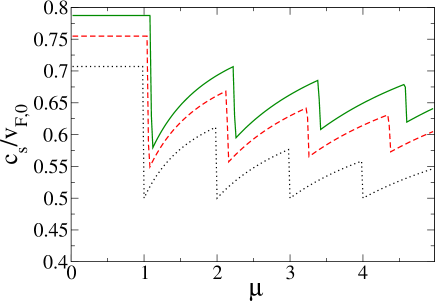
Figure 5: (Color online). The ratio $c_{s}/v_{F,0}$ versus chemical potential $\mu$. Chemical potential is in units of $\hbar\omega_{z}$. We report behavior for $g=0$ (dotted curve), $g=0.35$ (dashed curve), $g=0.6$ (solid curve). The velocities $c_{s}$ and $v_{F,0}$ are in units of $a_{z}\omega_{z}$, lengths in units of $a_{z}$, and the chemical potential in units of $\hbar\omega_{z}$.

We observe that starting from the familiar Thomas-Fermi formula for the 3D local density $\rho(z)$ of the Fermi gas under axial harmonic confinement, given by

$$\rho(z)={(2m)^{3/2}\over 3\pi^{2}\hbar^{3}}\left(\mu-{1\over 2}m\omega_{z}^{2}\,z^{2}\right)^{3/2}\;,$$ (54)

and integrating over $z$, one obtains exactly Eq. (52).

V Experimental feasibility

We now discuss the experimental conditions to detect the zero and first sound in a quasi-2D two-component Fermi gas. We suppose that in the $(x,y)$ plane the system is in a square box of length $L=20$ $\mu$m, while in the axial direction $z$ there is a harmonic confinement characterized by a frequency of $160$ kHz, which corresponds to a characteristic length $a_{z}\simeq 0.1$ $\mu$m. We consider ⁴⁰K atoms trapped in the two hyperfine states $|f=9/2,m_{f}=7/2\rangle$ and $|f=9/2,m_{f}=-7/2\rangle$ with $f$ the total atomic spin and $m_{f}$ its axial projection. In this case the $s$-wave scattering length reads $a_{F}=174$ $a_{0}$, where $a_{0}=0.53\cdot 10^{-10}$ m is the Bohr radius regal . For this value of $a_{F}$, we can determine the value of the collective mode frequency $\omega_{c}$ which discriminates between the collisionless and the hydrodynamic regimes. In fact, the collision time $\tau$ can be estimated as $\tau\sim 1/(\omega_{z}\rho a_{F}^{2})$ and the corresponding critical frequency is $\omega_{c}=2\pi/\tau\sim\omega_{z}(2\pi\rho a_{F}^{2})$. If the frequency $\omega$ of the collective mode is much greater than $\omega_{c}$ (i.e. for $\omega\gg\omega_{c}$) the system is in the collisionless regime; otherwise (i.e. for $\omega\ll\omega_{c}$) the collective excitation is hydrodynamic-like.

One can experimentally change $\omega_{c}$ in the Fermi gas of ⁴⁰K atoms by varying the planar density $\rho$. For instance, from Fig. 4 and Eq. (39) one finds that in correspondence to $(\rho a_{z}^{2})\pi=1/2$ the system is strictly 2D. In this case, the planar density is $\rho\simeq 1.6\cdot 10^{13}$ atoms/$m^{2}$, the total number of atoms is $N=\rho L^{2}\simeq 6.4\cdot 10^{3}$, and the critical frequency reads $\omega_{c}\simeq 1.4$ kHz. In addition, the zero sound velocity is $c_{s}^{0}=v_{F,0}\simeq 0.02$ m/s, while the first sound velocity is $c_{s}=v_{F,0}/\sqrt{2}\simeq 0.014$ m/s. Moreover, one finds that the scaled interaction strength is $g=2a_{F}/a_{z}\simeq 0.18$. To conclude, we observe that one can change the critical frequency $\omega_{c}$ also by varying the scattering length $a_{F}$ via magnetic Feshbach resonances.

VI Conclusions

In the present paper we have considered a dilute and ultracold interacting disk-shaped Fermi gas confined in the axial direction by a strong harmonic trap and uniform in the two planar directions. In particular, we have analyzed the behavior of the velocity of propagation of the zero and first sound modes in this gas.

In the first part of the paper, we have studied the zero sound mode from the density-density response function within the linear response theory and under the random phase approximation. We have obtained the zero-sound dispersion law by calculating the poles of the density-density response function. Then we have analyzed the behavior of the velocity of the zero sound as a function of the planar density for different values of the Fermi-Fermi scattering length. We have verified that as in the strictly two dimensional case, in correspondence of a given value of the planar density, the zero sound velocity increases as a consequence of the increasing of the strength of the fermion-fermion interaction. We have studied, moreover, the behavior of the ratio between the zero sound velocity $c_{s}^{0}$ and the planar Fermi velocity $v_{F,0}$ at varying of the chemical potential; when, in presence of a non vanishing fermion-fermion interaction, the chemical potential is greater than a critical value, excited axial modes begin to be occupied by the fermions and $c_{s}^{0}/v_{F,0}$ grows with $\mu$. In principle, the same kind of analysis may be carried out in presence of a harmonic potential in the transverse radial plane instead of the axial direction (see sala-reduce1 ). In this case, the treatment of the problem becomes much more complicated. In fact, the cigar-shaped configuration is characterized by two quantun mumbers related to the harmonic energetic levels in the planar directions. However, we expect for the zero sound velocity the same behavior as in the case of the only axial harmonic trapping.

In the second part of the paper, from the formula which relates the chemical potential of a disk-shaped Fermi gas to its uniform planar density, we have calculated the collisional sound velocity of the system. We have found that this sound velocity gives a clear signature of the dimensional crossover of the two-component Fermi gas. Our calculations suggest that the dimensional crossover induces shell effects, which can be experimentally detected. In fact, as in 1D-3D crossover sala-reduce1 , also in the 2D-3D crossover the sound velocity exhibits jumps in correspondence of the filling of axial harmonic modes. We have investigated the behavior of the ratio between the first sound velocity $c_{s}$ and the planar Fermi velocity as a function of the chemical potential. We stress that our study shows that when only the ground state of the harmonic well is populated and when the chemical potential is sufficiently large so many excited axial modes are occupied, our results reproduce the behavior of a 2D and a 3D Fermi system, respectively.

Finally, we have discussed the possibility of observing in experiments the zero and first sound by using gases of ⁴⁰K atoms trapped in the two lowest hyperfine states. In particular, we have estimated the sound-mode frequency which discriminates between the collisionless and hydrodynamic regime. We have found that these regimes require severe geometric and thermodynamical constraints, but they can be reached with the available experimental setups.

This work has been partially supported by Fondazione CARIPARO. The authors thank Giovanni Modugno for useful suggestions.

References

- (1) C.J. Pethick and H. Smith, Bose-Einstein Condensation in Dilute Gases (Cambridge Univ. Press, Cambridge, 2002).
- (2) L.P. Pitaevskii and S. Stringari, Bose–Einstein Condensation (Oxford Univ. Press, Oxford, 2003).
- (3) B. DeMarco and D.S. Jin, Science 285, 1703 (1999).
- (4) A.G. Truscott, K. E. Strecker, W. I. McAlexander, G. B. Partridge and R. G. Hulet, Science 291, 2570 (2001).
- (5) G. Modugno, G. Roati, F. Riboli, F. Ferlaino, R. J. Brecha, M. Inguscio , Science 297, 2240 (2002).
- (6) M. Greiner, C.A. Regal, and D.S. Jin, Nature 426, 537 (2003).
- (7) S. Jochim, M. Bartenstein, A. Altmeyer, G. Hendl, S. Riedl, C. Chin, J. Hecker Denschlag, R. Grimm, Science 302, 2101 (2003).
- (8) A. Gorlitz, J. M. Vogels, A. E. Leanhardt, C. Raman, T. L. Gustavson, J. R. Abo-Shaeer, A. P. Chikkatur, S. Gupta, S. Inouye, T. Rosenband, and W. Ketterle Phys. Rev. Lett. 87, 130402 (2001).
- (9) F. Schreck, L. Khaykovich, K. L. Corwin, G. Ferrari, T. Bourdel, J. Cubizolles, and C. Salomon Phys. Rev. Lett. 87, 080403 (2001).
- (10) T. Kinoshita, T. Wenger, and D. S. Weiss, Science 305, 1125 (2004).
- (11) J. Schneider and H. Wallis, Phys. Rev. A 57, 1253 (1998).
- (12) L. Salasnich, J. Math. Phys. 41, 8016 (2000).
- (13) L. Salasnich, B. Pozzi, A. Parola, L. Reatto, J. Phys. B 33, 3943 (2000); L. Salasnich, L. Reatto and A. Parola, in ’Perspectives in Theoretical Nuclear Physics VIII’, Ed. by G. Pisent et al, pp. 239-246 (World Scientific, Singapore, 2001).
- (14) P. Vignolo and A. Minguzzi, Phys. Rev. A 67, 053601 (2003).
- (15) G.M. Bruun and C.W. Clark, Phys. Rev. Lett. 83, 5415 (1999).
- (16) A. Minguzzi, P. Vignolo, M.L. Chiofalo, and M.P. Tosi, Phys. Rev. A 64, 033605 (2001).
- (17) K.K. Das, Phys. Rev. Lett. 90, 170403 (2003).
- (18) L. Salasnich, S.K. Adhikari, and F. Toigo Phys. Rev. A 75, 023616 (2007).
- (19) P. Capuzzi, P. Vignolo, F. Federici and M.P. Tosi, J. Phys. B: At. Mol. Opt. Phys. 37, S91 (2004).
- (20) T.K. Ghosh and K. Machida, Phys. Rev. A 73, 013613 (2006).
- (21) P. Capuzzi, P. Vignolo, F. Federici and M.P. Tosi, Phys. Rev. A 73, 021603(R) (2006).
- (22) P. Capuzzi, P. Vignolo, F. Federici and M.P. Tosi, Phys. Rev. A 74, 057601 (2006).
- (23) L. Landau and L. Lifshitz, Course in Theoretical Physics, Vol. 9, Statistical Physics (Pergamon, New York, 1959).
- (24) D. Pines and P. Noziers, The Theory of Quantum Liquids, Vol I, Normal Fermi Liquids (W.A. Benjamin, New York, 1966).
- (25) A.L. Fetter and J.D. Walecka, Quantum Theory of Many-Particle Systems (McGraw-Hill, Boston, 1971).
- (26) L. Salasnich and F. Toigo, J. Low. Temp. Phys. 150, 643 (2008).
- (27) J.W. Negele and H. Orland, Quantum Many Particle Systems (Westview Press, Boulder, 1998).
- (28) G.F. Giuliani and G. Vignale, Quantum Theory of the Electron Liquid (Cambridge University Press, 2005).
- (29) E. Lipparini, Modern Many Particle Physics (World Scientific, 2003).
- (30) L. Salasnich, A. Parola, and L. Reatto, Phys. Rev. A 69, 045601 (2004).
- (31) L. Salasnich, A. Parola, and L. Reatto, Phys. Rev. A 70, 013606 (2004).
- (32) E.Zaremba, Phys. Rev. A 57, 518 (1998).
- (33) J. Joseph, B. Clancy, L. Luo, J. Kinast, A. Turlapov, and J. E. Thomas, Phys. Rev. Lett. 98, 170401 (2007).
- (34) S. Gupta, Z. Hadzibabic, J.R. Anglin, and W. Ketterle, Phys. Rev. Lett. 92, 100401 (2004).
- (35) C.A. Regal and D.S. Jin, Phys. Rev. Lett. 90, 230404 (2003).