QPOs from Random X-ray Bursts around Rotating Black Holes

Abstract

We continue our earlier studies of quasi-periodic oscillations (QPOs) in the power spectra of accreting, rapidly-rotating black holes that originate from the geometric “light echoes” of X-ray flares occurring within the black hole ergosphere. Our present work extends our previous treatment to three-dimensional photon emission and orbits to allow for arbitrary latitudes in the positions of the distant observers and the X-ray sources in place of the mainly equatorial positions and photon orbits of the earlier consideration. Following the trajectories of a large number of photons we calculate the response functions of a given geometry and use them to produce model light curves which we subsequently analyze to compute their power spectra and autocorrelation functions. In the case of an optically-thin environment, relevant to advection-dominated accretion flows, we consistently find QPOs at frequencies of order of $\sim$ kHz for stellar-mass black hole candidates while order of $\sim$ mHz for typical active galactic nuclei ($\sim 10^{7}M_{\odot}$) for a wide range of viewing angles ($30^{{}^{\circ}}$ to $80^{{}^{\circ}}$) from X-ray sources predominantly concentrated toward the equator within the ergosphere. As in our previous treatment, here too, the QPO signal is produced by the frame-dragging of the photons by the rapidly-rotating black hole, which results in photon “bunches” separated by constant time-lags, the result of multiple photon orbits around the hole. Our model predicts for various source/observer configurations the robust presence of a new class of QPOs, which is inevitably generic to curved spacetime structure in rotating black hole systems.

1 Introduction

One of the more interesting findings of the X-ray timing analyses of the light curves of accreting compact objects in the past two decades has been the discovery of quasi-periodic oscillations (QPOs). These are broad features in the power spectra of these sources that range up to kHz frequencies in neutron star low-mass X-ray binaries (see, e.g., van der Klis 2000) and up to tens and even hundreds of Hz in accreting black hole binary systems (see, e.g., Cui et al. 1998 and Strohmayer 2001a, b), including QPO pairs with 2:3 frequency commensurability in the power spectra of certain black hole candidates (e.g. XTE J1550-564 and GRO J1655-40). Besides galactic binary sources, the presence of QPOs has also been reported in at least one ultra-luminous X-ray sources (ULX), namely NGC 5408 X-1 (see Strohmayer et al., 2007) at $\nu\sim 20$ mHz; in the context of active galactic nuclei (AGNs) Gierliński et al. (2008) recently discovered a $\sim 1$ hour X-ray periodicity in the narrow-line Seyfert 1 (NLS1) RE J1034+396, in which the periodicity is apparent in its light curve in distinction with those of the galactic binary black hole systems mentioned above that do not exhibit any such behavior.

The nature of QPO phenomenon in accreting black hole systems is at present largely unknown; it is also possible that this phenomenon is not the manifestation of a unique process, but that the observed diversity of QPO frequencies and sites may be due to a multitude of processes specific to the particular frequency and site. For the case of QPOs associated with black hole systems, the absence of an underlying, rotating solid surface object, implies that plausible explanations involve by necessity processes associated with the surrounding accretion disks. These include, among others, accretion disk precession due to the frame-dragging effects of a rapidly-rotating black hole (e.g. Cui et al., 1998; Merloni et al., 1999; Schnittman et al., 2006) (also see, e.g., Stella & Vietri 1998, for the same effect invoked to account for the kHz QPOs of Low Mass X-ray Binaries), accretion disk oscillatory modes (e.g. Nowak et al., 1997; Abramowicz & Kluźniak, 2001; Kato, 2001; Donmez, 2007, for diskoseismology), or the distribution of X-ray emitting “blobs” spanning a limited range around some specific radius of the Keplerian disk surrounding the black hole (e.g. Karas, 1999). There have also been studies of the correlations of the QPO frequencies with the properties of the associated X-ray spectra (e.g. Titarchuk & Fiorito, 2004).

An altogether different notion to QPO origin has been put forward recently by Fukumura & Kazanas (2008, hereafter FK08). These authors proposed that high frequency QPO (HFQPO) could be produced as a consequence of light echoes of X-ray flares occurring within the ergosphere of a Kerr black hole; they showed that due to frame-dragging of individual flare photons, a finite number of them reach far away observers after an integer number of additional orbits around the black hole to produce a geometry-induced “light echo” of the original flare (see, also, Meyer et al., 2006; Bursa et al., 2007, for a similar discussion). Studying two-dimensional (2D) near-equatorial photon propagation in a fully general relativistic calculation, FK08 showed that dragging of inertial frames leads approximately $15\%$ of the photons to a specific direction at infinity (an observer) after a time lag of $\Delta t\simeq 14\,M$ (where $M$ is black hole mass), independent of the relative position between the observer and the photon source. The independence of the lag on the relative phase between the observer and the source then guarantees a second peak in the Autocorrelation Function (ACF) at lag $\tau\simeq 14M$, which according to Fourier analysis, results in a prominent HFQPO signal at a frequency $\nu_{\rm QPO}\simeq 1/\Delta t\simeq 1.4\,(10M_{\odot}/M)$ kHz (where $M_{\odot}$ is the solar mass), even for a light curve that consists of flares randomly distributed within the ergosphere. Since the closest an accretion disk can approach the black hole is the radius of Innermost Stable Circular Orbit (ISCO), this effect is possible only when the ISCO lies within the black hole ergosphere, a condition that limits this effect to black holes with dimensionless spin parameter $a/M\mathrel{\raise 2.15277pt\hbox{$>$}\mkern-14.0mu\lower 2.58334pt\hbox{$\sim$}}0.94$.

The study of FK08 showed the prominent role of frame-dragging in producing lags independent of the relative source - observer position; as shown there, the absence of frame dragging for flares in a Schwarzschild geometry leads to lags which depend on the relative observer - source position and, for random flare positions, to absence of QPO features in the corresponding power spectra.

The original study of FK08 outlined the fundamental aspects behind this work, namely the importance of frame-dragging and the persistence of QPO presence, even for random positions of the X-ray flares within the ergosphere. However, it was restricted in its scope in that it was constrained to observers and sources near or on the black hole equatorial plane, i.e. $\theta_{s}\simeq\theta_{o}\simeq\pi/2$. Realistic constraints demand an enlarged study to include, at a minimum, observers at larger latitude positions, not least because it is expected that the column density of sources for lines of sight near the equator are sufficiently high to preclude propagation of photons without interaction with the surrounding matter; this could then lead either to their absorption or to their scattering and introduction of additional, random lags to their trajectories erasing the otherwise potential QPO signal. The goal of the present work is to remedy this deficiency by expanding the study of the corresponding lags to three-dimensional (3D) geometries allowing thus for arbitrary latitudes of both the observers as well as of the source of photons.

We would like to stress that the present models of “geometry-induced” QPOs (and also those of FK08) are not meant as an account of the so-called HFQPOs presented in the literature to date (e.g. Cui et al. 1998; Strohmayer 2001a, b). For one thing, the predicted QPO frequencies are $5-10$ times higher than the observed frequencies mentioned above (for the same black hole mass), and, for another, they do not produce their 2:3 frequency commensurability. Instead, the predicted QPOs should be viewed as an altogether new feature indicating the intrusion of an accreting gas within a black hole ergosphere, thereby providing an unequivocal evidence for the presence of rapidly rotating black holes.

Our paper is organized as follows: In §2 we provide a general description of our 3D QPO model, the details of the photon kinematics and response function of the system, and a prescription for constructing stochastic model light curves. In §3 we compute the autocorrelation functions (ACFs) and power spectral densities (PSDs) of the model light curves to show that they generally exhibit the QPO features as anticipated. Finally, in §4 we review our results, make contact with observations along with the limitations of our model, and conclude by discussing prospects of future work. Finally, in the Appendices we discuss the details the notion of locally isotropic emission in Kerr geometry and provide explicit functional forms relating the photon impact parameters to their local emission angles.

2 Model Details

The present treatment follows closely that of FK08, but generalizing the photon trajectories to 3D, thus allowing for positions of both the source and the observer at latitudes other than near equatorial. So, we consider photon emission in Kerr geometry of dimensionless angular momentum of a black hole $a$, described in Boyer-Lindquist coordinates $(r,\theta,\phi)$. As in FK08, here too we employ the usual geometrized units ($G=c=1$ where $G$ is the gravitational constant and $c$ is the speed of light) and normalize distance and time with the black hole mass $M$. For example, $1M$ corresponds to $1.5\times 10^{5}(M/M_{\odot})$ cm in distance and $5\times 10^{-6}(M/M_{\odot})$ sec in time. We consider the observer position at an arbitrary location ($r_{o},\theta_{o},\phi_{o}$), while correspondingly denoting the source coordinates as ($r_{s},\theta_{s},\phi_{s}$). This arrangement, therefore, allows for source locations not only at random azimuths but also at random polar angles. In thin accretion disks, the flares are likely confined to small latitudes, i.e. $\theta_{s}\simeq\pi/2$, but for quasi-spherical accreting flows such as advection-dominated accretion flows (ADAFs; e.g. Narayan & Yi, 1994), the overall source latitude can be much higher. As discussed in following subsections, in this last case, one can, in addition, weigh the emission at each latitude to fit one’s preferred flow model.

2.1 X-ray Flares

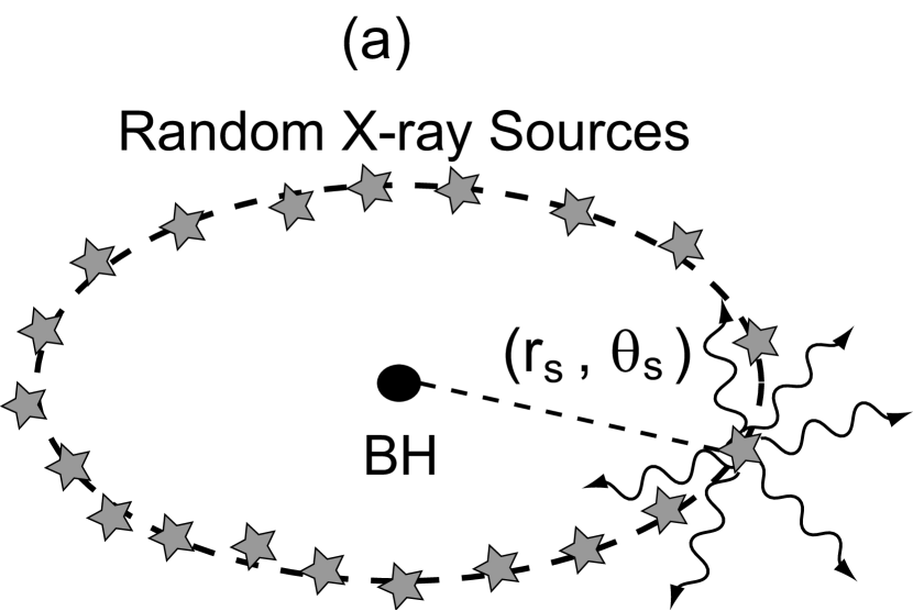
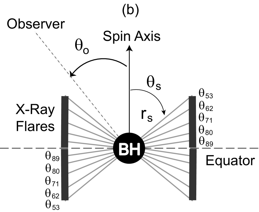
Figure 1: (a) Schematic view of the system considered in this paper. (b) Poloidal projection of the geometrical setup in this problem.

The X-ray emission of the sources we consider is regarded as the incoherent sum of a large number of instantaneous (i.e. short compared to the dynamical time) flares. We assume the typical duration of such a flare to be $\sim 1M$, presumably originating from local magnetic reconnections (e.g. Svensson & Zdziarski, 1994) or standing shocks in relativistic magnetized accretion (e.g. Takahashi et al., 2002; Fukumura et al., 2007). Concerning generation of X-ray flares within the ergosphere, Karas & Kopacek (2008) have attributed it to magnetic reconnection induced by frame-dragging, while Koide & Arai (2008) have considered magnetic reconnection within the ergosphere as a means of extracting energy from the black hole rotation. In general, these X-ray flares do not necessarily have to be confined exactly to the equatorial plane, and for this reason, in this work, we relax this restriction on the source vertical location. Therefore, in the specific cases that the emitting plasma is optically thin, the observed signal will contain contributions from sources in both upper and lower hemispheres.

It is important to mention that in this model both polar and azimuthal positions ($\theta_{s},\phi_{s}$) of each X-ray flash are randomly assumed (as long as they lie within or close to the ergosphere) while their cylindrical radius $r_{s}\sin\theta_{s}$ is fixed for simplicity to the radius of the ISCO of a Kerr hole with $a/M\simeq 0.99$, i.e. to $r_{s}\sin\theta_{s}\simeq 1.455M$. One of our primary interests is thus to probe the dependence on the source and the observer latitudes as illustrated in Figure 1b. To avoid the introduction of artificial coherent signals associated with orbital motion of these emitting sources, we also consider the flares to be randomly distributed in time in the following fashion: each X-ray burst occurs with a Poisson distribution of mean value equal to the Keplerian orbital timescale; $\Delta T\equiv T_{\rm orb}|\ln\{\textrm{rnd}(0,1)\}|$ where $T_{\rm orb}$ is the orbital time of the source at $(r_{s},\theta_{s})$ and rnd(0,1) is a random number between 0 and 1. We define that $T_{\rm orb}\equiv 2\pi\{(r_{s}\sin\theta_{s})^{3/2}+aM^{1/2}\}/M^{1/2}$.

The orbiting X-ray emitting plasma is assumed to be in Keplerian motion, either below or above an equatorial plane at $\theta_{s,i}$ where $i$ denotes the i-th source, i.e. rotating with the local Keplerian angular velocity (modified to take into account the black hole spin $a$)

$$\Omega_{s}=\left[\frac{M^{1/2}}{(r\sin\theta)^{3/2}+aM^{1/2}}\right]_{\rm source}\ ,$$ (1)

with all the quantities being evaluated at the source position. In the lab frame or the locally non-rotating reference frame (LNRF) each source has a total three-velocity of

$$v_{s} = \left[\frac{A\sin\theta}{\Sigma\Delta^{1/2}}(\Omega-\omega)\right]_{\rm source}\ ,$$ (2)

where we define $\Delta\equiv r^{2}-2Mr+a^{2}$, $\Sigma\equiv r^{2}+a^{2}\cos^{2}\theta$, $A\equiv(r^{2}+a^{2})^{2}-a^{2}\Delta\sin^{2}\theta$, and frame-dragging of the local inertial frame is denoted by $\omega\equiv 2Mra/A$. In the LNRF, as one can see, rotation of a local inertial frame $\omega$ has been subtracted by definition.

2.2 Null Geodesics

Neglecting external interactions between photons and particles, each null geodesic (i.e. photon orbit) is uniquely characterized by two constants of motion, $\xi$ and $\eta$, where $\xi$ is the axial component of angular momentum and $\eta$ closely related to its polar component (e.g. Bardeen et al., 1972; Chandrasekhar, 1983). For given $\eta$ and $\xi$, a photon orbit in Kerr geometry is generally governed by the following equations of motion (e.g. Bardeen et al., 1972; Chandrasekhar, 1983);

$$\dot{t} = \frac{(r^{2}+a^{2})\Xi+a\Delta\xi-a^{2}\Delta\sin^{2}\theta}{\Delta\Sigma}\ ,$$ (3)

$$\dot{r}^{2}\Sigma^{2} = \Xi^{2}-\Delta\{\eta+(\xi-a)^{2}\}\ ,$$ (4)

$$\dot{\theta}\Sigma^{2} = \eta+(a^{2}-\xi^{2}\csc^{2}\theta)\cos^{2}\theta\ ,$$ (5)

$$\dot{\phi} = \frac{a(2Mr-a\xi)+\xi\Delta\csc^{2}\theta}{\Delta\Sigma}\ ,$$ (6)

where $\Xi\equiv r^{2}+a^{2}-a\xi$ and an overdot denotes derivative with respect to the affine parameter. Note that equations (4) and (5) provide only the squares of $\dot{r}$ and $\dot{\theta}$. In order to avoid the issue of determination of appropriate signs for $\dot{r}$ and $\dot{\theta}$, for the actual numerical determination of the orbits we use instead the second derivatives of equations (4) and (5)

$$\ddot{r} = \frac{2r\dot{r}\Xi-\dot{r}\left(r-M\right)\left\{\eta+(\xi-a)^{2}\right\}-\Sigma\left\{2r\dot{r}-a^{2}\sin(2\theta)\dot{\theta}\right\}\dot{r}^{2}}{\dot{r}\Sigma^{2}}\ ,$$ (7)

$$\ddot{\theta} = \frac{\xi^{2}\cot\theta\csc^{2}\theta\dot{\theta}-a^{2}\sin(2\theta)\dot{\theta}/2-\Sigma\left\{2r\dot{r}-a^{2}\sin(2\theta)\dot{\theta}\right\}\dot{\theta}^{2}}{\dot{\theta}\Sigma^{2}}\ .$$ (8)

The initial conditions necessary for the integration of the orbit equations involve, besides the source position, ($r_{s},\theta_{s})$, also the two angles of photon directions and the values of $\dot{r}$ and $\dot{\theta}$; the last four quantities are not independent but they can be expressed in terms of ($r_{s},\theta_{s})$ and the values of the impact parameters $\eta$ and $\xi$ as discussed in §2.3.

2.3 Locally Isotropic Emission

In the absence of any information concerning the angular distribution of the photons emitted at a given flare, the most conservative assumption is that the emission is isotropic in the rotating fluid rest frame. However, the proximity of the X-ray sources to the black hole and the associated source motion ($v_{s}\simeq 0.6\,c$) and strong field geometry along with the fact that the coordinate system for the integration of the photon orbit equations is that of the LNRF, require that the notion of photon isotropy be transformed to this frame and that the impact of the Kerr metric on the notion of isotropy be considered with some care. Below we discuss our prescription of local isotropic emission, while more details can be found in Appendix A.

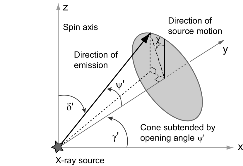
Figure 2: Geometry of local emission in the LNRF described in the text.

The geometry of photon emission is depicted in Figure 2. We assume the black hole spin axis to be in the z-direction while the local fluid velocity $v_{s}$ in the y-direction; $\psi$ is the angle between the emitted photon and the instantaneous direction of source motion (y-axis) in the fluid frame, while $\psi^{\prime}$ is the corresponding angle in the LNRF. For a given $\psi$ the precise direction of emission is determined by the angle $\chi$ confined in the plane orthogonal to the y-axis. The relation between $\psi$ and $\psi^{\prime}$ is then (the angle $\chi$ remains invariant)

$$\psi^{\prime}(\beta,\psi)=\cos^{-1}\left(\frac{\beta+\cos\psi}{1+\beta\cos\psi}\right)\ ,$$ (9)

where $\beta\equiv v_{s}/c$, while the differential solid angle and opening angle are transformed respectively as

$$d(\cos\psi^{\prime})=\frac{1-\beta^{2}}{(1+\beta\cos\psi)^{2}}\,d(\cos\psi)\ ,~{}~{}~{}~{}~{}~{}~{}~{}d\psi^{\prime}(\beta,\psi)=\frac{(1-\beta^{2})^{1/2}}{1+\beta\cos\psi}d\psi\ .$$ (10)

Isotropy in the fluid frame implies equal number of photons per unit solid angle $N_{0}$, i.e. $dN/d\Omega\equiv N_{0}$ over the entire sky in the fluid rest frame. However, when computing photon geodesics we choose incrementally not the solid angle but the angles $\psi$ and $\chi$. Then, the number of photons emitted per increment of the polar angle $\psi$ is $dN/d\psi=2\pi N_{0}\sin\psi$ and therefore the increment of the angle $\chi$ should be equal to $1/(2\pi N_{0}\sin\psi)$ so that each solid angle element at a given $\psi,\chi$ contains one photon.

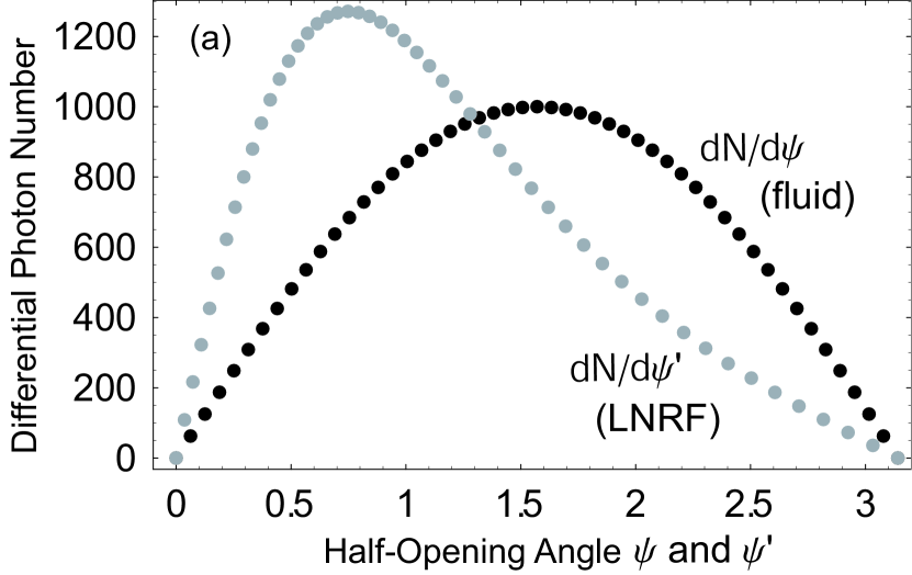
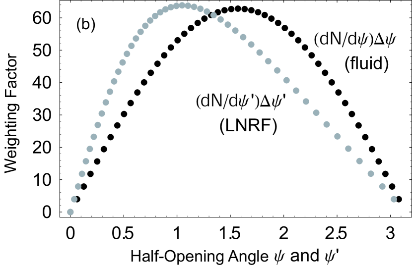
Figure 3: Comparison between the fluid rest-frame and the LNRF with $\beta=0.5$ for (a) Differential photon number distribution per emitting angle as a function of respective emitting angle in the fluid frame (dark) and the LNRF (gray). (b) Corresponding bin-corrected photon distribution (i.e. weighting factor) in the fluid frame (dark) and the LNRF (gray). We take $N_{0}=1000$ and $\Delta\psi=\pi/50$.

The Lorentz boost to the LNRF skews the photon distribution with angle resulting in larger number of photons being emitted along the direction of source motion with the distribution as a function of the polar angle $\psi$ (or $\psi^{\prime}$) given by the function

$$f(\beta,\psi^{\prime})\equiv\frac{(1-\beta^{2})\sin\psi^{\prime}}{(1-\beta\cos\psi^{\prime})^{2}}=\frac{(1+\beta\cos\psi)\sin\psi}{(1-\beta^{2})^{1/2}}\equiv f(\beta,\psi)\ .$$ (11)

In Figure 3a the photon distribution as a function of the polar angle $\psi$ for $\beta=0$ (dark dots for the fluid frame) and also as a function of $\psi^{\prime}$ for $\beta=0.5$ (gray dots for the LNRF) is shown. We take $N_{0}=1000$ and $\Delta\psi=\pi/50$. However, as indicated above in equation (10), the Lorentz boost transforms also the width of the the angular bin $\Delta\psi$; because of that, as shown in Appendix A, the number of photons per angular bin is invariant (as it should for photon number conservation), proportional to $\sin\psi\Delta\psi$. So each angular bin $\Delta\psi^{\prime}$ in the LNRF has the same number of photons as the corresponding bin $\Delta\psi$ in the fluid rest frame, but these photons are now received at a smaller angle $\psi^{\prime}$, given in terms of $\psi$ by equation (9). This distribution is shown in Figure 3b, where the number of photons per angular bin $f(\beta,\psi^{\prime})\Delta\psi^{\prime}=(dN/d\psi^{\prime})\Delta\psi^{\prime}=(dN/d\psi)\Delta\psi$ – for the same values of $N_{0}$ and $\Delta\psi$ as in Figure 3a – is shown as a function of the angle $\psi$ (dark dots for the fluid frame) and $\psi^{\prime}$ (gray dots for the LNRF). It is apparent that a given number of photons per bin is found at smaller angles in the LNRF rather than in the fluid rest frame.

For our photon orbit calculations we transform an equally spaced (discrete) set of angles $\psi_{i}$ in the source rest frame to the corresponding angles $\psi^{\prime}_{i}$ in the LNRF and release at each such bin a number of photons equal to $2\pi N_{0}\sin\psi_{i}$. These photons are then distributed each in a single of as many equal intervals in the $\chi$ angle. The next step involves expressing local emitting angles $\delta^{\prime}$ and $\gamma^{\prime}$ (both measured in the LNRF) used in the integration of the photon trajectories in terms of the angles $\psi^{\prime}$ and $\chi$. The relations between these sets of angles can be obtained from trigonometric relations of the geometry shown in Figure 2 as

$$\cos\psi^{\prime}=\sin\delta^{\prime}\,\sin\gamma^{\prime}\ ,~{}~{}~{}~{}~{}~{}\cos\delta^{\prime}=\sin\psi^{\prime}\cos\chi\ ,$$ (12)

where the first of these equations was obtained from a spherical triangle for the cosine of the angle $\psi^{\prime}$ while the second one from relations of the projection of the geometry of the same figure onto the plane perpendicular to the y-axis (i.e. in the shaded ellipse of the same figure).

The next step in the calculation takes into account the effects of the local geometry curvature in the definition of local isotropy (see Fukumura & Kazanas, 2007, as an example of this issue in the simpler case of the Schwarzschild geometry) by relating the angles $\delta^{\prime}$ and $\gamma^{\prime}$ to the photon four-velocity components. In the LNRF the photon’s local emitting polar and azimuthal angles ($\delta^{\prime},\gamma^{\prime}$) are related to the four-velocity components through the relations

$$v^{\hat{r}} = \frac{A^{1/2}}{\Delta}\frac{\dot{r}}{\dot{t}}=\sin\delta^{\prime}\cos\gamma^{\prime}\ ,$$ (13)

$$v^{\hat{\theta}} = \left(\frac{A}{\Delta}\right)^{1/2}\frac{\dot{\theta}}{\dot{t}}=\cos\delta^{\prime}\ ,$$ (14)

$$v^{\hat{\phi}} = \frac{A\sin\theta}{\Sigma\Delta^{1/2}}\left(\frac{\dot{\phi}}{\dot{t}}-\omega\right)=\sin\delta^{\prime}\sin\gamma^{\prime}\ ,$$ (15)

which lead to

$$\cos\delta^{\prime} = \left(\frac{A}{\Delta}\right)^{1/2}\frac{\dot{\theta}}{\dot{t}}\ ,$$ (16)

$$\cot\gamma^{\prime} = \frac{\Sigma}{A^{1/2}\Delta^{1/2}\sin\theta}\frac{\dot{r}}{\dot{\phi}-\omega\dot{t}}\ ,$$ (17)

evaluated at the emitting location ($r_{s},\theta_{s},0$). Using equations (3) through (6) we can eliminate $\dot{t}$, $\dot{r}$, $\dot{\theta}$ and $\dot{\phi}$ from the above equations (16) and (17) in favor of the two impact parameters $\eta$ and $\xi$. We are thus led to two relations that connect the photon emission angles ($\delta^{\prime},\gamma^{\prime}$) to the photon impact parameters $(\xi,\eta)$. In fact, one can invert these relations to obtain $(\xi,\eta)$ as a function of these angles, i.e. $\xi=\xi(\delta^{\prime},\gamma^{\prime})$ and $\eta=\eta(\delta^{\prime},\gamma^{\prime})$ as shown in Appendix B. This now completes the problem of the choice of the orbit parameters consistent with isotropic emission in the fluid frame: For a given set of equally spaced values of $\psi_{i}$ (locally isotropic source in the fluid rest frame) one can compute $\psi^{\prime}_{i}$ and also determine the number of photons to be emitted and values of the azimuthal angle bins $\chi_{i}$; these are then used to compute the angles $\delta^{\prime}$ and $\gamma^{\prime}$, and then the corresponding impact parameters $\eta$ and $\xi$ along with the initial values of $\dot{r}(\delta^{\prime},\gamma^{\prime})$ and $\dot{\theta}(\delta^{\prime},\gamma^{\prime})$ that are used in the integration of the photon orbit by equations (7) and (8).

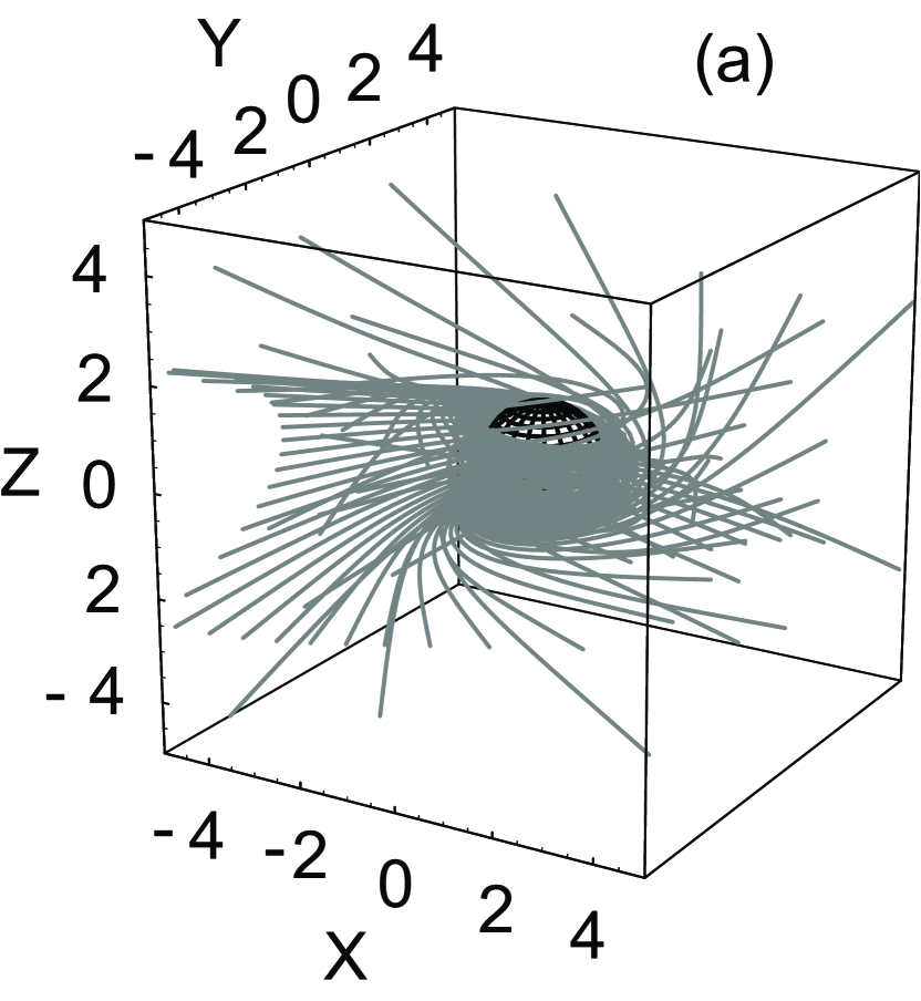
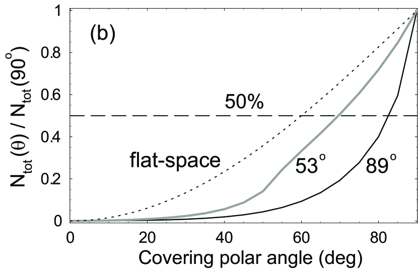
Figure 4: (a) Locally isotropic photon trajectories from a source at $(\sin\theta_{s},\phi_{s})=(89^{\circ},0^{\circ})$ for an opening angle of $\psi=80^{\circ}$ ($\psi^{\prime}=46^{\circ}$). We set $a/M=0.99$ and $N_{0}=100$. (b) Observed (cumulative) photon distribution $N_{\rm tot}(\theta)/N_{\rm tot}(90^{\circ})$ as a function of covering angle measured from the pole for various source geometries. It is normalized by the total photon number over $\pi/2$. We assume an equatorial source of $\theta_{s}=89^{\circ}$ (dark curve) and mid-latitude source of $53^{\circ}$ (gray curve), in comparison with stationary flat-space case (dotted curve).

An example of 3D photon trajectories from a locally isotropic emission is shown in Figure 4a where we consider emission with a half-opening angle of $\psi=80^{\circ}$ ($\psi^{\prime}=46^{\circ})$ from a source at $(\theta_{s},\phi_{s})=(89^{\circ},0^{\circ})$. Throughout this paper we assume $a/M=0.99$ as in Figure 4a, unless otherwise stated. Recall that our model considers now X-ray sources from both the upper and lower hemispheres with respect to the equator because of the optically-thin assumption of surrounding matter (see Fig. 1). Hence, the net observed emission will consist of a sum of these two components. We have confirmed that these photon trajectories are indeed almost symmetric with respect to the equator as expected. It should be noted, however, that for some particular emission angles this symmetry in trajectory with respect to the equator can be largely broken even for a small deviation of the source position from the equator. Due to the high velocity of the source ($\beta\sim 0.6$) for the values of $r_{s}$ and $a$ chosen, most of the emission is beamed forward in the direction of instantaneous source velocity. In fact we find that many backward-emitted photons (i.e. of $\psi>90^{\circ}$) subject to the Doppler and frame-dragging effects of the fast black hole rotation are forced to corotate in the hole direction (see FK08 for details in 2D cases). We also find that backward-emitted photons with $\psi\gtrsim 140^{\circ}$ end up crossing the the horizon, making no contribution to the observed signal. We should mention that the photon trajectories considered here also include many multiple orbits and higher-order photons; i.e. we also collect those photons that orbit around a black hole multiple times with some time-lags. The physical significance of these time-lags will be further discussed in §2.4.

To illustrate the effects of Doppler beaming and the black hole’s strong gravity for the considered source location ($r_{s}\sin\theta_{s}\simeq 1.45\,M$), we present in Figure 4b the cumulative, normalized distribution of photons $N_{\rm tot}(\theta)/N_{\rm tot}(90^{\circ})$ received by a distant observer at $r/M=100$, as a function of the observer’s inclination angle $\theta_{o}$. In the figure the solid dark curve corresponds to a nearly equatorial source ($\theta_{s}=89^{\circ}$), the gray curve to a source at the edge of the ergosphere ($\theta_{s}\simeq 53^{\circ}$) for the fixed cylindrical radius of the source, while the dotted curve to the flat-space distribution. It is apparent in this figure that photons emitted from equatorial position (in particular) are directed primarily at low latitude directions. While in flat-space 50% of the photons (horizontal dotted line) are emitted between angles $0^{\circ}-60^{\circ}$ as expected, in the equatorial source case of $\theta_{s}=89^{\circ}$ the half-way point has been extended to $\theta\simeq 82^{\circ}$. Similarly, while in flat-space polar angles $0^{\circ}-45^{\circ}$ include $\simeq 30\%$ of the entire photons emitted, in the present Kerr geometry they include roughly $10$ times less. This is an important issue related to the equivalent width of the (broad) fluorescence Fe lines whose red wing is presumably emitted by plasma closest to the ISCO of fast-rotating black holes with spin parameter similar to that used in producing our Figure 4b.

2.4 Response Functions and Light Curves

Following a methodology similar to that discussed in FK08, we first compute a source’s response function seen by a distant observer whose radial and azimuthal positions are set in this work to $(r_{o}/M,\phi_{o})=(100,0)$. This is a reasonable choice because at this distance the photon orbits are already nearly straight and thus their final (polar and azimuthal) directions are almost the same as those in flat spacetime. For a given source position at ($\theta_{s,i},\phi_{s,i}$) around a rapidly-rotating black hole we collect isotropically emitted photons (in the local rest-frame of an orbiting source) keeping track of its arrival time $t$ and final position ($\theta,\phi$) for each photon. As a result we can construct a response function seen by the observer $I_{i}(t,\theta_{o};\theta_{s,i},\phi_{s,i})$, which tells us photon counts as a function of photon’s arrival time from the i-th X-ray source at ($\theta_{s,i},\phi_{s,i}$). For an optically-thin environment we have contributions from sources at different source latitudes for the same source azimuth, however, for simplicity we assume that the sources closer to the equatorial plane are dominant, although it is found that this assumption does not make much difference to our final results shown §3 below.

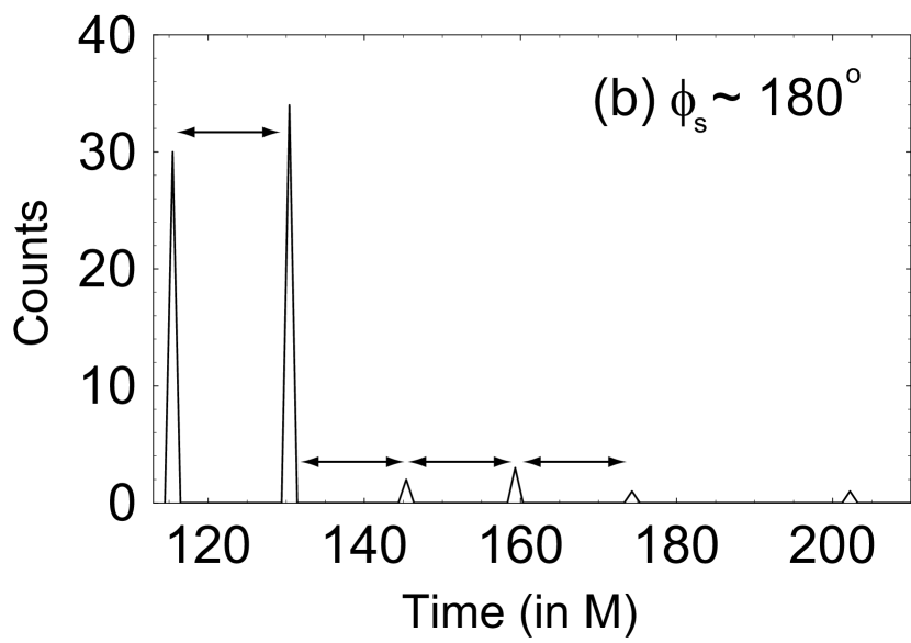
Figure 5: Synthetic response functions from a single X-ray source at $\theta_{s}=89^{\circ}$ with (a) $\phi_{s}\sim 4^{\circ}$ and (b) $\sim 180^{\circ}$ seen by an observer of $\theta_{o}=60^{\circ}$. Arrows indicate a constant lag of $\sim 14M$. Values of the other parameters are the same as in Figure 4.

The temporal resolution in the response function is taken to be $1M$ (corresponding to $5\times 10^{-5}$ sec for a $10M_{\odot}$ black hole), therefore the signal received by the observer is uniformly binned with this numerical accuracy. For computational purposes we approximate this signal, as precisely as possible, by a set of narrow Gaussians, also of width $1M$. Note the response function from each single source contains a characteristic temporal profile due to distinct photon trajectories between the source and the observer, and the profile also strongly depends on the observer’s polar position $\theta_{o}$ as well as the source position $(\theta_{s,i},\phi_{s,i})$. The observer’s collecting angle is chosen to be $\Delta\theta_{o}=\pm 1^{\circ}$. To produce a statistically significant outcome even for observer’s polar angles $\theta_{o}\mathrel{\raise 1.29167pt\hbox{$<$}\mkern-14.0mu\lower 2.58334pt\hbox{$\sim$}}30^{\circ}$ we consider a large number of sampling (a few $10^{6}$) per source. However, the common feature they share is found to be a constant time separation of $\simeq 14\,M$ between the major peaks of individual response functions, as found in FK08. To clearly illustrate these features of the response functions, we exhibit in Figure 5 the response functions from flares at (a) $\phi_{s}\sim 4^{\circ}$ and (b) $\sim 180^{\circ}$ for $\theta_{s}=89^{\circ}$ measured by an observer of $\theta_{o}=60^{\circ}$. A constant time lag of $\sim 14M$ (equivalent to $\sim 0.7$ msec for a $10M_{\odot}$) is clearly present. Due to multiple orbits around a fast-rotating black hole some photons make extra (integer-multiples) full orbits before reaching the observer.

The response functions are different in the precise positions of the major peaks, as one would expect, but, as argued above, the time-lag between the major peaks is roughly constant, $\Delta t\sim 14\,M$, regardless of the source location ($\theta_{s},\phi_{s}$). The reason for this behavior was discussed in detail in FK08 (it remains the same in the present case too): it is due to the frame-dragging effects which force all photons emitted at any relative position between source and the observer, to reach the latter only by “swinging” around the black hole; in following such trajectories, a non-negligible fraction ($\simeq 15-20\%$) of them reach the observer after multiple orbits around the black hole, inducing “light echoes” of nearly constant lag as shown in Figure 5. This is in agreement with similar relativistic calculations of broad iron line profiles by Beckwith & Done (2005) where they find that these higher-order photons contribute maximally $\sim 20-60$% of the total luminosity of the system. The persistent presence of such a constant time-lag in the response functions is the key factor leading to QPO features in the power spectra shown in §3. It should be noted that in the absence of strong frame-dragging (i.e. sources outside the ergosphere or Schwarzschild instead of Kerr black hole), the time interval among the peaks in the response functions is phase-dependent and precludes the presence of QPO in the power spectra for random source positions (see FK08).

As discussed in §2.1 the X-ray interval between flares $\Delta T$ is Poisson-distributed with mean value comparable to the Keplerian period at the ISCO. Therefore, the collective response function from the ensemble of X-ray flares (i.e. the bolometric light curve) is obtained by summing over every contribution from all the sources at $(\theta_{s,i},\phi_{s,i})$. That is,

$$I(t,\theta_{o})\equiv\sum_{i=1}^{n}I_{i}(t,\theta_{o};\theta_{s,i},\phi_{s,i})\ ,$$ (18)

where $n$ is a total number of random X-ray sources in our simulations. As an example, a synthetic light curve is shown in Figure 6a (i.e. superposition of all the response functions similar to Fig. 5) and its first $20M_{1}$ msec segment in Figure 6b where $M_{1}\equiv M/(10M_{\odot})$. In this specific case, the number of flares considered is $n=2000$ with the source positions confined to near the equatorial plane ($\theta_{s}=89^{\circ}$) while the observer is set at $\theta_{o}=60^{\circ}$. Because of the random positions ($\phi_{s,i}$) and bursting times of individual flares, the model light curve appears to be (in fact it is constructed to be) totally random with no apparent coherence (even in the absence of background noise). Nonetheless, the characteristic time-lag among the peaks in flux implicit in the form of the response function in Figure 5 is encoded in the light curve and it can be extracted (if present) by applying the standard time-series analysis techniques discussed in the next section §3.

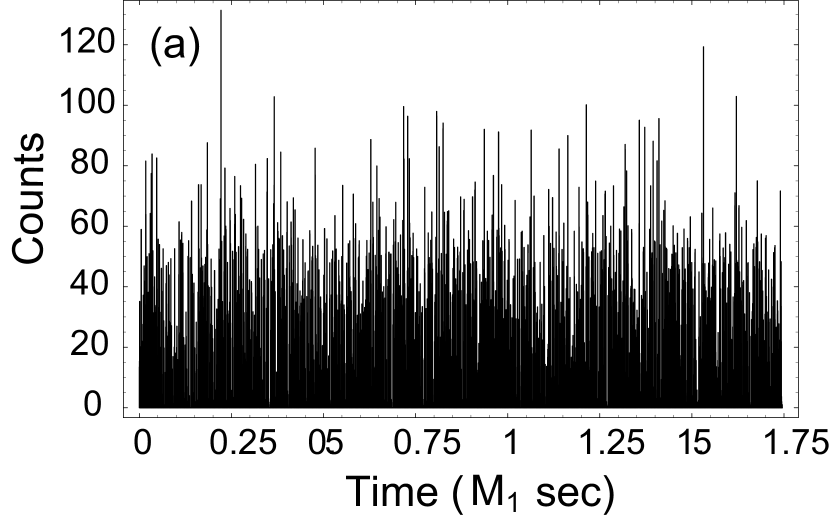
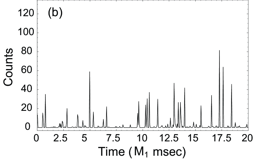
Figure 6: (a) Model light curves constructed from the synthetic response functions similar to those in Figure 5. We assume $n=2000$ random X-ray sources from $\theta_{s}=89^{\circ}$ for $\theta_{o}=60^{\circ}$. (b) The first $20M_{1}$ msec segment of (a). Values of the other parameters are the same as in Figure 4.

3 Power Spectra and Autocorrelation Functions

In this section we discuss in detail the timing analysis metrics, ACFs and PSDs, of the model light curves produced using the prescriptions discussed above, pertaining to rapidly-rotating black holes; more specifically we study the dependence of the ACFs and PSDs on the sources’ position and geometric structure as well as the position of the observer.

As shown in §2 above, the form of the response functions and hence of the model light curves we produce depend mainly on the sources’ latitudes (given that we average over their azimuths $\phi_{s,i}$). Because the effects of frame-dragging are most prominent for sources near the equator, we first examine cases where most of the X-ray emission is concentrated preferentially near the equatorial plane, i.e. of $\theta_{s,i}=89^{\circ}$ (and corresponding positions in the lower hemisphere). Regarding the observer’s inclination angle $\theta_{o}$ we consider a wide range from nearly face-on ($\theta_{o}\simeq 30^{\circ}$) positions to nearly edge-on ($\theta_{o}\simeq 85^{\circ}$) ones. Since our primary goal in this investigation is to generalize the previous 2D results of FK08, we restrict ourselves to a fast-rotating black hole case with $a/M=0.99$ for which the source X-ray photons are subject to strong dragging of inertial frame (i.e. inside the ergosphere). Note that for $a/M=0.99$ the ISCO radius is naturally well inside the ergosphere near the equatorial plane.

We also consider, for a given observer’s angle $\theta_{o}$, the dependence of the ACF and PSD on the latitudinal distribution of the sources within the ergosphere. To this end we compute also the response function for source positions at different vertical heights with $\Delta\theta_{s}=9^{\circ}$ by dividing the polar angle into five representative zones; i.e. $\theta_{s}=89^{\circ}$, $80^{\circ}$, $71^{\circ}$, $62^{\circ}$, and $53^{\circ}$ (see Fig. 1b). We then examine the effects of the sources’ vertical extent by computing light curves from sources with incrementally larger vertical extent, i.e. from sources whose emission consists of the sum of point sources at a number of heights corresponding to the following set of inclination angles: $\theta_{s}=\theta_{89^{\circ}}$ (i.e. equatorial sources), $\theta_{89^{\circ}+80^{\circ}}$, $\theta_{89^{\circ}+80^{\circ}+71^{\circ}}$, $\theta_{89^{\circ}+80^{\circ}+71^{\circ}+62^{\circ}}$, and $\theta_{89^{\circ}+80^{\circ}+71^{\circ}+62^{\circ}+53^{\circ}}$. We do not consider sources at heights that would correspond to angles smaller than $53^{\circ}$, because for the given value of black hole spin ($a/M=0.99$) and a vertical source whose equatorial foot point is at the ISCO, a larger height would place that section of the source outside the ergosphere, thereby producing no contribution to the QPO features via frame-dragging effect. Given that the effects of frame dragging decrease with increasing source height we expect the QPO effects to decrease with increasing vertical source extent.

The timing properties of the model light curves are explored for different relative positions between the source’s and observer’s polar angles by computing the ACF, $R(\tau;\theta_{o},\theta_{s})$, and the corresponding PSD, $P(\nu;\theta_{o},\theta_{s})$. For a discrete light curve $I(t_{o},\theta_{o};\theta_{s})$ the normalized ACF is given by

$$R(\tau_{j};\theta_{o},\theta_{s}) \equiv \sum_{k=1}^{L}\frac{I(t_{k},\theta_{o};\theta_{s})I(t_{k+j},\theta_{o};\theta_{s})}{I^{2}(t_{k},\theta_{o};\theta_{s})}\ ,$$ (19)

where $L$ is the number of time bins in the light curve of $I$. The corresponding PSD, in units of (rms/mean)²/Hz, is given by

$$P(\nu_{j};\theta_{o},\theta_{s}) \equiv \frac{2T}{N_{\rm ph}^{2}}|a_{j}|^{2}\ ,$$ (20)

where $T$ is the time duration of the light curve $I$ and $a_{j}$ is the Fourier amplitude defined by

$$I(t_{k},\theta_{o};\theta_{s})=\frac{1}{L}\sum_{j=1}^{L}a_{j}e^{2\pi ijk/L}\ ,$$ (21)

and $N_{\rm ph}$ is the total photon counts in the entire light curve of $I$. Also, $\tau_{j}$ and $\nu_{j}$ are timescale and frequency of a characteristic QPO signal, respectively.

3.1 Dependence on Viewing Angle

In this subsection we first present in Figure 7 a series of ACFs (left panels) and PSDs (right panels) as a function of the observer’s inclination (or viewing) angle $\theta_{\rm o}$ for model light curves from both near-equatorial sources, i.e. of $\theta_{s}=89^{\circ}$, and a source that is vertically extended in height, modeled as a sum of individual sources at heights that correspond to polar angles $\theta_{s}=89^{\circ}$, $80^{\circ}$, and $71^{\circ}$. These are shown in Figures 7a and b (equatorial source) and c and d (vertically extended source).

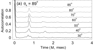
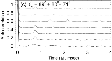
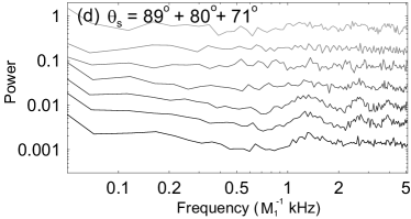
Figure 7: Autocorrelation functions (left panels) and power spectral densities (right panels) for various observer’s inclination angles where $\theta_{s}=\theta_{89^{\circ}}$ (upper panels) and $\theta_{s}=\theta_{89^{\circ}+80^{\circ}+71^{\circ}}$ (lower panels). We show $\theta_{o}=30^{\circ},40^{\circ},50^{\circ},60^{\circ},70^{\circ},80^{\circ},85^{\circ}$ from bottom to top curves with $\Delta\nu=0.6$ Hz bin size. Vertical positions of the curves are arbitrarily shifted for presentation purpose. Values of the other parameters are the same as in Figure 4.

As noted in FK08 the QPO signal in the light curves is imprinted by the frame dragging effects induced by the black hole spin. It is seen that a characteristic timescale of $\tau\sim 14M=0.73M_{1}$ msec is persistently present for a wide range of inclination $\theta_{o}$, which is a manifestation of the constant time-lag in the response function in Figure 5. Since these effects are more prominent for photon orbits that lie near the equator, this signature is more pronounced for arrangements that maximize the propagation of the received photons in this region. As shown in Figures 7a and b this effect is the most optimized for $\theta_{\rm o}\sim 50^{\circ}-60^{\circ}$; for observers at smaller inclination (polar) angles the effect is weaker because the influence of frame-dragging is much reduced for photons that propagate close to the black hole spin axis. This becomes apparent by the decrease of the ACF peak at $\tau\simeq 0.73M_{1}$ msec, or equivalently, the corresponding QPO amplitude with the decrease in $\theta_{\rm o}$ (Fig. 7a and b). The QPO amplitude decreases also for $\theta_{\rm o}>60^{\circ}$; the reason for that is the increase of the fraction of the poloidal plane orbits that connect the source and the observer; these photons do not orbit around the black hole with coherence and as such they do not contribute to the QPO amplitude but in fact they dilute it. That is, the total signal is the result of a superposition of a mixture of both coherent and incoherent signals.

Similarly, as shown in Figures 7c and d, a vertically extended source leads to reduction in the corresponding amplitudes of the ACF and QPO since the frame-dragging effects decrease as the source approaches the edge of the ergosphere. Comparison of Figures 7a and b with Figures 7c and d, which exhibit respectively the ACFs and PSDs for a set of observers at inclinations $\theta_{\rm o}=30^{\circ}$, $40^{\circ}$, $50^{\circ}$, $60^{\circ}$, $70^{\circ}$, $80^{\circ}$, $85^{\circ}$ for an equatorial (a,b) and a vertically extended source (c,d), confirms these notions; the QPOs are more prominent for sources confined near the equator than for those which are vertically extended. The former also persists over a wider range of values of $\theta_{o}$, being strongest for $\theta_{o}\sim 50^{\circ}-60^{\circ}$, while the latter, being intrinsically weaker, they disappear for $\theta_{o}\mathrel{\raise 2.15277pt\hbox{$>$}\mkern-14.0mu\lower 2.58334pt\hbox{$\sim$}}60^{\circ}$.

Finally, while the QPO and ACF secondary peak amplitudes do depend on the observer inclination, the corresponding QPO frequency and ACF peaks remain constant respectively equal to $\nu_{QPO}\sim 1.4M_{1}^{-1}$ kHz and $\tau\sim 0.73M_{1}$ msec, a value representing the length of the photon paths around the ISCO, becoming considerably wider only for $\theta_{\rm o}\mathrel{\raise 1.29167pt\hbox{$<$}\mkern-14.0mu\lower 2.58334pt\hbox{$\sim$}}30^{\circ}$.

3.2 Dependence on Source Concentration

If the X-ray sources originate from processes other than those associated with the surface of a thin disk (e.g. flaring events due to magnetic reconnection, polar shocks or wind/jets), then the source may not be exclusively distributed in an equatorial fashion. In this subsection we examine in greater depth the effects of extending the source dimension vertically on the ACFs and QPOs respectively. To this end we have produced the light curves starting with an equatorially concentrated source ($\theta_{s}=89^{\circ}$) and consider the light curves from more extended sources by incorporating into the light curve also photons from sources at larger heights, or smaller values of the angle $\theta_{s}$; this is done incrementally by considering additional sources of the same intensity at the following set of source polar angles: $\theta_{89^{\circ}+80^{\circ}}$, $\theta_{89^{\circ}+80^{\circ}+71^{\circ}}$, $\theta_{89^{\circ}+80^{\circ}+71^{\circ}+62^{\circ}}$, and $\theta_{89^{\circ}+80^{\circ}+71^{\circ}+62^{\circ}+53^{\circ}}$. We do not consider sources at any larger heights because for the conditions used here they would be outside the ergosphere and they would not contribute to the QPO signal by frame-dragging.

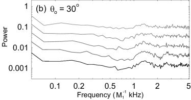
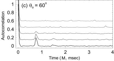
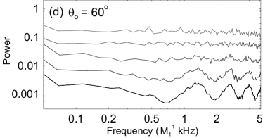
Figure 8: Autocorrelation functions (left panels) and power spectral densities (right panels) for various source distributions where $\theta_{o}=\theta_{30^{\circ}}$ (upper panels) and $\theta_{o}=\theta_{60^{\circ}}$ (lower panels). We show $\theta_{s}=\theta_{89^{\circ}}$, $\theta_{89^{\circ}+80^{\circ}}$, $\theta_{89^{\circ}+80^{\circ}+71^{\circ}}$, $\theta_{89^{\circ}+80^{\circ}+71^{\circ}+62^{\circ}}$, and $\theta_{89^{\circ}+80^{\circ}+71^{\circ}+62^{\circ}+53^{\circ}}$ from bottom to top curves with $\Delta\nu=0.6$ Hz bin size. Vertical positions of the curves are arbitrarily shifted for presentation purpose. Values of the other parameters are the same as in Figure 4.

In Figures 8a and b we present respectively the ACFs and PSDs for an observer at $\theta_{\rm 0}=30^{\circ}$ as the source height progressively increases to $\theta_{s}=53^{\circ}$ (i.e. sources extending all the way up to the static limit). Overall, the QPO signal does not appear to be very strong but it is present. We see that the additional (incoherent) photons dilute those with constant lag to cause the QPO to disappear with the source height. Similarly, in Figures 8c and d we present the ACFs and PSDs for an observer with high inclination of $\theta_{\rm o}=60^{\circ}$. We see that in this case the QPO becomes again prominent when the X-ray sources are distributed near the equator as the photons that reach these directions are under a strong influence of frame-dragging. It appears that the latitudinal extension of the sources up to $\theta_{s}\lesssim 71^{\circ}$ can yield a discernible QPO signature, although it is relatively weak.

4 Summary and Discussion

In the present work we have extended the earlier 2D treatment of FK08 to consider the 3D geometry of photon emission on the timing properties of accretion flows in the vicinity of rapidly spinning black holes. This has allowed us to explore the effects of placing both observers and sources at latitudes much different from the equatorial ones considered in FK08 and, using these results, to consider also photon sources which are extended, i.e. sources whose vertical dimension is comparable or larger than their radial one. Our results are fundamentally consistent with those of FK08: we find that for the same reasons discussed in FK08, here too, frame-dragging causes the photons to follow trajectories that by and large lead to a significant fraction of them reaching the observer after an additional orbit around the black hole; as such, for a single X-ray flare, an observer sees multiple bunches of photons that arrive with a constant time-lag of order of $\sim 14M$ (i.e. light echoes), independent of the source position relative to the observer. It is the independence of the lag on the source position that leads to the QPO in the signal of even a random ensemble of X-ray bursts, provided that they take place within the ergosphere. As elaborated in FK08, the resulting QPOs are different in character to those examined so far in the literature in that they do not require any modulation/oscillation as such in the signal. The difference in their character can be easily assessed in the data by calculating, in addition to the PSDs, also the ACFs, which in the present case has the form shown in Figures 7 and 8, i.e. a peak near zero (self-coherence) with a second one at $\tau\simeq 14M=0.73M_{1}$ msec (QPO), very different from that of an oscillatory form, corresponding to QPOs due to some oscillation in the X-ray flux (Fukumura, Dong, Kazanas, & Shrader, in preparation). In summary, for sources concentrated near the equator (e.g. $\theta_{s}\mathrel{\raise 1.29167pt\hbox{$<$}\mkern-14.0mu\lower 2.58334pt\hbox{$\sim$}}85^{\circ}$), we find the presence of persistent QPOs (and a series of harmonics) of $\nu_{QPO}\sim 1.4$ kHz for a $10M_{\odot}$ black hole (equivalently $\sim 1.4$ mHz for a $10^{7}M_{\odot}$ AGN) for a wide range of line-of-sight viewing angles (from $\sim 30^{\circ}$ to $\sim 80^{\circ}$). This QPO signal is the direct consequence of photon trajectories undergoing multiple rotations around the black hole due to its strong frame-dragging effects near the equator. As the source extends toward the mid-latitudinal region ($\sim 53^{\circ}$) the QPO signal is weakened by more dominant incoherent signals.

The QPOs proposed in this work should be viewed as a new class of QPOs in view of their (i) expected frequency bandpass and (ii) their underlying mechanism, generic to the dragging of inertial frames on individual photons. As such, we do not believe these are associated with the observed HFQPOs often detected in accreting black hole systems (whose frequency is lower by a factor of $\sim 5$ and some of which exhibit a 2:3 frequency commensurability that the present model does not provide for). The fundamental requirement for the presence of QPOs of the type discussed herein is that the X-ray flares would take place within the ergosphere of a rapidly-rotating black hole. The requirement that the ISCO lies within the ergosphere, then, implies that the black hole spin be $a/M\gtrsim 0.94$. While this appears to be a rather strong constraint, one should point out that broad Fe line fits by emission from thin accretion disks around Kerr black holes, provide consistently estimates of the spin parameter near $a/M\sim 0.99$ (e.g. Brenneman & Reynolds, 2006). This value is consistent with that used in the present work.

The above results are relevant if the accreting gas surrounding the central engine is relatively tenuous and optically transparent to radiation from these X-ray sources. For example, this should be the case for optically-thin ADAFs where the accreting plasma distribution is quasi-spherical (though most of emission is still originating from the midplane of the gas), in contrast to the equatorial structure of a standard, thin accretion disk (e.g. Shakura & Sunyaev, 1973; Novikov & Thorne, 1973). Such geometrically thick, optically thin configurations appear to be associated with objects such as our Galactic Center source Sgr A^∗ (e.g. Yuan et al., 2003; Meyer et al., 2006), and Low Ionization Nuclear Emission-line Region sources or LINERs (e.g. NGC 4258; see Quataert 1999) and nearby giant ellipticals in low-luminosity AGNs or LLAGNs (e.g. M87; see Di Matteo et al. 2003). If the central emission region in these sources is indeed optically-thin characterized by ADAFs or its more generalized class of radiatively-inefficient accretion flows (RIAFs; see, e.g. Yuan et al. 2003), then one may expect a transparent environment in which photons can escape the production region without much additional scattering.

QPO features have recently been associated with the PSD of AGN: XMM-Newton observations of the the bright nearby Seyfert 1 galaxy Mrk 766, known to be a NLS1, exhibited statistically significant peak in the PSD of its light curve (Markowitz et al., 2007), modeled as Lorentzian of $\nu_{QPO}\sim 0.46$ mHz, similar to QPOs detected from other black hole binary systems. Assuming an estimated mass of the Mrk 766 nucleus ($\sim 5\times 10^{6}M_{\odot}$), suggested from optical H$\beta$ emission line velocity dispersion (e.g. Wandel, 2002), we can estimate the frame-dragging QPO frequency to be $\nu_{QPO}\sim 2.7$ mHz, i.e. a factor of $\sim 5$ higher than the observed frequency. It is possible that other NLS1s with slightly more massive nuclei (order of $10^{7}M_{\odot}$) may exhibit a QPO frequency that can be explained in the context of our model. For example, a radio-loud NLS1, PKS 0558-504, shows a rapid X-ray flare presumably with a heavier nucleus of $M\sim 4.5\times 10^{7}M_{\odot}$ (e.g. Wang et al., 2001) which may make this source a good candidate for testing our prediction. Recently, Meyer et al. (2006) discussed a characteristic time-lag due to higher-order emission from our Galaxy Center (Sgr A^∗), which may also be a promising target for our investigation (because of larger mass and longer timescales compared to stellar-mass black holes). In addition to Seyfert 1s above, perhaps intermediate mass black holes possibly associated with ULXs may also be promising sites to search for the QPOs proposed herein (e.g. Strohmayer et al., 2007). Although it may not be observationally easy to disentangle a potential QPO signal from high luminosity continuum (presumably at near-Eddington rate) from these objects, it remains to be studied.

Our discussion so far has been confined to X-ray flare sources that orbit the black hole in the azimuthal direction with no significant radial motion. One could argue, however, that any source in the vicinity of an accreting black hole is likely to be plunging-in radially at a good fraction of $c$. This is certainly the case for sources interior to the ISCO. As pointed out above, in order that a source be both at the ISCO and within the black hole ergosphere, the spin parameter $a$ should be $a/M\gtrsim 0.94$. For more moderate values of the spin parameter, say, $a/M\simeq 0.9$, the ISCO is outside the ergosphere and plasma traversing the latter should have considerable radial velocity in addition to its azimuthal motion. Since there is no reason for which this plasma could not produce X-ray flares (for example, shocked plasma in plunging regions can in principle serve as a good candidate for such a thermal/nonthermal X-ray sources, see Fukumura et al. 2007), the entire analysis described in this work can be extended to this circumstance too. It is expected, however, that because of its (substantial) radial velocity, the emitted photons would be Doppler beamed in the radial direction too and a large number of them would be lost through the black hole horizon; as a result, the QPO production efficiency may decrease to an unobservable level for sufficiently small values of the spin parameter $a$. A detailed study of this arrangement and the limiting value for which this approach can lead to QPO signals is deferred to future work.

A related issue is that of the detectability of QPOs produced in the way described above. In this work we neglected the background distribution of signal/noise associated with other physical processes (e.g. emission from accreting flows and/or corona), photon counting statistics (Poisson noise) and also instrumental responses to the signal. Depending on the QPO signal strength relative to the externally contaminating (e.g. accreting gas and coronal) emission intensity, the induced light echo can be sufficiently weakened to a statistically indiscernible level. To assess a potential observability of the predicted QPO signal in this scenario we need to combine the synthetic signal with the stochastic noise. If fraction of the observed X-rays does not participate in the production of the light echoes discussed herein, one should add to our synthetic signal an underlying constant (stable) component with some signal-to-noise ratio. Finally, in order to gauge the observability of the signal we propose, one should also add the noise associated with photon statistics and detector background. Such a detail treatment of the observability of the QPOs proposed in this work is deferred to another future work.

5 Appendix A

In this Appendix we describe in details the notion of local isotropy and derive the equations necessary to calculate the subsequent photon trajectories in Kerr geometry.

In order to correctly describe local isotropy in emission from a source orbiting at relativistic speed, we first consider the differential photon distribution as a function of the angle $\psi$ between the source direction and the photon emission in the fluid frame

$$\frac{dN}{d\psi}=\frac{dN}{d(\cos\psi)}\frac{d(\cos\psi)}{d\psi}\ .$$ (22)

The notion of local isotropic emission is the requirement that the number of photons per local solid angle should be the same for all the direction of emission, i.e. that

$$\frac{dN}{d\Omega}\equiv N_{0}\ ,$$ (23)

where $N_{0}$ denotes the number of photons within the solid angle $d\Omega$ which must be conserved from one frame to another and $d\Omega=2\pi\sin\psi d\psi$. Therefore, we obtain

$$\frac{dN}{d\psi}=2\pi N_{0}\sin\psi\ ,$$ (24)

which provides the weighting factor as a function of $\psi$.

In the LNRF (or lab frame), where the photon trajectories are computed, we similarly find

$$\frac{dN}{d\psi^{\prime}}=\frac{dN}{d(\cos\psi)}\frac{d(\cos\psi)}{d(\cos\psi^{\prime})}\frac{d(\cos\psi^{\prime})}{d\psi^{\prime}}\ ,$$ (25)

where again

$$\frac{dN}{d(\cos\psi)}=2\pi N_{0}\ .$$ (26)

Using equation (9), we can express equation (25) as

$$\frac{dN}{d\psi^{\prime}}=2\pi N_{0}f(\beta,\psi)\ ,$$ (27)

where

$$f(\beta,\psi)\equiv\frac{(1+\beta\cos\psi)\sin\psi}{(1-\beta^{2})^{1/2}}\ ,$$ (28)

Note that $dN/d\psi^{\prime}\rightarrow dN/d\psi$ as $\beta\rightarrow 0$ and we can see $\int_{0}^{\pi}(dN/d\psi^{\prime})d\psi^{\prime}=\int_{0}^{\pi}(dN/d\psi)d\psi=4\pi N_{0}$ regardless of the value of $\beta$ as expected. Hence, $f(\beta,\psi)$ describes the differential photon distribution per unit opening angle (i.e. the weighting factor) in general inertial frames.

One can easily convert the above distribution into the differential photon distribution over a finite bin $\Delta\psi^{\prime}$ (in the LNRF) given by equation (10). Note that $\Delta\psi^{\prime}$ is not constant and one finds

$$\left(\frac{dN}{d\psi^{\prime}}\right)\Delta\psi^{\prime}=\left(\frac{dN}{d\psi}\right)\Delta\psi=2\pi N_{0}\sin\psi\Delta\psi\ ,$$ (29)

which states that the number of photons emitted within the corresponding angular bin in the two frames is indeed the same (i.e. independent of inertial frame), as one expects. Then, it is guaranteed that for the entire sky

$$N=\sum_{i=1}^{n}\left(\frac{dN}{d\psi_{i}^{\prime}}\right)\Delta\psi_{i}^{\prime}=\sum_{i=1}^{n}\left(\frac{dN}{d\psi_{i}}\right)\Delta\psi_{i}\cong 2\pi N_{0}\int_{0}^{\pi}\sin\psi d\psi=4\pi N_{0}\ ,$$ (30)

where the integer $i$ represents a discretised grid point in the polar opening angle and $n$ denotes the total number of bins of the same angle from $0$ to $\pi$. This prescription of photon distribution allows one to compute the number of photons in each local opening angle $\psi^{\prime}$, consistent with isotropic emission at the fluid frame. For each such polar angle, we then launch photons in the azimuthal (about the source velocity) direction $\chi$ (see Fig. 2) between 0 and $2\pi$ in equal intervals of width

$$\Delta\chi\equiv 2\pi\left(\frac{dN}{d\psi^{\prime}}\Delta\psi^{\prime}\right)^{-1}=\frac{1}{N_{0}\sin\psi\Delta\psi}\ ,$$ (31)

with this prescription, then, guaranteeing the proper number and photon directions in the LNRF consistent with isotropic emission in the fluid rest frame.

Besides the Lorentz boost of the angles to the LNRF one must in addition relate these angles to the photon angular momenta ($\xi,\eta$), as these are the quantities needed in the integration of the photon geodesics. A simple geometry of this problem relates the opening angle $\psi^{\prime}$ and the azimuthal angle $\chi$ to the corresponding polar and azimuthal angles, $\delta^{\prime}$ and $\gamma^{\prime}$, as described in §2.3

$$\cos\psi^{\prime}=\sin\delta^{\prime}\sin\gamma^{\prime}~{}~{}~{}~{}{\rm and}~{}~{}~{}~{}\cos\delta^{\prime}=\sin\psi^{\prime}\cos\chi\ ,$$ (32)

which is schematically illustrated in Figure 2.

6 Appendix B

In Appendix A we discuss how to prescribe local isotropy from an arbitrary X-ray source position in Kerr geometry, which enables us to calculate the emission direction ($\delta^{\prime},\gamma^{\prime}$) of an individual photon. In order to subsequently integrate the geodesic equations (photon trajectories) per photon given by equations (3) through (6) one needs to translate such a directional information into the photon’s angular momentum (equivalent to impact parameters) in the LNRF. Since we are dealing with 3D null geodesics each photon is characterized by two constants $\xi$ and $\eta$ where $\xi$ is the axial component of angular momentum and $\eta$ is closely related to the polar component of angular momentum $p_{\theta}$ by $\eta\equiv p_{\theta}^{2}+\xi^{2}\cot^{2}\theta-a^{2}\cos^{2}\theta$ (e.g. Bardeen et al., 1972; Chandrasekhar, 1983). Here we derive analytic expressions in the most general case for ($\xi,\eta$) in terms of the local emission angles ($\delta^{\prime},\gamma^{\prime}$).

Considering equations (16) and (17) where the left-hand-side is related to the local emission angles and the right-hand-side to geometry and velocity, one can eliminate the derivatives ($\dot{t},\dot{r},\dot{\theta},\dot{\phi}$) using equations (3) through (6) to express the right-hand-side in terms of ($\xi,~{}\eta$). By solving these equations one can obtain analytic forms of $\xi=\xi(\delta^{\prime},\gamma^{\prime})$ and $\eta=\eta(\delta^{\prime},~{}\gamma^{\prime})$ explicitly as

$$\xi(\delta^{\prime},\gamma^{\prime}) = \left[\frac{(1-\mu^{2})\omega A\zeta\sin^{2}\delta^{\prime}\pm\left\{(1-\mu^{2})\Delta\Sigma^{2}\zeta^{2}\sin^{2}\delta^{\prime}\csc^{2}\gamma^{\prime}\right\}^{1/2}}{\Delta\Sigma^{2}\csc^{2}\gamma^{\prime}-(1-\mu^{2})\omega^{2}A^{2}\sin^{2}\delta^{\prime}}\right]_{\rm source}\ ,$$ (33)

$$\eta(\xi;\delta^{\prime},\gamma^{\prime}) = \left[\frac{\mu^{2}\zeta\Delta\{\xi^{2}-a^{2}(1-\mu^{2})\}+(1-\mu^{2})(\zeta-\omega A\xi)^{2}\cos^{2}\delta^{\prime}}{(1-\mu^{2})\zeta\Delta}\right]_{\rm source}\ ,$$ (34)

where $\zeta\equiv r^{4}+a^{2}\{\mu^{2}\Delta+r(r+2M)\}$ and $\mu\equiv\cos\theta$ with all the quantities to be evaluated at the source position $(r_{s},\theta_{s},\phi_{s})$. The plus/minus sign for the second-term in the numerator of equation (33) depends on the initial direction of photons emitted in such a way that $\xi\geq 0$ for all emission; i.e., plus for photons initially emitted (locally) in the forward direction ($0\leq\gamma^{\prime}\leq\pi$) and minus for backward direction ($\pi\leq\gamma^{\prime}\leq 2\pi$) with respect to the LNRF (which can be in rotation relative to the observer). Note that there is an “offset” factor in directional information due to this rotation of local inertial frame [due to the quantity $\omega$ in eqns. (33) and (34)]. In the absence of frame-dragging ($a/M\rightarrow 0$) we see that

$$\xi\rightarrow\pm r\left(\frac{1-\mu^{2}}{1-2M/r}\right)^{1/2}\sin\delta^{\prime}\sin\gamma^{\prime}\ ,$$ (35)

which is positive for both forward and backward emission with $\sin\delta^{\prime}\geq 0$, as expected (see Fig. 2). This also reproduces correct axial component $\xi$ in Newtonian geometry ($r\rightarrow\infty$); when emission is exactly radial, either away ($\gamma^{\prime}=0$) or toward ($\gamma^{\prime}=\pi$) the rotation (symmetry) axis, $\xi$ will vanish as required. When emission is completely parallel to the rotational axis (either $\delta^{\prime}=0$ or $\pi$), one also recovers $\xi\rightarrow 0$.

As a special case we can see that for emission from an on-axis (z-axis) source, i.e. as $\theta\rightarrow 0~{}(\mu\rightarrow 1)$

$$\xi\rightarrow 0~{}~{}{\rm and}~{}~{}\eta\rightarrow{\rm finite}\ ,$$ (36)

indicating the absence of axial angular momentum, as anticipated. For another special case where emission is confined in the equatorial plane or (x,y)-plane as $\theta\rightarrow\pi/2~{}(\mu\rightarrow 0)$ and $\delta^{\prime}\rightarrow\pi/2$ we see

$$\xi\rightarrow{\rm finite}~{}~{}{\rm and}~{}~{}\eta\rightarrow 0\ ,$$ (37)

where $\eta$, which in this case is exactly $p_{\theta}^{2}$, vanishes, also as expected.

References

- Abramowicz & Kluźniak (2001) Abramowicz, M. A., & Kluźniak, W. 2001, A&A, 374, L19
- Bardeen et al. (1972) Bardeen, J. M., Press, W. H., & Teukolsky, S. A. 1972, ApJ, 178, 347
- Beckwith & Done (2005) Beckwith, K., & Done, C. 2005, MNRAS, 359, 1217
- Brenneman & Reynolds (2006) Brenneman, L. W., & Reynolds, C. S. 2006, ApJ, 652, 1028
- Bursa et al. (2007) Bursa, M., Abramowicz, M., Karas, V., Kluźniak, & W., Schwarzenberg-Czerny, A. 2007, Proceedings of RAGtime 8/9, 15-19/19-21, September, 2006/2007, Hradec nad Moravic , Opava, Czech Republic, Hled k and Z. Stuchl k, editors, Silesian University in Opava, 2007, pp. 21-25
- Chandrasekhar (1983) Chandrasekhar, S. 1983, The Mathematical Theory of Black Holes (Oxford: Oxford Univ. Press)
- Cui et al. (1998) Cui, W., Zhang, S. N., & Chen, W. 1998, ApJ, 492, L53
- Di Matteo et al. (2003) Di Matteo, T., Allen, S. W., Fabian, A. C., Wilson, A. S., & Young, A. J. 2003, ApJ, 582, 133
- Donmez (2007) Donmez, O. 2007, Modern Physics Letters A, 22, 02, 141
- Fukumura et al. (2007) Fukumura, K., Takahashi, M., & Tsuruta, S. 2007, ApJ, 657, 415
- Fukumura & Kazanas (2007) Fukumura, K., & Kazanas, D. 2007, ApJ, 644, 14
- Fukumura & Kazanas (2008) Fukumura, K., & Kazanas, D. 2008, ApJ, 679, 1413 (FK08)
- Gierliński et al. (2008) Gierliński, M., Middleton, M., Ward, M., & Done, C. 2008, Nature, 455, 369
- Kato (2001) Kato, S. 2001, PASJ, 53, 1
- Karas (1999) Karas, V. 1999, PASJ, 51, 317
- Karas & Kopacek (2008) Karas, V., & Koṕaček, O. 2008 (arXiv:0811.1772)
- Koide & Arai (2008) Koide, S., & Arai, K. 2008, ApJ, 682, 1124
- Markowitz et al. (2007) Markowitz, A., Papadakis, I., Arévalo, P., Turner, T. J., Miller, L., & Reeves, J. N. 2007, ApJ, 656, 116
- Merloni et al. (1999) Merloni, A., Vietri, M., Stella, L., & Bini, D. 1999, MNRAS, 304, 155
- Meyer et al. (2006) Meyer, L., Eckart, A., Schödel, R., Duschl, W. J., Mužić, K., Dovčiak, M., & Karas, V. 2006, A&A, 460, 15
- Narayan & Yi (1994) Narayan, R., & Yi, I. 1994, ApJ, 428, L13
- Novikov & Thorne (1973) Novikov, I. D., & Thorne, K. S. 1973, in Black Holes, ed. C. DeWitt and B. DeWitt (Gordon and Breach, New York)
- Nowak et al. (1997) Nowak, M. A., Wagoner, R. V., Begelman, M. C., & Lehr, D. E. 1997, ApJ, 477, L91
- Quataert & Narayan (1999) Quataert, E., & Narayan, R. 1999, ApJ, 520, 298
- Schnittman et al. (2006) Schnittman, J. D., Homan, J., & Miller, J. M. 2006, ApJ, 642, 420
- Shakura & Sunyaev (1973) Shakura, N. I., & Sunyaev, R. A. 1973, A&A, 24, 337
- Stella & Vietri (1998) Stella, L., & Vietri, M. 1998, ApJ, 492, L59
- Strohmayer (2001a) Strohmayer, T. E. 2001a, ApJ, 552, L49
- Strohmayer (2001b) Strohmayer, T. E. 2001b, ApJ, 554, L169
- Strohmayer et al. (2007) Strohmayer, T. E., Mushotzky, R. F., Winter, L., Soria, R., Uttley, P., & Cropper, M. 2007, ApJ, 660, 580
- Svensson & Zdziarski (1994) Svensson, R., & Zdziarski, A. A. 1994, ApJ, 436, 599
- Takahashi et al. (2002) Takahashi, M., Rilett, D., Fukumura, K., & Tsuruta, S. 2002, ApJ, 572, 950
- Titarchuk & Fiorito (2004) Titarchuk, Lev, & Fiorito, R. 2004, ApJ, 612, 988
- van der Klis (2000) van der Klis, M. 2000, ARA&A, 38, 717
- Wandel (2002) Wandel, A. 2002, ApJ, 565, 762
- Wang et al. (2001) Wang, T. G., Matsuoka, M., Kubo, H., Mihara, T., & Negoro, H. 2001, ApJ, 554, 233
- Yuan et al. (2003) Yuan, F., Quataert, E., & Narayan, R. 2003, ApJ, 598, 301