Kinetic models for wealth exchange on directed networks

Abstract

We propose some kinetic models of wealth exchange and investigate their behavior on directed networks though numerical simulations. We observe that network topology and directedness yields a variety of interesting features in these models. The nature of asset distribution in such directed networks show varied results, the degree of asset inequality increased with the degree of disorder in the graphs.

I Introduction

The distribution of wealth among individuals in an economy has been an important area of research in economics, for more than a hundred years Pareto:1897 ; Mandelbrot:1960 ; EWD05 ; ESTP . The same is true for income distribution in any society. Detailed analysis of the income distribution EWD05 ; ESTP so far indicate

$$P(m)\sim\left\{\begin{array}[]{lc}m^{\alpha}\exp(-m/T)&\textrm{for}\ m<m_{c},\\ m^{-(1+\nu)}&\textrm{for}\ m\geq m_{c},\end{array}\right.$$ (1)

where $P$ denotes the number density of people with income or wealth $m$ and $\alpha$, $\nu$ denote exponents and $T$ denotes a scaling factor. The power law in income and wealth distribution (for $m\geq m_{c}$) is named after Pareto and the exponent $\nu$ is called the Pareto exponent. A historical account of Pareto’s data and that from recent sources can be found in Ref. Richmond:ESTP . The crossover point ($m_{c}$) is extracted from the crossover from a Gamma distribution form to the power law tail. One often fits the region below $m_{c}$ to a log-normal form $\log P(m)\propto-(\log m)^{2}$. Although this form is often preferred by economists, we think that the other Gamma distribution form Eqn. (1) fits better with the data, because of the remarkable fit with the Gibbs distribution in Ref. Silva:2005 ; Willis:2004 ; DraguYakov01a .

Considerable investigations revealed that the tail of the income distribution indeed follows the above mentioned behavior and the value of the Pareto exponent $\nu$ is generally seen to vary between 1 and 3 Dragulescu:2001 ; Levy:1997 ; Sinha:2006 ; Aoyama:2003 ; DiMatteo:2004 ; Clementi:2005 ; Ding:2007 . It is also known that typically less than $10\%$ of the population in any country possesses about $40\%$ of the total wealth of that country and they follow the above law, while the rest of the low income population, follow a different distribution which is debated to be either Gibbs Dragulescu:2001 ; Levy:1997 ; Aoyama:2003 ; marjit ; Ispolatov:1998 ; Dragulescu:2000 or log-normal DiMatteo:2004 ; Clementi:2005 .

The striking regularities observed in the income distribution for different countries, have led to several new attempts at explaining them on theoretical grounds. Much of it is from physicists’ modeling of economic behavior in analogy with large systems of interacting particles, as treated, e.g., in the kinetic theory of gases. According to physicists, the regular patterns observed in the income (and wealth) distribution may be indicative of a natural law for the statistical properties of a many-body dynamical system representing the entire set of economic interactions in a society, analogous to those previously derived for gases and liquids. By viewing the economy as a thermodynamic system, one can identify the income distribution with the distribution of energy among the particles in a gas. In particular, a class of kinetic exchange models have provided a simple mechanism for understanding the unequal accumulation of assets. Many of these models, while simple from the perspective of economics, has the benefit of coming to grips with the key factor in socioeconomic interactions that results in very different societies converging to similar forms of unequal distribution of resources (see Refs. EWD05 ; ESTP , which consists of a collection of large number of technical papers in this field).

In this paper, we consider a new model of asset exchange on a directed network and investigate the nature of wealth distribution, using numerical simulations. In Sec. II we review the salient features of the gas-like kinetic models. In Sec. III, we propose the new model and present the results. We conclude with discussions in Sec. IV.

II Gas-like models

In analogy to two-particle collision process which results in a change in their individual kinetic energy or momenta, income exchange models may be defined using two-agent interactions: two randomly selected agents exchange money by some pre-defined mechanism. Assuming the exchange process does not depend on previous exchanges, the dynamics follows a Markovian process:

$$\left(\begin{array}[]{c}m_{i}(t+1)\\ m_{j}(t+1)\end{array}\right)={\mathcal{M}}\left(\begin{array}[]{c}m_{i}(t)\\ m_{j}(t)\end{array}\right)$$ (2)

where $m_{i}(t)$ is the income of (individual or corporate) agent $i$ at time $t$ and the collision matrix ${\mathcal{M}}$ defines the exchange mechanism.

In this class of models, one considers a closed economic system where the total money $M$ and number of agents $N$ is fixed. This corresponds to no production or migration in the system where the only economic activity is confined to trading. In any trading, a pair of traders $i$ and $j$ exchange their money marjit ; Ispolatov:1998 ; Dragulescu:2000 ; Chakraborti:2000 , such that their total money is locally conserved and nobody ends up with negative money ($m_{i}(t)\geq 0$, i.e, debt not allowed):

$$m_{i}(t+1)=m_{i}(t)+\Delta m;\ m_{j}(t+1)=m_{j}(t)-\Delta m.$$ (3)

Time ($t$) changes by one unit after each trading.

The simplest model considers a random fraction of total money to be shared Dragulescu:2000 . At steady-state ($t\rightarrow\infty$) money follows a Gibbs distribution: $P(m)=(1/T)\exp(-m/T)$; $T=M/N$, independent of the initial distribution. This follows from the conservation of money and additivity of entropy:

$$P(m_{1})P(m_{2})=P(m_{1}+m_{2}).$$ (4)

This result is quite robust and is independent of the topology of the (undirected) exchange space, be it regular lattice, fractal or small-world Chakrabarti:2004 .

A saving propensity factor $\lambda$ was introduced in the random exchange model Chakraborti:2000 , where each trader at time $t$ saves a fraction $\lambda$ of its money $m_{i}(t)$ and trades randomly with the rest:

$$m_{i}(t+1)=\lambda m_{i}(t)+\epsilon_{ij}\left[(1-\lambda)(m_{i}(t)+m_{j}(t))\right],$$ (5)

$$m_{j}(t+1)=\lambda m_{j}(t)+(1-\epsilon_{ij})\left[(1-\lambda)(m_{i}(t)+m_{j}(t))\right],$$ (6)

$\epsilon_{ij}$ being a random fraction, coming from the stochastic nature of the trading.

In this model (CC model hereafter), the steady state distribution $P(m)$ of money is decaying on both sides with the most-probable money per agent shifting away from $m=0$ (for $\lambda=0$) to $M/N$ as $\lambda\to 1$  Chakraborti:2000 . This model has been understood to a certain extent Patriarca:2004 ; Repetowicz:2005 and argued to resemble a Gamma distribution Patriarca:2004 . But, the actual form of the distribution for this model still remains to be found out. It seems that a very similar model was proposed by Angle Angle:1986 ; Angle:2006 several years back in sociology journals. The numerical simulation results of Angle’s model fit well to Gamma distributions.

Empirical observations in homogeneous groups of individuals as in waged income of factory labourers in UK and USA Willis:2004 and data from population survey in USA among students of different school and colleges produce similar distributions Angle:2006 . This is a simple case where a homogeneous population (say, characterized by a unique value of $\lambda$) has been identified.

In a real society or economy, saving $\lambda$ is a very inhomogeneous parameter. The evolution of money in a corresponding trading model (CCM model hereafter) can be written as Chatterjee:2004 :

$$m_{i}(t+1)=\lambda_{i}m_{i}(t)+\epsilon_{ij}\left[(1-\lambda_{i})m_{i}(t)+(1-\lambda_{j})m_{j}(t)\right],$$ (7)

$$m_{j}(t+1)=\lambda_{j}m_{j}(t)+(1-\epsilon_{ij})\left[(1-\lambda_{i})m_{i}(t)+(1-\lambda_{j})m_{j}(t)\right]$$ (8)

The trading rules are same as CC model, except that $\lambda_{i}$ and $\lambda_{j}$, the saving propensities of agents $i$ and $j$, are different. The agents have fixed (over time) saving propensities, distributed independently, randomly as $\Lambda(\lambda)$, such that $\Lambda(\lambda)$ is non-vanishing as $\lambda\to 1$, $\lambda_{i}$ value is quenched for each agent ($\lambda_{i}$ are independent of trading or $t$). The actual asset distribution $P(m)$ in such a model will depend on the form of $\Lambda(\lambda)$, but for all of them the asymptotic form of the distribution will become Pareto-like: $P(m)\sim m^{-(1+\nu)}$; $\nu=1$ for $m\to\infty$. This is valid for all such distributions, unless $\Lambda(\lambda)\propto(1-\lambda)^{\delta}$, when $P(m)\sim m^{-(2+\delta)}$ Chatterjee:2004 ; Mohanty:2006 ; Chatterjee:rev . In the CCM model, agents with higher saving propensity tend to hold higher average wealth, which is justified by the fact that the saving propensity in the rich population is always high Dynan:2004 . Analytical understanding of CCM model has been possible until now under certain approximations Chatterjee:2005 , and mean-field theory Mohanty:2006 . Unlike the above models with savings as a quenched disorder, one can also consider savings as an annealed variable and still derive a power law distribution in wealth ecoanneal .

III Models on directed networks

Figure 1: The distribution $R(\rho_{i})$ of the link disorder $\rho_{i}$ for a directed network with different values of $p=0.50,0.30,0.10,0.05,0.01$ for a system of $N=100$ nodes, obtained by numerical simulation, averaged over $10^{4}$ realizations.

The topology of exchange space in a real society is quite complicated. A mean field scenario does not take into account the constraints on the flow of money or wealth. In other words, there are strong notions of directionality and sometimes, hierarchy in the underlying network, where money is preferentially transeferred in certain direction that others, contributing in irreversible flow of money. A way to imitate this is to consider wealth exchange models on a directed network Wasserman:1994 ; Albert:2002 ; Dorogovtsev:2003 . There have been previous attempts to obtain the same using the physics of networks Hu:2006 ; Hu:2007 ; Garlaschelli:2008 . In this section, we would propose suitable toy models and present some interesting observations.

III.1 The Model

We consider $N$ agents, each at a separate node, each of which are connected to the rest $N-1$ by directed links. The directionality of the links denote the direction of flow of wealth in this fully connected network. The directed network parametrized by $p$ is constructed in the following way:

(a) there are no self links, so that the adjacency matrix $\cal{A}$ Albert:2002 ; Dorogovtsev:2003 has diagonal elements $a_{ii}=0$ for all sites $i$.

(b) for each matrix element $a_{ij}$, $i\neq j$, we call a random number $r$. $a_{ij}=+1$ if $r<p$ and $a_{ij}=-1$ otherwise. Also $a_{ji}=-a_{ij}$. Thus we have $N(N-1)/2$ such calls of $r$. $a_{ij}=+1$ denotes a link directed from $i$ to $j$ and $a_{ij}=-1$ denotes a link directed from $j$ to $i$.

We define $\rho_{i}=\frac{1}{N-1}\sum_{j}a_{ij}$ as a measure of link disorder at the site $i$. $\sum_{j}$ denotes the sum over all $N-1$ sites $j$ linked to $i$. Thus, $\rho_{i}=1$ is a node for which all links are outgoing and $\rho_{i}=-1$ is a node for which all links are incoming. The parameter $p$ has a symmetry about $0.5$ and the distribution $R(\rho_{i})$ is also symmetric about $0$, which is, in fact, a consequence of the conservation of the number of incoming and outgoing links. A network with $p=0.5$ has the lowest degree of disorder, given by a narrow distribution $R(\rho)$ of $\rho$, around $\rho=0$ (see Fig. 1). This means that almost all nodes have more or less equal number of incoming and outgoing links. On the other extreme, $p=0.01$ is a network which has a small but finite number of nodes where most links are incoming/outgoing, thus giving rise to a very wide distribution of link disorder $R(\rho)$.

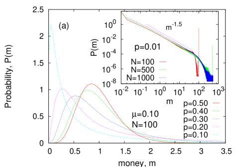
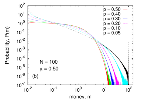
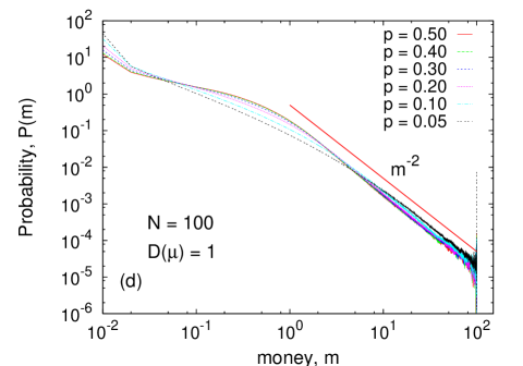
Figure 2: The steady state distribution $P(m)$ of money $m$ for directed networks characterized by different values of $p$. (a) For $\mu=0.1$, the inset shows $P(m)$ for $p=0.01$ for $N=100,500,1000$, and the power law $m^{-1.5}$ is also indicated. (b) For $\mu=0.5$ and (c) $\mu=0.9$. (d) shows the plots for uniform, random distributed $\mu$, $D(\mu)=1$, and also a guide to the power law $m^{-2}$. The data are obtained by numerical simulation, for a system of $N=100$ nodes, averaged over $10^{3}$ realizations in the steady state and over $10^{4}$ initial configurations. The average money $M/N$ is $1$.

The rules of exchange are as follows: If $a_{ij}=-1$,

$$m_{i}(t+1) = m_{i}(t)+\mu_{j}m_{j}(t)$$

$$m_{j}(t+1) = m_{j}(t)-\mu_{j}m_{j}(t)$$

else, $a_{ij}=+1$,

$$m_{i}(t+1) = m_{i}(t)-\mu_{i}m_{i}(t)$$

$$m_{j}(t+1) = m_{j}(t)+\mu_{i}m_{i}(t).$$

where $0<\mu_{i}<1$ is a ‘transfer fraction’ associated with the $i$th agent, and $m_{i}(t)$ is the money of agent $i$ (or, money at node $i$) at time $t$. The total money in the system is conserved, no money is created or destroyed, as is evident from eqn. (III.1) and eqn. (III.1). If there is a link from $j$ to $i$, the node $i$ gains $\mu_{j}$ fraction of $j$th agent’s money, which, of course agent $j$ loses. Otherwise, if there is a link from $i$ to $j$, the node $j$ gains $\mu_{i}$ fraction of $i$th agent’s money, which, of course agent $i$ loses. In the Monte Carlo simulations, one assigns random amount of money to agents to start with, such that the average money $M/N=1$. A pair of agents (nodes) are chosen at random, and depending on the directionality of the link between them (the sign of $a_{ij}$), the relevant rule, eqn. (III.1) or eqn. (III.1) is chosen. This is repeated until a steady state is reached and the distribution of money does not change in time. The distribution of money $P(m)$ is obtained by averaging over several ensembles (different random initial distribution of money).

This model is different from the CC and CCM models, but one can relate the transfer fraction $\mu$ analogous to $\lambda$ in the CC and CCM models.

III.2 Model with uniform $\mu$

First we discuss the case of homogeneous agents, i.e, when all agents $i$ have $\mu_{i}=\mu$. The $\mu=0$ limit is trivial, as the system does not perform any dynamics. Fig. 2(a) shows the steady state distribution $P(m)$ of money $m$ for $\mu=0.1$ for different values of network disorder $p$. In general, the distribution of money has a most probable value, which shifts monotonically from about $0.85$ for $p=0.5$ to $0$ as $p\to 0$. $P(m)$ has an exponential tail, but a power law region develops as $p\to 0$ in between the most probable peak and the exponential cut-off, which fits approximately to $m^{-1.5}$. For the limit $p\to 0$, condensation of wealth at the node(s) with strong disorder ($\rho\to 1$) is apparent from the single, isolated data point at the $m_{max}=M$ end (see inset of Fig. 2(a), for $p=0.01$). There is a strong finite size effect involved in this behavior. To emphasize this, we plot $P(m)$ for $p=0.01$ for $N=100,500$ and $1000$ (inset of Fig. 2(a)). While $N=100$ and $N=500$ does show the isolated data point, it is absent for $N=1000$. This indicates that this behavior is absent for infinite systems for $p\to 0$. For larger values of $p$, the distribution resembles Gamma distributions, as in the CC model. For $\mu=0.5$, the most-probable value of $P(m)$ is always at $0$ (see Fig. 2(b)). For weak disorder ($p=0.5$), $P(m)$ is exponential, but it goes to a wider distribution as one goes to higher disorder ($p\to 0$). The condensation of wealth at node(s) with high value of $\rho$ ($\rho\to 1)$ is again apparent from the single, isolated data point at the $m_{max}=M$ end (see Fig. 2(b), for $p=0.05$). For $\mu=0.9$, $P(m)$ is always decaying, with a wide distribution upto $m_{max}=M$ (see Fig. 2(c)). As like previous plots, the condensation of wealth at node(s) with high value of $\rho$ is visible: see plot for $p=0.05$ in Fig. 2(c). A common feature for the curves for all values of $p$ is that, $P(m)$ exhibits log-periodic oscillations, while resembling roughly a power-law decay. Another important feature is that $P(m)\to N$ for $m\to 0$, which indicates that money is distributed in a very small fraction of nodes, while most nodes have almost no money at a given instance.

For a particular value of the network disorder $p$, the wealth distribution $P(m)$ becomes more and more ‘fat tailed’ as $\mu$ is increased. This is in contrast to what is observed in CC model Chakraborti:2000 where $P(m)$ organizes to a narrower distribution as $\lambda$ increases.

III.3 Model with distributed $\mu$

We now consider the case when agents $i$ have have different values of $\mu_{i}$, which do not change in time. This is a case of heterogeneous agents where the heterogeneity can be viewed as a ‘quenched disorder’. We consider a random uniform distribution of $\mu$, i.e, $D(\mu)=1$ in $0<\mu<1$. This is the case analogous to the CCM model Chatterjee:2004 . Fig. 2(d) shows the plots of the money distribution $P(m)$ for different values of network disorder $p$. All curves have a power law tail, resembling a $m^{-2}$ variation. However, the effect of the topology of the underlying network are visible: For strong disorder in topology $p=0.05$, condensation of wealth at node(s) with high value of $\rho$ ($\rho\to 1)$ is also apparent from the single, isolated data point at the $m_{max}=M$ end. Further investigations also indicate that the power law exponent is similarly related to the distribution of ‘transfer fraction’ $\mu$, as one observes in the CCM model Chatterjee:2004 ; Mohanty:2006 , i.e, $P(m)\sim m^{-2}$ for most distributions, while one can obtain $P(m)\sim m^{-(2+\delta)}$ if $D(\mu)\propto(1-\mu)^{\delta}$.

IV Discussions

The empirical data for income and wealth distribution in many countries are now available, and they reflect a particular robust pattern: The bulk (about 90%) of the distribution resemble the century-old Gibbs distribution of energy for an ideal gas, while there are evidences of considerable deviation in the low income as well as high income ranges. The high income range data (for 5-10% of the population in any country) fits to a power law tail, known after Pareto, and the value of the (power law) exponent ranges between 1-3 and depends on the individual make-up of the economy of the society or country.

The analogy with a gas like many-body system has led to the formulation of the models of markets. The random scattering-like dynamics of money (and wealth) in a closed trading market, in analogy with energy conserved exchange models, reveals interesting features. Self-organization is a key emerging feature of these kinetic exchange models when saving factors are introduced. These models Chakraborti:2000 ; Chatterjee:2004 produce asset distributions resembling that observed in reality, and are quite well studied now Chatterjee:rev . Empirical observations in homogeneous groups of individuals as in waged income of factory labourers in UK and USA Willis:2004 and data from population survey in USA among students of different school and colleges produce similar distributions Angle:2006 . There have also been other models Sinha:2003 which uses the kinetic exchange approach.

Heterogeneity is an inherent feature of real networked economy, mostly observed with with behavior of agents contributing to irreversible flow of money. A simple way of looking into it is to consider heterogeneity in the interaction topology for the agents. In all earlier studies, the effect of the topology of the space on which the kinetic exchanges took place, was overlooked. Most of the models were either on regular, undirected lattices, or on undirected graphs. Our study concentrates on the effect of a directed network as the exchange space for such kinetic exchanges. We consider a simple, fully connected, directed network. A notion of disorder $\rho$ in the directedness of the graph was introduced, in analogy to real world networks, which depend on the number of incoming and outgoing links at a particular node. The distribution $R(\rho)$ characterizes a particular network. In analogy to saving propensity $\lambda$ in CC and CCM models Chakraborti:2000 ; Chatterjee:2004 , we define a ‘transfer fraction’ $\mu$. We consider two distinct models: (i) with uniform $\mu$ (Sec. III.2), and (ii) with distributed $\mu$ (Sec. III.3). We employ numerical simulations to study the above models. For uniform $\mu$, when the transfer fraction $\mu$ is small, low degree of disorder in the network produced money distribution $P(m)$ with most-probable money at finite values of $m$ similar to Gamma distribution observed in CC model Chakraborti:2000 , while high disorder produced a wider distribution of $P(m)$ (Fig. 2(a)). At intermediate ranges of $\mu$, $P(m)$ has its most-probable value always at $m\to 0$ (Fig. 2(b)), while for high values of $\mu$, $P(m)$ has a wide distribution with log-periodic oscillations (Fig. 2(c)). For the model with $\mu$ distributed randomly and uniformly ($D(\mu)=1$), money distribution exhibits power law $P(m)\sim m^{-2}$ for large money $m$ (Fig. 2(d)). The common feature of all these cases was a very wide distribution $P(m)$ of money, when the network disorder is very strong (see plots for $p=0.05$ in Fig. 2), accompanied by a signature of accumulation of money at the nodes/with the agents having strongest disorder, which is observed in the data point at $m_{max}=M$. However, this effect is more pronounced in smaller system sizes, while it may disappear in the thermodynamic limit (see inset of Fig. 2(a)).

A simple model of similar exchanges have been studied before Dragulescu:2000 . The case corresponds to the choice $p=0.5$ for our model. Moreover, the transferred money was independent of $m$ and not proportional to $\mu$. Money distribution was found to be exponential despite explicit violation of time-reversal symmetry. In an earlier paper Ispolatov:1998 , results for multiplicative random exchanges correspond to certain cases of the present paper. It was found that $P(m)$ vanishes at $m=0$ for $\mu<0.5$ and diverges for $\mu>0.5$, and is exponential for $\mu=0.5$. These results correspond to that of our model for $p=0.5$ (Sec. III.2).

We have mostly used the terms ‘money’ and ‘wealth’ interchangeably, treating the models in terms of only one quantity, namely ‘money’ that is exchanged. Of course, wealth does not comprise of (paper) money only, and there have been studies distinguishing these two Chatterjee:rev ; Silver:2002 ; Ausloos:2007 .

Study of such simple models here give some insight into the possible emergence of self organizations in such markets, evolution of the steady state distribution, emergence of Gamma-like distribution for the bulk and of the power law tail, as in the empirically observed distributions. The study of models on directed graphs gives us new insights: (i) one can obtain wide asset distribution even in homogeneous populations (as in uniform $\mu$), (ii) the power law exponent for the distributed $\mu$ case behaves in the same manner as in CCM model, and (iii) strong disorder in topology of the underlying directed network produces accumulation (at $\rho\to 1$) or the opposite effect (at $\rho\to-1$) of wealth, thus giving rise to a higher degree of wealth inequality in the system.

These model studies also indicate the appearance of self-organization, and the self-organized criticality Bak:1997 in particular, in the simple models. These have prospective applications in other spheres of social science, as in application in policy making and taxation, and also physical sciences, in designing desired energy spectrum for different types of chemical reactions Scafetta:2007 .

- (1) V. Pareto, Cours d’economie Politique, F. Rouge, Lausanne (1897).
- (2) B. B. Mandelbrot, Int. Econ. Rev. 1 (1960) 79.
- (3) A. Chatterjee, S. Yarlagadda, B. K. Chakrabarti (Eds.), Econophysics of Wealth Distributions, Springer Verlag, Milan (2005).
- (4) B. K. Chakrabarti, A. Chakraborti, A. Chatterjee (Eds.), Econophysics and Sociophysics, Wiley-VCH, Berlin (2006).
- (5) P. Richmond, S. Hutzler, R. Coelho, P. Repetowicz, in Ref. ESTP .
- (6) A. C. Silva, V. M. Yakovenko, Europhys. Letts., 69 (2005) 304; Ref. EWD05 .
- (7) G. Willis, J. Mimkes, cond-mat/0406694.
- (8) A. A. Drăgulescu, V. M. Yakovenko, Eur. Phys. J. B, 20 (2001) 585.
- (9) A. A. Drăgulescu, V. M. Yakovenko, Physica A 299 (2001) 213.
- (10) M. Levy, S. Solomon, Physica A 242 (1997) 90.
- (11) S. Sinha, Physica A 359 (2006) 555.
- (12) H. Aoyama, W. Souma, Y. Fujiwara, Physica A 324 (2003) 352.
- (13) T. Di Matteo, T. Aste, S. T. Hyde, in The Physics of Complex Systems (New Advances and Perspectives), F. Mallamace, H. E. Stanley (Eds.), Amsterdam (2004), p. 435.
- (14) F. Clementi, M. Gallegati, Physica A 350 (2005) 427; EWD05 .
- (15) N. Ding, Y. Wang, Chinese Phys. Letts., 24 (2007) 2434.
- (16) B. K. Chakrabarti, S. Marjit, Ind. J. Phys. B 69 (1995) 681;
- (17) S. Ispolatov, P. L. Krapivsky, S. Redner, Eur. Phys. J. B 2 (1998) 267.
- (18) A. A. Drăgulescu, V. M. Yakovenko, Eur. Phys. J. B 17 (2000) 723.
- (19) A. Chakraborti, B. K. Chakrabarti, Eur. Phys. J. B 17 (2000) 167.
- (20) B. K. Chakrabarti, A. Chatterjee, in Application of Econophysics, H. Takayasu (Ed.), Springer, Tokyo (2004) pp. 280
- (21) P. A. Samuelson, Economics, Mc-Graw Hill Int., Auckland (1980).
- (22) M. Patriarca, A. Chakraborti, K. Kaski, Phys. Rev. E 70 (2004) 016104.
- (23) P. Repetowicz, S. Hutzler, P. Richmond, Physica A 356 (2005) 641.
- (24) J. Angle, Social Forces 65 (1986) 293.
- (25) J. Angle, Physica A 367 (2006) 388.
- (26) A. Chatterjee, B. K. Chakrabarti, S. S. Manna, Physica A 335 (2004) 155; Phys. Scripta T 106 (2003) 36.
- (27) P. K. Mohanty, Phys. Rev. E 74 (2006) 011117.
- (28) A. Chatterjee, B. K. Chakrabarti, Eur. Phys. J. B 54 (2006) 399; Eur. Phys. J. B 60 (2007) 135; A. Chatterjee, S. Sinha, B. K. Chakrabarti, Current Science 92 (2007) 1383.
- (29) K. E. Dynan, J. Skinner, S. P. Zeldes, J. Pol. Econ. 112 (2004) 397.
- (30) A. Chatterjee, B. K. Chakrabarti, R. B. Stinchcombe, Phys. Rev. E 72 (2005) 026126.
- (31) A. Chatterjee, B. K. Chakrabarti, Physica A 382 (2007) 36-41.
- (32) S. Wassermann, K. Faust, Social network analysis, Cambridge Univ. Press, Cambridge (1994).
- (33) R. Albert, A.-L. Barabási, Rev. Mod. Phys. 74 (2002) 47.
- (34) S. N. Dorogovtsev, J. F. F. Mendes, Evolution of Networks: From Biological Nets to the Internet and WWW, Oxford Univ. Press, Oxford (2003).
- (35) M-B. Hu, W-X. Wang, R. Jiang, Q-S. Wu, B-H. Wang, Y-H. Wu, Eur. Phys. J. B, 53 (2006) 273.
- (36) M-B. Hu, R. Jiang, Q-S. Wu, Y-H. Wu, Physica A, 381 (2007) 476.
- (37) D. Garlaschelli, M. I. Loffredo, J. Phys. A: Math. Theor. 41 (2008) 224018.
- (38) S. Sinha, Phys. Scripta T 106 (2003) 59; M. A. Saif, P. M. Gade, Physica A, 384 (2007) 448; H. Yuqing, Physica A 377 (2007) 230; N. Ding, N. Xi, Y. Wang, Eur. Phys. J. B 36 (2003) 149; B. Düring, G. Toscani, Physica A 384 (2007) 493; F. Slanina, Phys. Rev. E 69 (2004) 046102.
- (39) M. Ausloos, A. Peķalski, Physica A 373 (2007) 560.
- (40) J. Silver, E. Slud, K. Takamoto, J. Econ. Theory 106 (2002) 417.
- (41) P. Bak, How Nature works, Oxford University Press, Oxford (1997).
- (42) N. Scafetta, B. J. West, J. Phys: Cond. Matter 19 (2007) 065138.