Variability type classification of multi-epoch surveys
Abstract
The classification of time series from photometric large scale surveys into variability types and the description of their properties is difficult for various reasons including but not limited to the irregular sampling, the usually few available photometric bands, and the diversity of variable objects. Furthermore, it can be seen that different physical processes may sometimes produce similar behavior which may end up to be represented as same models. In this article we will also be presenting our approach for processing the data resulting from the Gaia space mission. The approach may be classified into following three broader categories: supervised classification, unsupervised classifications, and ”so-called” extractor methods i.e. algorithms that are specialized for particular type of sources. The whole process of classification- from classification attribute extraction to actual classification- is done in an automated manner.
Keywords:
Quasars, Variable stars:
95.10.Gi, 95.75.De, 95.75.Fg, 95.75.Pq, 95.75.Wx, 95.85.Kr, 97.10.Jb, 97.10.Kc, 97.10.Sj, 97.10.Vm, 97.10.Yp, 97.10.Zr, 97.30.-b, 97.80.-d, 98.54.-h1 Variability physical types and variability behaviours
The classification of variable objects is necessarily based on the observable attributes. The lightcurve behaviour is the main parameter but some other source characteristics -such as mean absolute luminosity and mean colour- are equally useful. The ultimate goal is however to try to separate sources into physical categories as a first step towards learning more about the nature of the source and the causes for variability. Reaching this goal is complicated by the fact that some very different physical processes can generate similar variability behaviours. For example, two pulsating stars may end up having different models to describe them, while two different physical process may be described by the same models e.g. EW eclipsing binaries and some mono-periodic pulsating stars.
The general-purpose classification may then be confused being unable to disentangle two or more physical categories. Obviously a refined analysis may unravel the physical process, such as the analysis of luminosity, temperature, behaviours at different wavelengths etc. Therefore we have introduced a specific object studies module, whose goal is to validate and refine the results of the general-purpose classification process.
Eyer and Mowlavi Eyer and Mowlavi (2007) proposed a tentative organisation of variability physical types into a tree structure. The variability behaviours on the other hand, can be at the high-level, be divided into different categories i.e. periodic, semi-regular, irregular, and transient. The time scale and amplitude of the variation can be very different: from event as short as a few seconds to secular evolution and from milli-magnitudes to several magnitudes.
2 Survey properties
Different surveys have different properties such as photometric bands, random and systematic photometric errors, time sampling, possible crowding issues, etc. These specific properties can be exploited as well as possible through the data analysis in order to learn more about the physical processes at the origin of the variability. Here we consider the time sampling properties only.
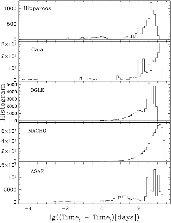
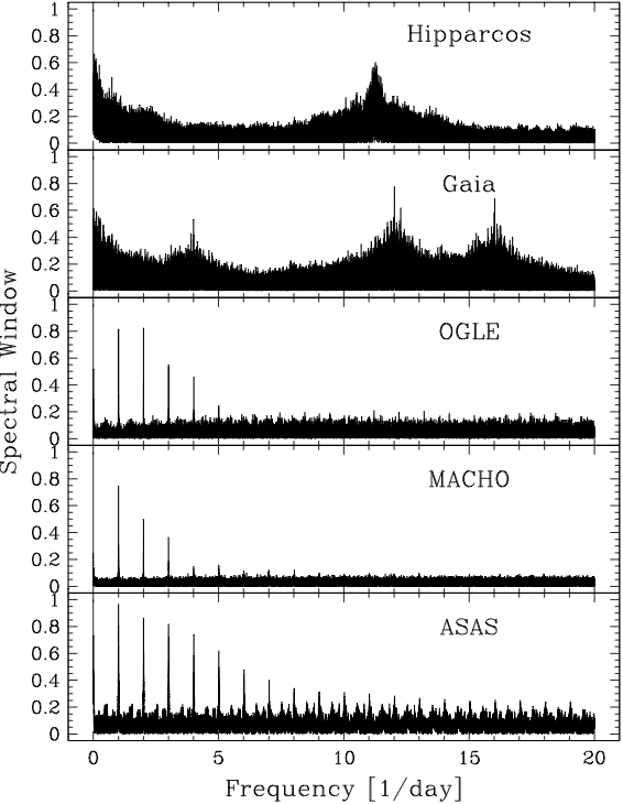
There are two important ways to assess the quality of the time sampling: the time-lag histogram and the spectral window.
A time-lag histogram is built from all possible time differences ( such that ) between pair of measurements of a given lightcurve. The time-lag histogram shows which delta times, and hence which variability timescales, are probed by a set of measurements. This is most useful to predict the ability of a survey to characterise transient or irregular variability behaviour of a given characteristic variation time.
The spectral window is the Fourier transform of the set of sampling times. There are two extreme cases. If the measurements are taken at regular time interval, the Fourier transform will exhibit series of strong peaks spaced by the frequency corresponding to this time interval. If, on the other hand, the time sampling is random, there will be no peak in the spectral window but a rather smooth continum. The Fourier transform of the signal is the convolution of the source signal with the spectral window. A mono-periodic source is a single spike in the Fourier domain, and in this case the Fourier transform of the signal has the shape of the spectral windows, but it is just shifted in frequency by the source frequency value. This allows to confirm our intuition: a random sampling will be much better for detecting periods. Note that period much smaller that the smallest time lag can in principle be recovered if the signal accuracy is high and the spectral window good Eyer and Bartholdi (1999).
Both the time-lag histogram and the spectral window from several surveys (Hipparcos, Gaia, OGLE, MACHO and ASAS) are represented in Fig. 1. For each case a random time series has been used to produce the diagrams. These surveys appear to have very different properties. Hipparcos and Gaia have similar spectral windows. They are quite good for period search as they show no strong secondary peaks. The global ”noise” level is however higher because of the smaller number of measurements. In the other single site ground-based surveys, we see the peaks produced by the 1/day observation frequency, strongest in the case of ASAS. These figure allow us to better understand why Hipparcos was so successful in discovering complex objects like Dor and SPB stars with periods between 1-3 days.
3 Some examples of classification methods applied to surveys
Many studies based on microlensing searches focused on a given variable type and ”extract” objects of this particular type using a priori knowledge about their variability properties. Variability types are extracted and studied independently and sequentially. Such a scheme is followed in most OGLE or MACHO studies. Others approaches based on global classification algorithms have started to flourish during this past decade. The goal of this section is not to go through all classification methods that appeared in the literature, but rather to show the diversity of approaches, using different sets of attributes or classification methods. To our knowledge, Waelkens et al. (1998) presented the first analysis which tackled a fully automated classification on a whole sky survey. It was however limited to a rather small sample of B stars. Using the combined information of characterisation of Hipparcos time series (such as main period, amplitude in Hp band) and Geneva multicolour photometry, and applying a multivariate discriminant analysis, the Hipparcos B stars were classified into Cep, SPB and Chemically Peculiar stars, and also as eclipsing binaries. As far as classification attributes are concerned, Evans and Belokurov (2004) proposed to work in the Fourier space by defining an envelope of the power spectrum of the signal. Wyrzykowski et al. Wyrzykowski et al. (2003), Wyrzykowski et al. (2004) used a neural network on the images of the folded time series. In the case of ASAS, Pojmanski and Maciejewski Pojmanski and Maciejewski (2004) have set up an automated pipeline. First they separate the stricly periodic objects with respect to the less regular ones and then they use the attributes from the ASAS light curve and 2MASS colours to perform the classification using the variability types properties in ad-hoc selected projected 2D planes. Eyer & Blake Eyer and Blake (2002), Eyer and Blake (2005) used an unsupervised classification method (Autoclass) applied on a Fourier modelling of the light curves of ASAS data.
4 Plan for the Gaia mission
CU7 is the Coordination Unit, part of the Gaia ground-based data processing and analysis consortium (cf. Mignard et al. (2008)), in charge of all aspects of the analysis of the measurement of variability. One of the most important tasks in this context is the classification of the sources according to their lightcurve behaviour. The classification is structured into a three step process (1) a number of attributes are first computed to characterise the lightcurves, (2) these attributes are then fed into the classification algorithms, and (3) finally specific processing is applied to the sources of each of the different groups obtained through step 2 to validate and possibly refine the classification result. The different types of classification algorithms considered are categorised into (1) supervised, (2) unsupervised, and (3) extractor methods.
Supervised classification. In the frame of supervised methods, the most important factor is that of finding best attributes in order to build the training set for classification algorithms. The strategy is to iteratively refine the training set by using different attribute/method combinations, then comparing the result. The most meaningful attribute set, both in terms of separation power and independence, can thus gradually be derived.
Although the training set data may be derived from the theoretical model, the current approach is to rely on the data from existing surveys and by utilizing the work of Debosscher et al. (2007) done in the context of the COROT mission. Following two steps are identified in order to build a representative training set for the Gaia variability classification task: firstly, a list of sources representing different variability class is to be established; secondly, lighcurves, similar to the ones obtained by the Gaia mission, must be collected for selected source classes from the existing data. For the second step, we will eventually be able to use Gaia measurements during the mission as well. The final training set is likely to emerge from the iterative process as described above. In this regards, a multi-stage approach design by Sarro et al. (2008), is being explored. The multi stage classifier breaks the classification problem into various stages, each classifying a specific set of source class possibly using different attribute sets. The main advantage of this approach is that the attribute sets and the classification schemes used at various stages could possibly be completely different for each stage
Unsupervised classification. The challenge of the unsupervised classification with the Gaia data may well come from the potentially large number of variable sources most probably of the order of . One of the first tasks is to evaluate as to how many sources can be fed into existing algorithms with currently available hardware and then to try to extrapolate the results to the hardware that will eventually be available during the mission. We may need to investigate algorithms that offer support for processing data in sub-samples in one way or another before aggregating the results. We also consider new time series indexing techniques to obtain intrinsic clustering directly in our data storage system with possibility of exploring novel data mining approaches in very large databases. This may reduce the need for linear increase in demand for RAM, needed in a brute force approach.
Extractors. Extractors are tools that take advantage of the knowledge gained about the lightcurve behaviours for certain types of variable stars. Scanning the complete set of variable objects, they try to identify specific lightcurve behaviours, and thus they can “extract” sources of a given class. The current list of extractors that CU7 plan to develop includes: (1) Microlensing events, (2) Flare Stars.
Specific Object Studies (SOS). Once the sources have been classified by general algorithm into classes, we plan to carry out a specific processing for each of the classes. Two important goals of the SOS processing is to validate and refine the results of the classification.
4.1 Classification of Hipparcos sources
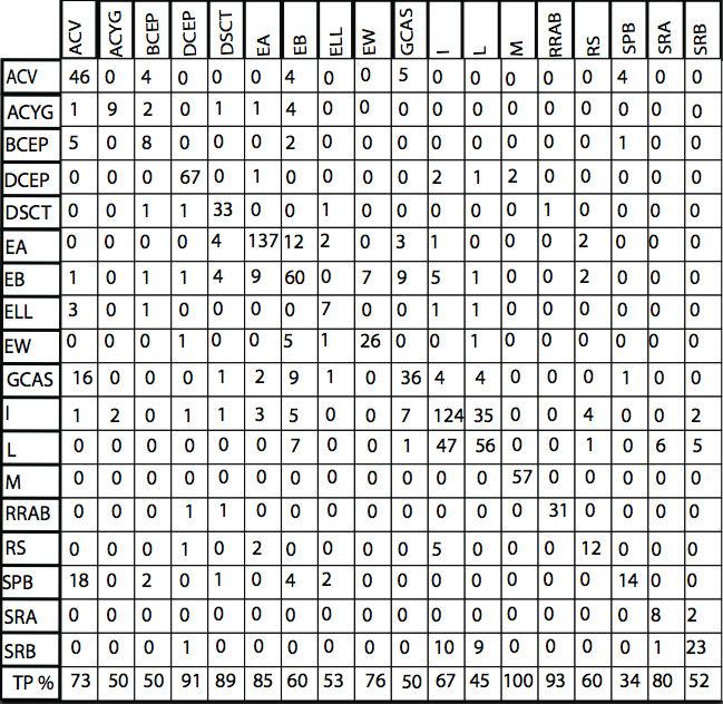
Of all the available surveys, Hipparcos shares most of the aspects of the Gaia mission i.e. the global sky survey, astrometric information, its peculiar sampling etc. Furthermore, till date the whole Hipparcos data has not been classified in a systematic way; the previous studies ESA (1997), Waelkens et al. (1998) and Aerts et al. (1998) either employed visual inspection methods for classification or investigated objects from specific (sub)classes. Willemsen and Eyer (2007) presented the results of first ever systematic global classification of the Hipparcos data, using support vector machine, and formed basis for the current study. We employed a two approaches in order to undertake the classification task. In one approach, we utilized the attribute sets as established by Willemsen and Eyer (2007) and in other approach the characterization module, part of CU7 software framework, was used to extract key attributes from the Hipparcos light curves. Some of the important attributes include standard deviation (weighted), skewness (weighted), kurtosis (weighted), normalized p2p scatter (weighted), slope, log frequency, amplitude, phase, log amplitude, range and log range, B-V and V-I. The classification models were obtained using support vector machine algorithm being part of Weka machine learning library, and were applied using CU7 classification module. It may be noted that using the current implementation of CU7 software framework, the complete process of extracting classification attributes, and performing classification can be done in a completely automated manner. We used different strategies to validate the classifier result i.e. using n-fold cross validation as well as doing a percentage split of the available data in the training and test sets. Using a training set of 2100 objects and a test set of 1100 objects, a classification accuracy of nearly 68 percent was achieved, with more than 9 classes having an accuracy well above 70 percent (i.e. above 90 percent in some cases). The following table summarizes the confusion matrix for the classifier obtained using the attributes from Willemsen and Eyer (2007), the confusion matrix obtained using CU7 characterization module was also similar to the one displayed in Fig 2.
References
- Eyer and Mowlavi (2007) L. Eyer, and N. Mowlavi, ArXiv e-prints (2007), 0712.3797.
- Eyer and Bartholdi (1999) L. Eyer, and P. Bartholdi, Astronomy and Astrophysics Supplement 135, 1–3 (1999), arXiv:astro-ph/9808176.
- Waelkens et al. (1998) C. Waelkens, C. Aerts, E. Kestens, M. Grenon, and L. Eyer, Astronomy and Astrophysics 330, 215–221 (1998).
- Evans and Belokurov (2004) N. W. Evans, and V. Belokurov, ArXiv Astrophysics e-prints (2004), arXiv:astro-ph/0411439.
- Wyrzykowski et al. (2003) L. Wyrzykowski, A. Udalski, M. Kubiak, M. Szymanski, K. Zebrun, I. Soszynski, P. R. Wozniak, G. Pietrzynski, and O. Szewczyk, Acta Astronomica 53, 1–25 (2003), arXiv:astro-ph/0304458.
- Wyrzykowski et al. (2004) L. Wyrzykowski, A. Udalski, M. Kubiak, M. K. Szymanski, K. Zebrun, I. Soszynski, P. R. Wozniak, G. Pietrzynski, and O. Szewczyk, Acta Astronomica 54, 1– (2004), arXiv:astro-ph/0404523.
- Pojmanski and Maciejewski (2004) G. Pojmanski, and G. Maciejewski, Acta Astronomica 54, 153–179 (2004), arXiv:astro-ph/0406256.
- Eyer and Blake (2002) L. Eyer, and C. Blake, “Automated Classification of Variable Stars for ASAS Data,” in IAU Colloq. 185: Radial and Nonradial Pulsationsn as Probes of Stellar Physics, edited by C. Aerts, T. R. Bedding, and J. Christensen- Dalsgaard, 2002, vol. 259 of Astronomical Society of the Pacific Conference Series, pp. 160–+.
- Eyer and Blake (2005) L. Eyer, and C. Blake, Monthly Notices of the Royal Astronomical Society 358, 30–38 (2005), arXiv:astro-ph/0406333.
- Mignard et al. (2008) F. Mignard, C. Bailer-Jones, U. Bastian, R. Drimmel, L. Eyer, D. Katz, F. van Leeuwen, X. Luri, W. O’Mullane, X. Passot, D. Pourbaix, and T. Prusti, “Gaia: organisation and challenges for the data processing,” in IAU Symposium, 2008, vol. 248 of IAU Symposium, pp. 224–230.
- Debosscher et al. (2007) J. Debosscher, L. M. Sarro, C. Aerts, J. Cuypers, B. Vandenbussche, R. Garrido, and E. Solano, Astronomy and Astrophysics 475, 1159–1183 (2007), 0711.0703.
- Sarro et al. (2008) L. M. Sarro, J. Debosscher, M. Lopez, and C. Aerts, ArXiv e-prints (2008), 0806.3386.
- ESA (1997) ESA, ESA SP-1200 (1997).
- Aerts et al. (1998) C. Aerts, L. Eyer, and E. Kestens, Astronomy and Astrophysics 337, 790–796 (1998).
- Willemsen and Eyer (2007) P. G. Willemsen, and L. Eyer, ArXiv e-prints (2007), 0712.2898.