A process very similar to multifractional Brownian motion

Abstract : Multifractional Brownian motion (mBm), denoted here by $X$, is one of the paradigmatic examples of a continuous Gaussian process whose pointwise Hölder exponent depends on the location. Recall that $X$ can be obtained (see e.g. BJR (97); AT (05)) by replacing the constant Hurst parameter $H$ in the standard wavelet series representation of fractional Brownian motion (fBm) by a smooth function $H(\cdot)$ depending on the time variable $t$. Another natural idea (see BBCI (00)) which allows to construct a continuous Gaussian process, denoted by $Z$, whose pointwise Hölder exponent does not remain constant all along its trajectory, consists in substituting $H(k/2^{j})$ to $H$ in each term of index $(j,k)$ of the standard wavelet series representation of fBm. The main goal of our article is to show that $X$ and $Z$ only differ by a process $R$ which is smoother than them; this means that they are very similar from a fractal geometry point of view.

Keywords: Fractional Brownian motion, wavelet series expansions, multifractional Brownian motion, Hőlder regularity.

1 Introduction and statement of the main results

Throughout this article we denote by $H(\cdot)$ an arbitrary function defined on the real line and with values in an arbitrary fixed compact interval $[a,b]\subset(0,1)$. We will always assume that on each compact ${\cal K}\subset\hbox{\it I\hskip-2.0ptR}$, $H(\cdot)$ satisfies a uniform Hőlder condition of order $\beta>b$ i.e. there is a constant $c_{1}>0$ (which a priori depends on ${\cal K}$) such that for every $t_{1},t_{2}\in{\cal K}$ one has,

$$|H(t_{1})-H(t_{2})|\leq c_{1}|t_{1}-t_{2}|^{\beta};$$ (1)

typically $H(\cdot)$ is a Lipschitz function over IR. We will also assume that $a=\inf\{H(t)\,:\,t\in\hbox{\it I\hskip-2.0ptR}\}$ and $b=\sup\{H(t)\,:\,t\in\hbox{\it I\hskip-2.0ptR}\}$. Recall that multifractional Brownian motion (mBm) of functional parameter $H(\cdot)$, which we denote by $X=\{X(t):\,\,t\in\hbox{\it I\hskip-2.0ptR}\}$, is the continuous and nowhere differentiable Gaussian process obtained by replacing the Hurst parameter in the harmonizable representation of fractional Brownian motion (fBm) by the function $H(\cdot)$. That is, the process $X$ can be represented for each $t\in\hbox{\it I\hskip-2.0ptR}$ as the following stochastic integral

$$X(t)=\int_{\hbox{\it I\hskip-2.0ptR}}\frac{e^{it\xi}-1}{|\xi|^{H(t)+1/2}}\,d\widehat{W}(\xi),$$ (2)

where $d\widehat{W}$ is “the Fourier transform” of the real-valued white-noise $dW$ in the sense that for any function $f\in L^{2}(\hbox{\it I\hskip-2.0ptR})$ one has a.s.

$$\int_{\hbox{\it I\hskip-2.0ptR}}f(x)\,dW(x)=\int_{\hbox{\it I\hskip-2.0ptR}}\widehat{f}(\xi)\,d\widehat{W}(\xi).$$ (3)

Observe that (3) implies that (see C (99); ST (06)) the following equality holds a.s. for every $t$, to within a deterministic smooth bounded and non-vanishing deterministic function,

$$\int_{\hbox{\it I\hskip-2.0ptR}}\frac{e^{it\xi}-1}{|\xi|^{H(t)+1/2}}\,d\widehat{W}(\xi)=\int_{\hbox{\it I\hskip-2.0ptR}}\Big{\{}|t-s|^{H(t)-1/2}-|s|^{H(t)-1/2}\Big{\}}\,dW(s).$$

Therefore $X$ is a real-valued process. MBm was introduced independently in PLV (95) and BJR (97) and since then there is an increasing interest in the study of multifractional processes, we refer for instance to FaL ; S (08) for two excellent quite recent articles on this topic. The main three features of mBm are the following:

• $X$ reduces to a fBm when the function $H(\cdot)$ is constant.

• Unlike to fBm, $\alpha_{X}=\{\alpha_{X}(t):\,\,t\in\hbox{\it I\hskip-2.0ptR}\}$ the pointwise Hölder exponent of $X$ may depend on the location and can be prescribed via the functional parameter $H(\cdot)$; in fact one has (see PLV (95); BJR (97); AT (05); AJT (07)) a.s. for each $t$,

  $$\alpha_{X}(t)=H(t).$$ (4)

  Recall that $\alpha_{X}$ the pointwise Hölder exponent of an arbitrary continuous and nowhere differentiable process $X$, is defined, for each $t\in\hbox{\it I\hskip-2.0ptR}$, as

  $$\alpha_{X}(t)=\sup\left\{\alpha\in\hbox{\it I\hskip-2.0ptR}_{+}:\,\,\limsup_{h\rightarrow 0}\frac{|X(t+h)-X(t)|}{|h|^{\alpha}}=0\right\}.$$ (5)

• At any point $t\in\hbox{\it I\hskip-2.0ptR}$, there is an fBm of Hurst parameter $H(t)$, which is tangent to mBm BJR (97); F (02, 03) i.e. for each sequence $(\rho_{n})$ of positive real numbers converging to $0$, one has,

  $$\lim_{n\rightarrow\infty}\mbox{law}\left\{\frac{X(t+\rho_{n}u)-X(t)}{\rho_{n}^{H(t)}}:\,\,u\in\hbox{\it I\hskip-2.0ptR}\right\}=\mbox{law}\{B_{H(t)}(u):\,\,u\in\hbox{\it I\hskip-2.0ptR}\},$$ (6)

  where the convergence holds in distribution for the topology of uniform convergence on compact sets.

The main goal of our article is to give a natural wavelet construction of a continuous and nowhere differentiable Gaussian process $\displaystyle Z=\{Z(t)\}_{t\in\hbox{\it I\hskip-2.0ptR}}$ which has the same features $(a)$, $(b)$ and $(c)$ as mBm $X$ and which differs from it by a smoother stochastic process $R=\{R(t):\,\,t\in\hbox{\it I\hskip-2.0ptR}\}$ (see Theorem 1.1).

In order to be able to construct $Z$, first we need to introduce some notation. In what follows we denote by $\{2^{j/2}\psi(2^{j}x-k):\,\,(j,k)\in\hbox{\it Z\hskip-4.0ptZ}^{\,2}\}$ a Lemarié-Meyer wavelet basis of $L^{2}(\hbox{\it I\hskip-2.0ptR})$ LM (86) and we define $\Psi$ to be the function , for each $(x,\theta)\in\hbox{\it I\hskip-2.0ptR}\times\hbox{\it I\hskip-2.0ptR}$,

$$\Psi(x,\theta)=\int_{\hbox{\it I\hskip-2.0ptR}}e^{ix\xi}\frac{\widehat{\psi}(\xi)}{|\xi|^{\theta+1/2}}\,d\xi.$$ (7)

By using the fact that $\widehat{\psi}$ is a compactly supported $C^{\infty}$ function vanishing on a neighborhood of the origin, it follows that $\Psi$ is a well-defined $C^{\infty}$ function satisfying for any $(l,m,n)\in\hbox{\it I\hskip-2.0ptN}^{\,3}$ with $l\geq 2$, the following localization property (see AT (05) for a proof),

$$c_{2}=\sup_{\theta\in[a,b],\,x\in\hbox{\it I\hskip-2.0ptR}}(2+|x|)^{\ell}|(\partial_{x}^{m}\partial_{\theta}^{n}\Psi)(x,\theta)|<\infty,$$ (8)

where $\partial_{x}^{m}\partial_{\theta}^{n}\Psi$ denotes the function obtained by differentiating the function $\Psi$, $n$ times with respect to the variable $\theta$ and $m$ times with respect to the variable $x$. For convenience, let us introduce the Gaussian field $B=\{B(t,\theta):\,\,(t,\theta)\in\hbox{\it I\hskip-2.0ptR}\times(0,1)\}$ defined for each $(t,\theta)\in\hbox{\it I\hskip-2.0ptR}\times(0,1)$ as

$$B(t,\theta)=\int_{\hbox{\it I\hskip-2.0ptR}}\frac{e^{it\xi}-1}{|\xi|^{\theta+1/2}}\,d\widehat{W}(\xi).$$ (9)

Observe that for every fixed $\theta$, the Gaussian process $B(\cdot,\theta)$ is an fBm of Hurst parameter $\theta$ on the real line. Also observe that mBm $X$ satisfies for each $t\in\hbox{\it I\hskip-2.0ptR}$,

$$X(t)=B(t,H(t)).$$ (10)

By expanding for every fixed $(t,\theta)$, the kernel function $\displaystyle\xi\mapsto\frac{e^{it\xi}-1}{|\xi|^{\theta+1/2}}$ in the orthonormal basis of $L^{2}(\hbox{\it I\hskip-2.0ptR})$, $\displaystyle\{2^{-j/2}(2\pi)^{1/2}e^{i2^{-j}k\xi}\widehat{\psi}(-2^{-j}\xi):\,\,(j,k)\in\hbox{\it Z\hskip-4.0ptZ}^{\,2}\}$ and by using the isometry property of the stochastic integral in (9), it follows that

$$B(t,\theta)=\sum_{j=-\infty}^{\infty}\sum_{k=-\infty}^{\infty}2^{-j\theta}\varepsilon_{j,k}\,\Big{\{}\Psi(2^{j}t-k,\theta)-\Psi(-k,\theta)\Big{\}},$$ (11)

where $\{\varepsilon_{j,k}:\,\,(j,k)\in\hbox{\it Z\hskip-4.0ptZ}^{\,2}\}$ is a sequence of independent ${\cal N}(0,1)$ Gaussian random variables and where the series is, for every fixed $(t,\theta)$, convergent in $L^{2}(\Omega)$; throughout this article $\Omega$ denotes the underlying probability space. In fact this series is also convergent in a much stronger sense, see part $(i)$ of the following remark.

Remark 1

The field $B$ has already been introduced and studied in AT (05); we recall some of its useful properties:

• The series in (11) is a.s. uniformly convergent in $(t,\theta)$ on each compact subset of $\hbox{\it I\hskip-2.0ptR}\times(0,1)$, so $B$ is a continuous Gaussian field. Moreover, combining (10) and (11), we deduce the following wavelet expansion of mBm,

  $$X(t)=\sum_{j=-\infty}^{\infty}\sum_{k=-\infty}^{\infty}2^{-jH(t)}\varepsilon_{j,k}\Big{\{}\Psi(2^{j}t-k,H(t))-\Psi(-k,H(t))\Big{\}}.$$ (12)

• The low frequency component of $B$, namely the field $\dot{B}=\{\dot{B}(t,\theta):\,\,(t,\theta)\in\hbox{\it I\hskip-2.0ptR}\times(0,1)\}$ defined for all $(t,\theta)\in\hbox{\it I\hskip-2.0ptR}\times(0,1)$ as

  $$\dot{B}(t,\theta)=\sum_{j=-\infty}^{-1}\sum_{k=-\infty}^{\infty}2^{-j\theta}\varepsilon_{j,k}\,\Big{\{}\Psi(2^{j}t-k,\theta)-\Psi(-k,\theta)\Big{\}},$$ (13)

  is a $C^{\infty}$ Gaussian field. Therefore (1) and (10) imply that the low frequency component of the mBm $X$, namely the Gaussian process $\dot{X}=\{\dot{X}(t)\}_{t\in\hbox{\it I\hskip-2.0ptR}}$ defined for each $t\in\hbox{\it I\hskip-2.0ptR}$ as

  $$\dot{X}(t)=\sum_{j=-\infty}^{-1}\sum_{k=-\infty}^{\infty}2^{-jH(t)}\varepsilon_{j,k}\,\Big{\{}\Psi(2^{j}t-k,H(t))-\Psi(-k,H(t))\Big{\}},$$ (14)

  satisfies a uniform Hölder condition of order $\beta$ on each compact subset ${\cal K}$ of IR. Thus, in view of $(b)$ and the assumption $b<\beta$, the pointwise Hölder exponent of $X$ is only determined by its high frequency component, namely the continuous Gaussian process $\ddot{X}=\{\ddot{X}(t)\}_{t\in\hbox{\it I\hskip-2.0ptR}}$ defined for each $t\in\hbox{\it I\hskip-2.0ptR}$ as

  $$\ddot{X}(t)=\sum_{j=0}^{+\infty}\sum_{k=-\infty}^{\infty}2^{-jH(t)}\varepsilon_{j,k}\,\Big{\{}\Psi(2^{j}t-k,H(t))-\Psi(-k,H(t))\Big{\}}.$$ (15)

Definition 1

The process $Z=\{Z(t):\,\,t\in\hbox{\it I\hskip-2.0ptR}\}$ is defined for each $t\in\hbox{\it I\hskip-2.0ptR}$ as

$$Z(t)=\sum_{j=-\infty}^{\infty}\sum_{k=-\infty}^{\infty}2^{-jH(k/2^{j})}\varepsilon_{j,k}\,\Big{\{}\Psi(2^{j}t-k,H(k/2^{j}))-\Psi(-k,H(k/2^{j}))\Big{\}}.$$ (16)

In view of (11) it is clear that the process $Z$ reduces to a fBm when the function $H(\cdot)$ is constant; this means that the process $Z$ has the same feature $(a)$ as mBm.

Remark 2

Using the same technics as in AT (05) one can show that:

• The series in (16) is a.s. uniformly convergent in $t$ on each compact interval of IR; therefore $Z$ is a well-defined continuous Gaussian process.

• The low frequency component of the process $Z$, namely the process $\dot{Z}=\{\dot{Z}(t):\,\,t\in\hbox{\it I\hskip-2.0ptR}\}$ defined for all $t\in\hbox{\it I\hskip-2.0ptR}$ as

  $$\dot{Z}(t)=\sum_{j=-\infty}^{-1}\sum_{k=-\infty}^{\infty}2^{-jH(k/2^{j})}\varepsilon_{j,k}\,\Big{\{}\Psi(2^{j}t-k,H(k/2^{j}))-\Psi(-k,H(k/2^{j}))\Big{\}},$$ (17)

  is a $C^{\infty}$ Gaussian process. The pointwise Hölder exponent of $Z$ is therefore only determined by its high frequency component, namely the continuous Gaussian process $\ddot{Z}=\{\ddot{Z}(t):\,\,t\in\hbox{\it I\hskip-2.0ptR}\}$ defined for all $t\in\hbox{\it I\hskip-2.0ptR}$ as

  $$\ddot{Z}(t)=\sum_{j=0}^{+\infty}\sum_{k=-\infty}^{\infty}2^{-jH(k/2^{j})}\varepsilon_{j,k}\,\Big{\{}\Psi(2^{j}t-k,H(k/2^{j}))-\Psi(-k,H(k/2^{j}))\Big{\}}.$$ (18)

It is worth noticing that if one replaces in (18) the Hölder function $H(\cdot)$ by a step function then one recovers the step fractional Brownian motion which has been studied in BBCI (00); ABLV (07).

Let us now state our main result.

Theorem 1.1

Let $R=\{R(t):\,\,t\in\hbox{\it I\hskip-2.0ptR}\}$ be the process defined for any $t\in\hbox{\it I\hskip-2.0ptR}$ as

$$R(t)=Z(t)-X(t).$$ (19)

Let $\cal K$ be a compact interval included in IR. Then, if $a$ and $b$ satisfy the following condition:

$$1-b>(1-a)(1-ab^{-1}),$$ (20)

there exists an exponent $d\in(b,1]$, such that the process $R$ satisfies a uniform Hölder condition of order $d$ on $\cal K$. More precisely, there is $\Omega^{*}$ an event of probability $1$, such that, for all $\omega\in\Omega^{*}$ and for each $(t_{0},t_{1})\in{\cal K}^{2}$, one has

$$|R(t_{1},\omega)-R(t_{0},\omega)|\leq C_{1}(\omega)|t_{1}-t_{0}|^{d},$$ (21)

where $C_{1}$ is a nonnegative random variable of finite moment of every order only depending on $\Omega^{*}$ and $\cal K$.

Remark 3

We do not know whether Theorem 1.1 remains valid when Condition (20) does not hold. Figure 1 below indicates the region $\mathcal{D}$ in the unit cube satisfying (20).

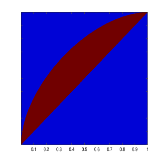
Figure 1: the region $\mathcal{D}$ in the unit cube satisfying (20)

Thanks to the previous theorem we can obtain the following result which shows that $Z$ and $X$ are very similar from a fractal geometry point of view.

Corollary 1

Assume that $a$ and $b$ satisfy (20), then the process $Z$ has the same features $(a)$, $(b)$ and $(c)$ as mBm.

Throughout this article, we use $[x]$ to denote the integer part of a real number $x$. Positive deterministic constants will be numbered as $c_{1},c_{2},\ldots$ while positive random constants will be numbered as $C_{1},C_{2},\ldots$.

2 The main ideas of the proofs

In the reminder of our article we always assume that Condition (20) is satistfied and that $\mbox{diam}({\cal K}):=\sup\{|u-v|:\,(u,v)\in{\cal K}\}\leq 1/4$. Also notice that we will frequently make use of the inequality

$$\log(3+x+y)\leq\log(3+x)\times\log(3+y)\qquad\mathrm{for\;all}\;(x,y)\in\hbox{\it I\hskip-2.0ptR}_{+}^{2}.$$ (22)

Let us now present the main ideas behind the proof of Theorem 1.1. Firstly we need to state the following lemma which allows to conveniently bound the random variables $\varepsilon_{j,k}$. It is a classical result we refer for example to MST (99) or AT (03) for its proof.

Lemma 1

MST (99); AT (03) There are an event $\Omega^{*}$ of probability $1$ and a nonnegative random variable $C_{2}$ of finite moment of every order such the inequality

$$|\varepsilon_{j,k}(\omega)|\leq C_{2}(\omega)\sqrt{\log(3+|j|+|k|)},$$ (23)

holds for all $\omega\in\Omega^{*}$ and $j,k\in\hbox{\it Z\hskip-4.0ptZ}$.

Proof of Theorem 1.1. In view of Remark 1 $(ii)$ and of Remark 2 it is sufficient to prove that Theorem 1.1 holds when the process $R$ is replaced by its high frequency component, namely the process $\ddot{R}=\{\ddot{R}(t):\,\,t\in\hbox{\it I\hskip-2.0ptR}\}$ defined for each $t\in\hbox{\it I\hskip-2.0ptR}$ as

$$\ddot{R}(t)=\ddot{Z}(t)-\ddot{X}(t).$$ (24)

Let $g_{j,k}$ be the function defined on $\hbox{\it I\hskip-2.0ptR}\times\hbox{\it I\hskip-2.0ptR}$ by

$$g_{j,k}(t,\theta)=2^{-j\theta}\Big{\{}\Psi(2^{j}t-k,\theta)-\Psi(-k,\theta)\Big{\}}.$$ (25)

It follows from (24), (15), (18), (25) and (23) that for any $\omega\in\Omega^{*}$,

$$|\ddot{R}(t_{1},\omega)-\ddot{R}(t_{0},\omega)|\leq C_{2}(\omega)\sum_{j=0}^{+\infty}\sum_{k=-\infty}^{+\infty}\sqrt{\log(3+j+|k|)}$$ (26)

$$\hskip 8.5359pt\times\Big{|}g_{j,k}(t_{1},H(k/2^{j}))-g_{j,k}(t_{0},H(k/2^{j}))-g_{j,k}(t_{1},H(t_{1}))+g_{j,k}(t_{0},H(t_{0}))\Big{|}.$$

Next, we expand the term $g_{j,k}\big{(}t_{i},H(\tau)\big{)}$ with $i=0$ or $1$ and $\tau=t_{1}$ or $k/2^{j}$ with respect to the second variable in the neighborhood of $H(t_{0})$. Indeed, since the function $\Psi$ is $\mathcal{C}^{\infty}$, the functions $g_{j,k}$ are also $\mathcal{C}^{\infty}$; thus we can use Taylor-Lagrange Formula of order $1$ with an integral reminder and we get

$$g_{j,k}(t_{1},H(t_{1})) = g_{j,k}(t_{1},H(t_{0}))+(H(t_{1})-H(t_{0}))(\partial_{\theta}g_{j,k})(t_{1},H(t_{0}))$$

$$+(H(t_{1})-H(t_{0}))^{2}\int_{0}^{1}(1-\tau)(\partial_{\theta}^{2}g_{j,k})(t_{1},H(t_{0})+\tau(H(t_{1})-H(t_{0})))\,d\tau,$$

$$g_{j,k}(t_{0},H(k/2^{j})) = g_{j,k}(t_{0},H(t_{0}))+(H(k/2^{j})-H(t_{0}))(\partial_{\theta}g_{j,k})(t_{0},H(t_{0}))$$

$$+(H(k/2^{j})-H(t_{0}))^{2}\int_{0}^{1}(1-\tau)(\partial_{\theta}^{2}g_{j,k})(t_{0},H(t_{0})+\tau(H(k/2^{j})-H(t_{0})))\,d\tau,$$

and

$$g_{j,k}(t_{1},H(k/2^{j})) = g_{j,k}(t_{1},H(t_{0}))+(H(k/2^{j})-H(t_{0}))(\partial_{\theta}g_{j,k})(t_{1},H(t_{0}))$$

$$+(H(k/2^{j})-H(t_{0}))^{2}\int_{0}^{1}(1-\tau)(\partial_{\theta}^{2}g_{j,k})(t_{1},H(t_{0})+\tau(H(k/2^{j})-H(t_{0})))\,d\tau.$$

By adding or subtracting relations (2), (2) and (2) the constant terms disappear and we get the following upper bound

$$\Big{|}g_{j,k}(t_{1},H(k/2^{j}))-g_{j,k}(t_{0},H(k/2^{j}))-g_{j,k}(t_{1},H(t_{1}))+g_{j,k}(t_{0},H(t_{0}))\Big{|}$$ (30)

$$\leq|H(t_{1})-H(t_{0})|\Big{|}(\partial_{\theta}g_{j,k})(t_{1},H(t_{0}))\Big{|}$$

$$+\big{|}H(t_{1})-H(t_{0})\big{|}^{2}\int_{0}^{1}(1-\tau)\Big{|}(\partial_{\theta}^{2}g_{j,k})(t_{1},H(t_{0})+\tau(H(t_{1})-H(t_{0})))\Big{|}\,d\tau$$

$$+|H(k/2^{j})-H(t_{0})|\Big{|}(\partial_{\theta}g_{j,k})(t_{1},H(t_{0}))-(\partial_{\theta}g_{j,k})(t_{0},H(t_{0}))\Big{|}$$

$$+\big{|}H(k/2^{j})-H(t_{0})\big{|}^{2}\int_{0}^{1}(1-\tau)\Big{|}(\partial_{\theta}^{2}g_{j,k})(t_{1},H(t_{0})+\tau(H(k/2^{j})-H(t_{0})))$$

$$\hskip 128.0374pt-(\partial_{\theta}^{2}g_{j,k})(t_{0},H(t_{0})+\tau(H(k/2^{j})-H(t_{0})))\Big{|}\,d\tau.$$

Then, we substitute the previous bound (30) into the inequality (26). We stress that the quantities $|H(t_{1})-H(t_{0})|$ and $\big{|}H(t_{1})-H(t_{0})\big{|}^{2}$ can be factorized outside the sum whereas the quantities $|H(k/2^{j})-H(t_{0})|$ and $\big{|}H(k/2^{j})-H(t_{0})\big{|}^{2}$ remain inside the sum. We obtain

$$|\ddot{R}(t_{1},\omega)-\ddot{R}(t_{0},\omega)| \leq C_{2}(\omega)|H(t_{1})-H(t_{0})|$$

$$\times\Big{\{}\sum_{j=0}^{+\infty}\sum_{k=-\infty}^{+\infty}\sqrt{\log(3+j+|k|)}\times\Big{|}(\partial_{\theta}g_{j,k})(t_{1},H(t_{0}))\Big{|}\Big{\}}$$

$$+\;C_{2}(\omega)|H(t_{1})-H(t_{0})|^{2}\times\Big{\{}\sum_{j=0}^{+\infty}\sum_{k=-\infty}^{+\infty}\sqrt{\log(3+j+|k|)}$$

$$\times\int_{0}^{1}(1-\tau)\Big{|}(\partial_{\theta}^{2}g_{j,k})(t_{1},H(t_{0})+\tau(H(t_{1})-H(t_{0})))\Big{|}\,d\tau\Big{\}}$$

$$+\;C_{2}(\omega)\times\Big{\{}\sum_{j=0}^{+\infty}\sum_{k=-\infty}^{+\infty}\sqrt{\log(3+j+|k|)}|H(k/2^{j})-H(t_{0})|$$

$$\times\Big{|}(\partial_{\theta}g_{j,k})(t_{1},H(t_{0}))-(\partial_{\theta}g_{j,k})(t_{0},H(t_{0}))\Big{|}\Big{\}}$$

$$+\;C_{2}(\omega)\times\Big{\{}\sum_{j=0}^{+\infty}\sum_{k=-\infty}^{+\infty}\sqrt{\log(3+j+|k|)}|H(k/2^{j})-H(t_{0})|^{2}$$

$$\times\int_{0}^{1}(1-\tau)\Big{|}(\partial_{\theta}^{2}g_{j,k})(t_{1},H(t_{0})+\tau(H(k/2^{j})-H(t_{0})))$$

$$\hskip 22.76228pt-(\partial_{\theta}^{2}g_{j,k})(t_{0},H(t_{0})+\tau(H(k/2^{j})-H(t_{0})))\Big{|}\,d\tau\Big{\}}.$$

Then using the following two lemmas whose proofs will be given soon, we get that

$$|\ddot{R}(t_{1},\omega)-\ddot{R}(t_{0},\omega)| \leq C_{2}(\omega)\Big{\{}|H(t_{1})-H(t_{0})|{\cal A}_{1}({\cal K};a,b)+\dots$$

$$+\;\big{|}H(t_{1})-H(t_{0})\big{|}^{2}{\cal A}_{2}({\cal K};a,b)+\dots$$

$$+\;|t_{1}-t_{0}|^{d_{1}}{\cal G}_{1}({\mathcal{K}};a,b,d_{1})+|t_{1}-t_{0}|^{d_{2}}{\cal G}_{2}({\mathcal{K}};a,b,d_{2})\Big{\}}.$$

Finally, in view of (1) the latter inequality implies that Theorem 1.1 holds.  

Lemma 2

For every integer $n\geq 0$ and $(t,\theta)\in\hbox{\it I\hskip-2.0ptR}\times(0,+\infty)$ one sets

$$A_{n}(t,\theta):=\sum_{j=0}^{+\infty}\sum_{k=-\infty}^{+\infty}|(\partial_{\theta}^{n}g_{j,k}(t,\theta)|\sqrt{\log(3+j+|k|)}.$$ (32)

Then one has

$${\cal A}_{n}({\cal K};a,b):=\sup\Big{\{}A_{n}(t,\theta):\,\,(t,\theta)\in{\cal K}\times[a,b]\Big{\}}<\infty.$$ (33)

Lemma 3

For every integer $n\geq 1$ and $(t_{0},t_{1},\theta)\in\hbox{\it I\hskip-2.0ptR}^{2}\times(0,+\infty)$ one sets

$$G_{n}(t_{0},t_{1},\theta) := \sum_{j=0}^{+\infty}\sum_{k=-\infty}^{+\infty}|H(k/2^{j})-H(t_{0})|^{n}\times\sqrt{\log(3+j+|k|)}$$

$$\hskip 42.67912pt\times\Big{|}(\partial_{\theta}^{n}g_{j,k})(2^{j}t_{1}-k,\theta)-(\partial_{\theta}^{n}g_{j,k})(2^{j}t_{0}-k,\theta)\Big{|}.$$

Then, for every integer $n\geq 1$, there is an exponent $d_{n}\in(b,1]$ such that

$${\cal G}_{n}({\mathcal{K}};a,d_{n}):=\sup_{(t_{0},t_{1},\theta)\in{\cal K}^{2}\times[a,b]}|t_{1}-t_{0}|^{-d_{n}}G_{n}(t_{0},t_{1},\theta)<\infty.$$ (34)

Proof of Lemma 2. From Lemma 4 given in next section, one can deduce

$$A_{n}(t,\theta) \leq \sum_{p=0}^{n}C_{n}^{p}|\log 2|^{p}\sum_{j=0}^{+\infty}\sum_{k=-\infty}^{+\infty}j^{p}2^{-j\theta}\sqrt{\log(3+j+|k|)}$$

$$\hskip 85.35826pt\times\Big{\{}\big{|}(\partial_{\theta}^{n-p}\Psi)(2^{j}t-k,\theta)\big{|}+\big{|}(\partial_{\theta}^{n-p}\Psi)(-k,\theta)\big{|}\Big{\}}.$$

Note that the deepest bracket $\displaystyle\Big{\{}\big{|}(\partial_{\theta}^{n-p}\Psi)(2^{j}t-k,\theta)\big{|}+\big{|}(\partial_{\theta}^{n-p}\Psi)(-k,\theta)\big{|}\Big{\}}$ contains two terms: the first $\displaystyle\big{|}(\partial_{\theta}^{n-p}\Psi)(2^{j}t-k,\theta)\big{|}$ depends on $t\in{\cal K}$ whilst the second $\displaystyle\big{|}(\partial_{\theta}^{n-p}\Psi)(-k,\theta)\big{|}$ no longer depends on $t$. Therefore, it suffices to obtain a bound of the supremum for $t\in{\cal K}$ of the sum corresponding to the first term, then to use it in the special case ${\cal K}=\{0\}$ to bound the sum corresponding to the second term. Let us remark that there exists a real $K>0$ such that ${\cal K}\subset[-K,K]$. Thus, without any restriction, we can suppose that ${\cal K}=[-K,K]$. Next, using (8), the convention that $0^{0}=1$, the change of variable $k=k^{\prime}+[2^{j}t]$, the fact that $|t|\leq K$, (22) and the fact that $\displaystyle z=2^{j}t-[2^{j}t]\in[0,1]$ , one has the following estimates for each $p\in\{0,\ldots,n\}$ and $(t,\theta)\in[-K,K]\times[a,b]$:

$$\sum_{j=0}^{+\infty}\sum_{k=-\infty}^{+\infty}j^{p}2^{-j\theta}\,\sqrt{\log(3+j+|k|)}\,\big{|}(\partial_{\theta}^{n-p}\Psi)(2^{j}t-k,\theta)\big{|}$$

$$\leq c_{2}\sum_{j=0}^{+\infty}\sum_{k=-\infty}^{+\infty}j^{p}2^{-ja}\sqrt{\log(3+j+|k|)}\cdot(2+|2^{j}t-k|)^{-\ell}$$

$$\leq c_{2}\sum_{j=0}^{+\infty}\sum_{k^{\prime}=-\infty}^{+\infty}j^{p}2^{-ja}\sqrt{\log(3+j+|k^{\prime}|+2^{j}K)}\cdot(2+|2^{j}t-[2^{j}t]-k^{\prime}|)^{-\ell}$$

$$\leq c_{2}c_{3}\sum_{j=0}^{+\infty}j^{p}2^{-ja}\sqrt{\log(3+j+2^{j}K)}<\infty,$$ (36)

where

$$c_{3}=\sup\Big{\{}\sum_{k=-\infty}^{+\infty}(2+|z-k|)^{-l}\sqrt{\log(3+|k|)}:\,\,z\in[0,1]\Big{\}}<\infty.$$ (37)

Clearly, (2) combined with (2) implies that (33) holds.  

Proof of Lemma 3. The proof is very technical so let us first explain the main ideas behind it. For the sake of simplicity, we make the change of notation $t_{1}=t_{0}+h$. Then we split the set of indices $\{(j,k)\in\hbox{\it I\hskip-2.0ptN}\times\hbox{\it Z\hskip-4.0ptZ}\}$ into three disjoint subsets: ${\cal V}$ a neighborhood of radius $r$ about $t_{0}$, a subset ${\cal W}$ corresponding to the the low frequency ($j\leq j_{1}$) outside the neighborhood ${\cal V}$ and a subset ${\cal W}^{c}$ corresponding to the the high frequency ($j>j_{1}$) outside the neighborhood ${\cal V}$ (the “good” choices of the radius $r$ and of the cutting frequency $j_{1}$ will be clarified soon). Thus the sum through which $G_{n}(t_{0},t_{1},\theta)$ is defined (see the statement of Lemma 3) can be decomposed into three parts: a sum over ${\cal V}$, a sum over ${\cal W}$ and a sum over ${\cal W}^{c}$; they respectively be denoted $B_{1,n}(t_{0},h,\theta)$, $B_{2,n}(t_{0},h,\theta)$ and $B_{3,n}(t_{0},h,\theta)$. In order to be able to show that, to within a constant, each of these three quantities is upper bounded by $|h|^{d_{n}}$ for some exponent $d_{n}>b$, we need to conveniently choose the radius $r$ of the neighborhood ${\cal V}$ as well as the cutting frequency $j_{1}$. The most natural choice is to take $r=|h|$ and $2^{-j_{1}}\simeq|h|$. However a careful inspection of the proof of Lemma 7 shows this does not work basically because $2^{j_{1}}|h|$ does not go to infinity when $|h|$ tends $0$. Roughly speaking, to overcome this difficulty we have taken $r=|h|^{\eta}$ and $2^{-j_{1}}\simeq|h|^{\gamma}$ where $0<\eta<\gamma<1$ are two parameters (the “good” choices of these parameters will be clarified soon) as shown by the following Figure

Fig.2, the three Lemmas and the corresponding subset of indices

More precisely, $j_{1}$ is the unique nonnegative integer satisfying

$$2^{-j_{1}-1}<|h|^{\gamma}\leq 2^{-j_{1}}$$ (38)

and the sets ${\cal V}$, ${\cal W}$ and ${\cal W}^{c}$ are defined by:

$${\cal V}(t_{0},h,\eta)=\{(j,k)\in\hbox{\it I\hskip-2.0ptN}\times\hbox{\it Z\hskip-4.0ptZ}:\,\,|k/2^{j}-t_{0}|\leq|h|^{\eta}\},$$ (39)

$${\cal V}^{c}(t_{0},h,\eta)=\{(j,k)\in\hbox{\it I\hskip-2.0ptN}\times\hbox{\it Z\hskip-4.0ptZ}:\,\,|k/2^{j}-t_{0}|>|h|^{\eta}\},$$ (40)

$${\cal W}(t_{0},h,\eta,\gamma)=\{(j,k)\in{\cal V}^{c}(t_{0},h,\eta):\,\,0\leq j\leq j_{1}\}$$ (41)

and

$${\cal W}^{c}(t_{0},h,\eta,\gamma)=\{(j,k)\in{\cal V}^{c}(t_{0},h,\eta):\,\,j\geq j_{1}+1\}.$$ (42)

It follows from Lemmas 4 to 7 that

$$G_{n}(t_{0},t_{0}+h,\theta)=\sum_{m=1}^{3}B_{m,n}(t_{0},h,\theta)$$

$$\leq\sum_{p=0}^{n}\sum_{m=1}^{3}C_{n}^{p}(\log 2)^{p}B_{m,n,p}(t_{0},h,\theta)$$ (43)

$$\leq c_{4}\Big{(}|h|^{a+\eta\beta}+|h|^{(1-\gamma)+\gamma a}+|h|^{(\gamma-\eta)(\ell-1-\varepsilon)+\gamma a}\Big{)}\log^{n+1/2}(1/|h|),$$

where the constant $c_{4}=\max\{c_{5},c_{8},c_{10}\}\sum_{p=0}^{n}C_{n}^{p}(\log 2)^{p}$ does not depend on $(t_{0},h,\theta)$. In view of (2) and the inequality $\beta>b$ as well as the fact that $\varepsilon$ is arbitrarily small, for proving that (34) holds its sufficient to show that there exist two reals $0<\eta<\gamma<1$ and an integer $l\geq 2$ satisfying the following inequalities

$$\left\{\begin{array}[]{l}a+\eta b\geq b\\ (1-\gamma)+\gamma a\,>b\\ (\gamma-\eta)(\ell-1)+\gamma a\,>\,b.\end{array}\right.$$

This is clearly the case. In fact, thanks to (20) we can easily show that the first two inequalities have common solutions; moreover each of their common solutions is also a solution of the third inequality provided that $\ell$ is big enough.  

Before ending this section let us prove that Corollary 1 holds.

Proof of Corollary 1. Let us first show that $Z$ has the same feature $(b)$ as mBm. In view of Theorem 1.1 and Remark 3 it is clear that $\alpha_{R}$, the pointwise Hölder exponent of $R$, satisfies a.s. for all $t\in\hbox{\it I\hskip-2.0ptR}$,

$$\alpha_{R}(t)\geq d.$$ (44)

Next putting together (44), the fact that $d>b$, (19) and (4) it follows that a.s. for all $t\in\hbox{\it I\hskip-2.0ptR}$,

$$\alpha_{Z}(t)=H(t).$$

Let us now show that $Z$ has the same feature $(c)$ as mBm. Let $(\rho_{n})$ be an arbitrary sequence of positive real numbers converging to $0$. In view of (19) and (6), to prove that for each $t\in\hbox{\it I\hskip-2.0ptR}$ one has

$$\lim_{n\rightarrow\infty}\mbox{law}\left\{\frac{Z(t+\rho_{n}u)-Z(t)}{\rho_{n}^{H(t)}}:\,\,u\in\hbox{\it I\hskip-2.0ptR}\right\}=\mbox{law}\{B_{H(t)}(u):\,\,u\in\hbox{\it I\hskip-2.0ptR}\},$$ (45)

in the sense of finite dimensional distribution, it is sufficient to prove that for any $u\in\hbox{\it I\hskip-2.0ptR}$ one has

$$\lim_{n\rightarrow+\infty}E\left\{\Big{(}\frac{R(t+\rho_{n}u)-R(t)}{\rho_{n}^{H(t)}}\Big{)}^{2}\right\}=0.$$ (46)

Observe that for all $n$ big enough one has $\rho_{n}|u|\leq 1$. Therefore, taking ${\cal K}=[t-1,\,t+1]$ in Theorem 1.1, it follows that for $n$ big enough,

$$E\left\{\Big{(}\frac{R(t+\rho_{n}u)-R(t)}{\rho_{n}^{H(t)}}\Big{)}^{2}\right\}\leq\rho_{n}^{2(d-H(t))}E(C_{1}^{2})$$ (47)

and the latter inequality clearly implies that (46) holds. To have in (45) the convergence in distribution for the topology of the uniform convergence on compact sets it is sufficient to show that for any positive real $L$, the sequence of continuous Gaussian processes,

$$\left\{\frac{Z(t+\rho_{n}u)-Z(t)}{\rho_{n}^{H(t)}}:\,\,u\in[-L,L]\right\},\,n\in\hbox{\it I\hskip-2.0ptN},$$

is tight. This tightness result can be obtained (see B (68)) by proving that there exists a constant $c_{17}>0$ only depending on $L$ and $t$ such that for all $n\in\hbox{\it I\hskip-2.0ptN}$ and each $u_{1},u_{2}\in[-L,L]$ one has

$$E\left\{\Big{(}\frac{Z(t+\rho_{n}u_{1})-Z(t)}{\rho_{n}^{H(t)}}-\frac{Z(t+\rho_{n}u_{2})-Z(t)}{\rho_{n}^{H(t)}}\Big{)}^{2}\right\}\leq c_{17}|u_{1}-u_{2}|^{2H(t)}.$$ (48)

Without loss of generality we may assume that for every $n\in\hbox{\it I\hskip-2.0ptN}$, $\rho_{n}\in(0,1]$. Then by using the fact that (48) is satisfied when $Z$ is replaced by $X$ (see BCI (98) Proposition 2) as well as the fact that it is also satisfied when $Z$ is replaced by $R$ (this can be done similarly to (47)), one can establish that this inequality holds.  

3 Some technical Lemmas

Lemma 4

For every integer $n\geq 0$ and any $(t,\theta)\in\hbox{\it I\hskip-2.0ptR}\times\hbox{\it I\hskip-2.0ptR}$ one has

$$(\partial_{\theta}^{n}g_{j,k})(t,\theta)$$ (49)

$$=\sum_{p=0}^{n}C_{n}^{p}(-j\log 2)^{p}2^{-j\theta}\Big{\{}(\partial_{\theta}^{n-p})\Psi(2^{j}t-k,\theta)-(\partial_{\theta}^{n-p}\Psi)(-k,\theta)\Big{\}}.$$

Proof of Lemma 4. The lemma can easily be obtained by applying the Leibniz formula for the $n$th derivative of a product of two functions.  

Lemma 5

For each integer $n\geq 1$ and $(t_{0},h,\theta)\in\hbox{\it I\hskip-2.0ptR}\times\hbox{\it I\hskip-2.0ptR}\times(0,+\infty)$ set

$$B_{1,n,p}(t_{0},h,\theta) := \sum_{(j,k)\in{\cal V}(t_{0},h,\eta)}j^{p}2^{-j\theta}|H(t_{0})-H(k/2^{j})|^{n}\times\sqrt{\log(3+j+|k|)}$$

$$\hskip 14.22636pt\times\Big{|}(\partial_{\theta}^{n-p}\Psi)(2^{j}(t_{0}+h)-k,\theta)-(\partial_{\theta}^{n-p}\Psi)(2^{j}t_{0}-k,\theta)\Big{|},$$

where ${\cal V}(t_{0},h,\eta)$ is the set defined by (39). Then, for all real $K>0$ and every integers $n\geq 1$ and $0\leq p\leq n$, one has

$$c_{5}:=\sup_{(t_{0},\theta)\in[-K,K]\times[a,b],|h|<1/4}|h|^{-a-n\eta\beta}\log^{-p-1/2}(1/|h|)B_{1,n,p}(t_{0},h,\theta)<\infty.$$

Proof of Lemma 5. It follows from (1) and (39) that

$$\sum_{(j,k)\in{\cal V}(t_{0},h,\eta)}j^{p}2^{-j\theta}|H(t_{0})-H(k/2^{j})|^{n}\times\sqrt{\log(3+j+|k|)}$$ (51)

$$\hskip 85.35826pt\times\Big{|}(\partial_{\theta}^{n-p}\Psi)(2^{j}(t_{0}+h)-k,\theta)-(\partial_{\theta}^{n-p}\Psi)(2^{j}t_{0}-k,\theta)\Big{|}$$

$$\leq c_{1}|h|^{n\beta\eta}\sum_{(j,k)\in{\cal V}(t_{0},h,\eta)}j^{p}2^{-ja}\times\sqrt{\log(3+j+|k|)}$$

$$\hskip 85.35826pt\times\Big{|}(\partial_{\theta}^{n-p}\Psi)(2^{j}(t_{0}+h)-k,\theta)-(\partial_{\theta}^{n-p}\Psi)(2^{j}t_{0}-k,\theta)\Big{|}.$$

Now let $j_{0}\geq 2$ be the unique integer such that

$$2^{-j_{0}-1}<|h|\leq 2^{-j_{0}}.$$ (52)

By using (8), (52), the change of variable $k=k^{\prime}+[2^{j}y]$, (22) and the fact that $|t_{0}|\leq K$, we can deduce that for any $y\in[t_{0}-1,t_{0}+1]$,

$$\sum_{j=j_{0}+1}^{+\infty}\sum_{k=-\infty}^{+\infty}j^{p}2^{-ja}|(\partial_{\theta}^{n-p}\Psi)(2^{j}y-k,\theta)|\sqrt{\log(3+j+|k|)}$$

$$\leq c_{2}\sum_{j=j_{0}+1}^{+\infty}\sum_{k^{\prime}=-\infty}^{+\infty}j^{p}2^{-ja}(2+|2^{j}y-[2^{j}y]-k^{\prime}|)^{-\ell}\sqrt{\log(3+j+2^{j}(|t_{0}|+1)+|k^{\prime}|)}$$

$$\leq c_{2}\cdot c_{3}\sum_{j=j_{0}+1}^{+\infty}j^{p}2^{-ja}\sqrt{\log(3+j+2^{j}(K+1))}$$

$$\leq c_{6}|h|^{a}\log^{p+1/2}(1/|h|),$$ (53)

where $c_{3}$ is the constant defined by (37) and the last inequality (in which $c_{6}$ is a constant non depending on $(t_{0},h,\eta)$) follows from (52) and some classical and easy calculations.

On the other hand, by using the Mean-value Theorem applied to the function $\partial_{\theta}^{n-p}g_{j,k}$ with respect to the first variable, (8), the fact that for all $2^{j}|h|\leq 1$ for all $j\in\{0,\ldots,j_{0}\}$, (52), (22), (37) and the inequality $|t_{0}|\leq K$, we get that

$$\sum_{j=0}^{j_{0}}\sum_{k=-\infty}^{+\infty}j^{p}2^{-ja}\times\sqrt{\log(3+j+|k|)}$$

$$\hskip 85.35826pt\times\Big{|}(\partial_{\theta}^{n-p}\Psi)(2^{j}(t_{0}+h)-k,\theta)-(\partial_{\theta}^{n-p}\Psi)(2^{j}t_{0}-k,\theta)\Big{|}$$

$$\leq c_{2}|h|\sum_{j=0}^{j_{0}}\sum_{k=-\infty}^{+\infty}j^{p}2^{j(1-a)}(1+|2^{j}t_{0}-[2^{j}t_{0}]-k|)^{-\ell}\sqrt{\log(4+j+2^{j}|t_{0}|+|k|)}$$

$$\leq c_{2}c_{3}|h|\sum_{j=0}^{j_{0}}j^{p}2^{j(1-a)}\sqrt{\log(4+j+2^{j}K)}$$

$$\leq c_{7}|h|^{a}\log^{p+1/2}(1/|h|),$$ (54)

where the constant $c_{7}$ does not depend on $(t_{0},h,\eta)$. Finally, by combining (51) with (3) and (3), one can deduce (5).  

Lemma 6

For any $(t,h,\theta)\in\hbox{\it I\hskip-2.0ptR}\times\hbox{\it I\hskip-2.0ptR}\times(0,+\infty)$ and for any integers $n\geq 1$ and $0\leq p\leq n$ set

$$B_{2,n,p}(t_{0},h,\theta) := \sum_{(j,k)\in{\cal W}(t_{0},h,\eta,\gamma)}j^{p}2^{-j\theta}|H(t_{0})-H(k/2^{j})|^{n}\times\sqrt{\log(3+j+|k|)}$$

$$\quad\times\Big{|}(\partial_{\theta}^{n-p}\Psi)(2^{j}(t_{0}+h)-k,\theta)-(\partial_{\theta}^{n-p}\Psi)(2^{j}t_{0}-k,\theta)\Big{|},$$

where ${\cal W}(t_{0},h,\eta,\gamma)$ is the set defined by (41). Then, for any real $K>0$, one has that

$$c_{8} = \sup_{(t_{0},\theta)\in[-K,K]\times[a,b],|h|<1/4}|h|^{-(1-\gamma)-\gamma a}\log^{-p-1/2}(1/|h|)B_{2,n,p}(t_{0},h,\theta)$$ (55)

$$\hskip 256.0748pt<\infty.\hskip 28.45274pt$$

Proof of Lemma 6. To begin with, note that for any pair of real numbers $(\theta_{0},\theta_{1})\in(0,1)^{2}$, one has $|\theta_{1}-\theta_{0}|<1$. Therefore,

$$\mathrm{for\;all}\;(j,k)\in\hbox{\it I\hskip-2.0ptN}\times\hbox{\it Z\hskip-4.0ptZ},\qquad|H(t_{0})-H(k/2^{j})|^{n}<1.$$ (56)

By using the Mean-value Theorem applied to the function $\partial_{\theta}^{n-p}\Psi$ with respect to the first variable combined with (8), we get for all $t_{0}\in\cal K$ and $h\in\hbox{\it I\hskip-2.0ptR}$

$$\Big{|}(\partial_{\theta}^{n-p}\Psi)(2^{j}(t_{0}+h)-k,\theta)-(\partial_{\theta}^{n-p}\Psi)(2^{j}t_{0}-k,\theta)\Big{|}\hskip 85.35826pt$$

$$\leq c_{2}\,2^{j}|h|\,\big{(}2+|2^{j}t_{0}-k+2^{j}uh|\big{)}^{-\ell}$$

for a real number $u\in(0,1)$. On the other hand it follows the inequality $2^{j}|h|\leq 1$ for all $j\in\{0,\ldots,j_{1}\}$ (which is a consequence of (38)) and from triangle inequality that $|2^{j}t_{0}-k+2^{j}uh|\geq|2^{j}t_{0}-k|-1$. Therefore

$$\Big{|}(\partial_{\theta}^{n-p}\Psi)(2^{j}(t_{0}+h)-k,\theta)-(\partial_{\theta}^{n-p}\Psi)(2^{j}t_{0}-k,\theta)\Big{|}\hskip 85.35826pt$$

$$\leq c_{2}\,2^{j}|h|\,\big{(}1+|2^{j}t_{0}-k|\big{)}^{-\ell}$$

and as a consequence, we obtain for all $(t,h,\theta)\in\hbox{\it I\hskip-2.0ptR}\times\hbox{\it I\hskip-2.0ptR}\times(0,1)$

$$B_{2,n,p}(t_{0},h,\theta) \leq c_{2}|h|\sum_{j=0}^{j_{1}}\sum_{k=-\infty}^{+\infty}j^{p}\,2^{j(1-\theta)}(1+|2^{j}t_{0}-k|)^{-\ell}\sqrt{\log(3+j+|k|)}.$$

Next, making the change of variable $k=k^{\prime}+[2^{j}t_{0}]$ and using triangle inequality as well as the inequality $\theta\geq a$, we deduce that for all $(t,h,\theta)\in[-K,K]\times[-1/4,1/4]\times[a,b]$

$$B_{2,n,p}(t_{0},h,\theta) \leq c_{2}|h|\sum_{j=0}^{j_{1}}\sum_{k^{\prime}=-\infty}^{+\infty}j^{p}2^{j(1-a)}(1+|2^{j}t_{0}-[2^{j}t_{0}]-k^{\prime}|)^{-\ell}$$

$$\hskip 142.26378pt\times\sqrt{\log(3+j+2^{j}|t_{0}|+|k^{\prime}|)}$$

$$\leq c_{2}|h|\left\{\sum_{k^{\prime}=-\infty}^{+\infty}\sqrt{\log(3+|k^{\prime}|)}(1+|2^{j}t_{0}-[2^{j}t_{0}]-k^{\prime}|)^{-\ell}\right\}$$

$$\hskip 14.22636pt\times\left\{\sum_{j=0}^{j_{1}}j^{p}2^{j(1-a)}\sqrt{\log(4+j+2^{j}K|)}\right\},$$

where the last inequality follows from $|t_{0}|\leq K$ and the inequality (22). Set $z=2^{j}t_{0}-[2^{j}t_{0}]$, obviously $z\in[0,1)$, thus (37) and the latter inequality imply that

$$B_{2,n,p}(t_{0},h,\theta) \leq c_{2}\cdot c_{3}\,|h|\,\left\{\sum_{j=0}^{j_{1}}j^{p}2^{j(1-a)}\sqrt{\log(4+j+2^{j}K|)}\right\},$$

for all $(t,h,\theta)\in[-K,K]\times[-1/4,1/4]\times[a,b]$. Finally, in view of the inequalities $2^{j_{1}}\leq|h|^{-\gamma}$ and $j_{1}\leq\log(1/|h|)$ (these inequalities are a consequences of (38)), we get

$$B_{2,n,p}(t_{0},h,\theta)\leq c_{9}|h|^{(1-\gamma)+\gamma a}\log^{p+1/2}(1/|h|),$$ (57)

where the constant $c_{9}$ does not depend on $(t_{0},h,\theta)$. This finishes the proof of Lemma 6.  

Lemma 7

For any $(t,h,\theta)\in\hbox{\it I\hskip-2.0ptR}\times\hbox{\it I\hskip-2.0ptR}\times[a,b]$ and any integers $n\geq 1$ and $0\leq p\leq n$ set

$$B_{3,n,p}(t_{0},h,\theta) := \sum_{(j,k)\in{\cal W}^{c}(t_{0},h,\eta,\gamma)}j^{p}2^{-j\theta}|H(t_{0})-H(k/2^{j})|^{n}\times\sqrt{\log(3+j+|k|)}$$

$$\quad\times\Big{|}(\partial_{\theta}^{n-p}\Psi)(2^{j}(t_{0}+h)-k,\theta)-(\partial_{\theta}^{n-p}\Psi)(2^{j}t_{0}-k,\theta)\Big{|}$$

where ${\cal W}^{c}(t_{0},h,\eta,\gamma)$ is the set defined by (42). Then, for every real $K>0$, for each arbitrarily small real $\varepsilon>0$ and all integer $l\geq 2$, one has $c_{10}<\infty$ where

$$c_{10} := \sup_{(t_{0},\theta)\in[-K,K]\times[a,b],|h|<1/4}|h|^{-(\gamma-\eta)(l-1-\varepsilon)-\gamma a}\log^{-p-1/2}(|h|^{-1})B_{2,n,p}(t_{0},h,\theta)$$

Proof of Lemma 7. By using the triangle inequality combined with (42) and (40), one gets, for all $(j,k)\in{\cal W}^{c}(t_{0},h,\eta,\gamma)$,

$$|(t_{0}+h)-k2^{-j}| \geq |t_{0}-k2^{-j}+h|\geq|h|^{\eta}-|h|\geq c_{11}|h|^{\eta},$$ (58)

where the constant $c_{11}=1-4^{\eta-1}$. This means that the integer $k$ necessarily satisfies

$$|2^{j}(t_{0}+h)-k|\geq c_{11}2^{j}|h|^{\eta}.$$ (59)

In view of (59), let us consider ${\cal T}_{j}^{+}$ and ${\cal T}_{j}^{-}$ the sets of positive real numbers defined by

$${\cal T}_{j}^{+}=\{|2^{j}(t_{0}+h)-k|:\,\,\mbox{ $k\in\hbox{\it Z\hskip-4.0ptZ}$ and $2^{j}(t_{0}+h)-k\geq c_{11}2^{j}|h|^{\eta}$}\}$$

and

$${\cal T}_{j}^{-}=\{|2^{j}(t_{0}+h)-k|:\,\,\mbox{ $k\in\hbox{\it Z\hskip-4.0ptZ}$ and $k-2^{j}(t_{0}+h)\geq c_{11}2^{j}|h|^{\eta}$)}\}.$$

For every fixed $j$, the set ${\cal T}_{j}^{+}$ can be viewed as a strictly increasing sequence $(\tau_{j,q}^{+})_{q\in\hbox{\it I\hskip-2.0ptN}}$ satisfying for all $q\in\hbox{\it I\hskip-2.0ptN}$,

$$q+c_{11}2^{j}|h|^{\eta}\leq\tau_{j,q}^{+}<q+1+c_{11}2^{j}|h|^{\eta}.$$ (60)

Similarly, for every fixed $j$, the set ${\cal T}_{j}^{-}$ can be viewed as a strictly increasing sequence $(\tau_{j,q}^{-})_{q\in\hbox{\it I\hskip-2.0ptN}}$ satisfying for all $q\in\hbox{\it I\hskip-2.0ptN}$,

$$q+c_{11}2^{j}|h|^{\eta}\leq\tau_{j,q}^{-}<q+1+c_{11}2^{j}|h|^{\eta}.$$ (61)

Next, setting ${\cal T}_{j}={\cal T}_{j}^{+}\cup{\cal T}_{j}^{-}$, it follows that from (8), the triangle inequality, the inequality $|t_{0}+h|\leq K+1$, (42), (59), (60) and (61) that

$$\sum_{(j,k)\in{\cal W}^{c}(t_{0},h,\eta,\gamma)}j^{p}2^{-j\theta}\Big{|}(\partial_{\theta}^{n-p}\Psi)(2^{j}(t_{0}+h)-k,\theta)\Big{|}\sqrt{\log(3+j+|k|)}$$

$$\leq c_{2}\sum_{(j,k)\in{\cal W}^{c}(t_{0},h,\eta,\gamma)}j^{p}2^{-j\theta}\Big{(}2+|2^{j}(t_{0}+h)-k|\Big{)}^{-\ell}\times\dots$$

$$\hskip 113.81102pt\times\sqrt{\log(3+j+|2^{j}(t_{0}+h)-k|+2^{j}(K+1))}$$

$$\leq c_{2}\sum_{j=j_{1}+1}^{+\infty}\sum_{\tau\in{\cal T}_{j}}j^{p}2^{-j\theta}\Big{(}2+|\tau|\Big{)}^{-\ell}\sqrt{\log(3+j+|\tau|+2^{j}(K+1))}$$

$$\leq 2c_{2}\sum_{j=j_{1}+1}^{+\infty}\sum_{q=0}^{+\infty}j^{p}2^{-ja}\Big{(}2+q+c_{11}2^{j}|h|^{\eta}\Big{)}^{-\ell}\times\dots$$

$$\hskip 113.81102pt\times\sqrt{\log(4+j+q+2^{j}|h|^{\eta}+2^{j}(K+1))}$$

Then, one can use the inequality $\displaystyle(2+x)^{-\ell}\sqrt{\log(4+x)}\leq c_{12}(2+x)^{-\ell+\varepsilon}$ which is valid for all nonnegative real number $x$ where $\varepsilon$ is a fixed arbitrarily small positive real number and $c_{12}$ is a constant only depending on $\varepsilon$. By combining this inequality with (22), (38) and $|h|\leq 1/4$, we get

$$\sum_{(j,k)\in{\cal W}^{c}(t_{0},h,\eta,\gamma)}j^{p}2^{-j\theta}\Big{|}(\partial_{\theta}^{n-p}\Psi)(2^{j}(t_{0}+h)-k,\theta)\Big{|}\sqrt{\log(3+j+|k|)}$$

$$\leq 2c_{2}\sum_{j=j_{1}+1}^{+\infty}\sum_{q=0}^{+\infty}j^{p}2^{-ja}\sqrt{\log(3+j+2^{j}(K+1))}\times\dots$$

$$\hskip 56.9055pt\times\Big{(}2+q+c_{11}2^{j}|h|^{\eta}\Big{)}^{-\ell}\sqrt{\log(4+q+c_{11}2^{j}|h|^{\eta})}$$

$$\leq 2c_{2}c_{12}\sum_{j=j_{1}+1}^{+\infty}j^{p}2^{-ja}\sqrt{\log(3+j+2^{j}(K+1))}\times\dots$$

$$\hskip 142.26378pt\times\left(\int_{0}^{+\infty}\Big{(}1+y+c_{11}2^{j}|h|^{\eta}\Big{)}^{-\ell+\varepsilon}dy\right)$$

$$\leq c_{13}\sum_{j=j_{1}+1}^{+\infty}j^{p}2^{-ja}\sqrt{\log(3+j+2^{j}(K+1)))}\Big{(}1+c_{11}2^{j}|h|^{\eta}\Big{)}^{-(\ell-1-\varepsilon)}$$

$$\leq c_{14}|h|^{-\eta(\ell-1-\varepsilon)}\sum_{j=j_{1}+1}^{+\infty}j^{p}2^{-j(a+\ell-1-\varepsilon)}\sqrt{\log(3+j+2^{j}(K+1))}$$

$$\leq c_{15}\,|h|^{(\gamma-\eta)(\ell-1-\varepsilon)+\gamma a}\log^{p+1/2}(1/|h|),$$

where $c_{12}$, $c_{13}$, $c_{14}$ and $c_{15}$ are constants which do not depend on $(t_{0},h,\theta)$. Finally, using the latter inequality as well as the triangle inequality and the fact that $H(\cdot)$ is with values in $[a,b]$ we get the lemma.  

Acknowledgments. The authors thank the anonymous referee for many useful remarks which greatly helped them to improve the earlier version of this article.

References

ABLV (07) Ayache, A., Bertrand, P. R., Lévy Véhel, J.: A central limit theorem for the generalized quadratic variation of the step fractional Brownian motion. Stat. Inference Stoch. Process., 10, 1, 1–27 (2007)
AT (03) Ayache, A., Taqqu, M.S.: Rate optimality of wavelet series approximations of fractional Brownian motion. J. Fourier Anal. Appl., 9(5), 451–471 (2003)
AT (05) Ayache, A., Taqqu, M.S.: Multifractional process with random exponent. Publ. Mat., 49, 459–486 (2005)
AJT (07) Ayache, A., Jaffard, S., Taqqu M.S.: Wavelet construction of generalized multifractional processes. Rev. Mat. Iberoamericana., 23, 1, 327–370 (2007)
BBCI (00) Benassi, A., Bertrand, P. R., Cohen, S., Istas, J.: Identification of the Hurst index of a step fractional Brownian motion. Stat. Inference Stoch. Proc., 3, 1/2, 101–111 (2000)
BCI (98) Benassi, A., Cohen, S., Istas, J.: Identifying the multifractional function of a Gaussian process. Stat. Probab. Letters., 39, 337–345 (1998)
B (68) Billingsley, P.: Convergence of Probability Measures. John Wiley & Sons (1968)
C (99) Cohen, S.: From self-similarity to local self-similarity: the estimation problem. Fractals: Theory and Applications in Engineering, Springer, eds Dekind, Lévy Véhel, Lutton and Tricot 3–16 (1999)
F (02) Falconer, K.J.: Tangent fields and the local structure of random fields. J. Theoret. Probab., 15, 731–750 (2002)
F (03) Falconer, K.J.: The local structure of random processes. J. London Math. Soc.(2) 67, 657–672 (2003)
(12) Falconer, K.J., Lévy Véhel, J.: Localisable moving
average stable and multistable processes. To appear in J. Theoret. Probab.