Occupation Statistics of a BEC for a Driven Landau-Zener Crossing

Abstract

We consider an atomic Bose-Einstein condensate (BEC) loaded in a biased double-well trap with tunneling rate $K$ and interatomic interaction $U$. The BEC is prepared such that all $N$ atoms are in the left well. We drive the system by sweeping the potential difference $\mathcal{E}$ between the two wells. Depending on the interaction $u=NU/K$ and the sweep rate $\dot{\mathcal{E}}$, we distinguish three dynamical regimes: adiabatic, diabatic, and sudden and consider the occupation statistics of the final state. The analysis goes beyond mean-field theory and is complemented by a semiclassical picture.

The theoretical and experimental study of driven atomic Bose-Einstein Condensates (BEC) in a few site system using optical lattice technology has intensified in recent years AGFHGO05 ; CSMHPR05 ; FTCFSWMB07 ; CTFSMFB08 . Beyond the fundamental interest of these studies, they also aim to create a new generation of nanoscale devices such as atom transistors SAZ07 . Consequently, a wealth of research has been done on the prototype two-site (dimer) system, either within the framework of a nonlinear mean-field approach AGFHGO05 , optionally using higher order cumulants AV01 , or adopting a conventional many-body perspective KBK03 ; TWK08 ; HKO06 ; GKN08 . Such investigations have revealed many interesting phenomena associated with eigenvalue spectra, the structure of the eigenstates, wave-packet dynamics, e.g. of the Bloch-Josephson type, and leaking dynamics due to dissipative edges.

Driven dimers prove to be even more challenging WN00 ; LFOCN02 ; WGK06 ; SRM08 ; AG08 . The scenario investigated in these studies involves many-body Landau-Zener (LZ) transitions induced by sweeping the potential difference $\mathcal{E}$ between the two wells. Specifically, one assumes that initially $\mathcal{E}$ is very negative and that all $n=N$ atoms are in the first well. Then $\mathcal{E}$ is increased at some constant rate $\dot{\mathcal{E}}$ to a very positive value. The objective is to calculate how many atoms ($n$) remain in the first well. The majority of published works are based on the Gross-Pitaevskii equation (or its discrete analogue), which is a mean-field approach WN00 ; LFOCN02 . There are only a few studies that have made further progress within the framework of a full quantum mechanical treatment of the system WGK06 ; SRM08 ; AG08 . However, they all focus on calculating the average occupation $\langle n\rangle$, neglecting to form a theory for the occupation statistics $P(n)$ and, in particular, for the variance $\mbox{Var}(n)$.

Outline. – In this Letter, we consider a driven dimer with intersite hopping amplitude $K$ and interatomic interaction $U$. The parameter $u=NU/K$ can be either positive (repulsive) or negative (attractive) and its magnitude determines various dynamical regimes itemB4 : Rabi (${|u|<1}$), Josephson (${1<|u|<N^{2}}$), or Fock (${|u|>N^{2}}$). Depending on the sweep rate $\dot{\mathcal{E}}$ we distinguish between adiabatic, diabatic, and sudden dynamical scenarios and study the asymptotic occupation statistics as a function of $u$. Our analysis goes beyond mean-field theory, using a semiclassical picture and involving detailed simulations.

Modeling. – The simplest model that describes interacting bosons on a lattice is the Bose-Hubbard Hamiltonian (BHH), which in case of the dimer (two sites) reads:

$$\mathcal{H}\!=\!\sum_{i=1}^{2}\!\left[\mathcal{E}_{i}{\hat{n}}_{i}+\frac{U}{2}{\hat{n}}_{i}({\hat{n}}_{i}-1)\right]\!-\!\frac{K}{2}\sum_{i\neq j}\hat{b}_{i}^{\dagger}\hat{b}_{j}$$ (1)

with $\hbar{=}1$, where $\hat{b}_{i}$ and $\hat{b}_{i}^{\dagger}$ are bosonic annihilation and creation operators and ${\hat{n}}_{i}=\hat{b}_{i}^{\dagger}\hat{b}_{i}$ counts the number of particles at site ${i=1,2}$. The validity of this two-mode approximation itemA8a for a double well is discussed in Refs. itemA8b ; itemA8c , as well as in Ref. itemC1b for biased systems, and it was found to yield good agreement with the experiment itemB4 . The total number of particles $N=\hat{n}_{1}+\hat{n}_{2}$ is a constant of motion, allowing us to consider a Hilbert-space of dimension ${{\cal N}=N{+}1}$, which is spanned by the Fock basis states ${|n\rangle\equiv|n_{1}{=}n,n_{2}{=}N{-}n\rangle}$. Below we assume an even $N\gg 1$ and define ${j=N/2}$, hence ${{\cal N}=2j{+}1}$. The BHH for a given $N$ is formally equivalent to the Hamiltonian of a spin $j$ particle. Defining ${J_{z}\equiv({\hat{n}}_{1}-{\hat{n}}_{2})/2}$ and ${J_{+}\equiv\hat{b}_{1}^{\dagger}\hat{b}_{2}}$ it can be rewritten as:

$$\hat{H}=U{\hat{J}}_{z}^{2}+\mathcal{E}{\hat{J}}_{z}-K{\hat{J}}_{x};\quad\mathcal{E}=\mathcal{E}_{1}-\mathcal{E}_{2}$$ (2)

where $\mathcal{E}$ is the bias. In the absence of interaction, this Hamiltonian can be reinterpreted as describing a spin in a magnetic field with precession frequency ${\Omega=(-K,0,\mathcal{E})}$.

The many-body Landau-Zener scenario assumes that initially all particles are located in the first site ${|\Psi(t{=}0)\rangle=|N\rangle}$. The bias $\mathcal{E}$ is then varied with some constant sweep rate $\dot{\mathcal{E}}$. At the end of the sweep the occupation statistics $P(n)\equiv|\langle n|\Psi(t)\rangle|^{2}$ becomes time-independent. Depending on the outcome (Fig. 1) we distinguish between: (i) an adiabatic process ${P(n)\approx\delta_{n,0}}$; (ii) a sudden process ${P(n)\approx\delta_{n,N}}$; and (iii) a diabatic process ${P(n)\approx\delta_{n,n_{c}}}$, where ${n_{c}\neq 0,N}$.

Phase Space. – In order to analyze the dynamics for finite $U$, it is convenient to rewrite the BHH using canonical variables. Formally, our system corresponds to two coupled oscillators and thus we can define action-angle variables ${\hat{b}}_{i}\equiv\sqrt{{\hat{n}}_{i}}\exp(i\varphi_{i})$. Note that the translation-like operator $\exp(i\varphi)$ is in fact non-unitary because it annihilates the ground state, but this is irrelevant for ${N\gg 1}$ itemB4 ; itemB3 . With these coordinates the BHH takes a form that resembles the Josephson Hamiltonian:

$$\mathcal{H}\ \approx\ \frac{NK}{2}\left[\frac{1}{2}u(\cos\theta)^{2}+\varepsilon\cos\theta-\sin\theta\cos\varphi\right],$$ (3)

where $\theta$ is an alternative way to express the occupation difference ${J_{z}\equiv(\hat{n}_{1}{-}\hat{n}_{2})/2\equiv(N/2)\cos(\theta)}$ and ${\varphi\equiv\varphi_{1}{-}\varphi_{2}}$. The scaled bias is $\varepsilon\equiv\mathcal{E}/K$. Note that $\varphi$ and $\theta$ do not commute. The classical phase space is described either using the canonical coordinates ${(\varphi,\mathsf{n})}$, with ${\mathsf{n}\equiv J_{z}{+}(N/2)\in[0,N]}$, or equivalently using the spherical coordinates ${(\varphi,\theta)}$. In the former case the total area of phase space is $2\pi N$ with a Planck cell ${2\pi\hbar}$ and $\hbar{=}1$, while in the latter case the phase space has total area $4\pi$ with a Planck cell ${4\pi/N}$. Within the semiclassical approximation, a quantum state is described as a distribution in phase space and the eigenstates are associated with stripes that are stretched along contour lines ${\mathcal{H}(\varphi,\theta)=E}$. The energy levels $E_{n}$ can be determined via WKB quantization of the enclosed phase space area.

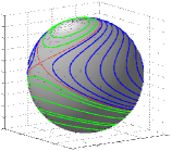
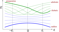
Figure 1: (Color online) Phase space and corresponding energy levels (conceptual plot). Note that a ground state preparation of a ${U<0}$ system with increasing bias $\mathcal{E}(t)$ is equivalent to a preparation in the most excited state of a $U>0$ system with decreasing bias. The latter convention has been adopted in the right panel and in our simulations.

Separatrix. – The phase space topology becomes non-trivial, i.e. has more than one component as in Fig. 1a, if ${|u|>1}$ and $|\varepsilon|<\varepsilon_{c}$ where ${\varepsilon_{c}=(u^{2/3}-1)^{3/2}}$. In this regime, a separatrix divides the phase space into three regions: two islands (green) that contain the upper energy levels and a sea (blue) that contains the lower energy levels. In this description and in the numerics below we assume $U>0$ and adopt the following enumeration convention: we define $E_{0}$ as the most excited level, while $E_{N}$ corresponds to the lowest one. Note that the replacement $U\mapsto-U$ would merely invert the order of the levels, and $E_{0}$ would become the ground state.

Fig. 1b is an illustration of the energy levels as a function of the bias. Each level is associated via WKB quantization with one of the contour lines in Fig. 1a. For the sake of our later analysis we define $E_{n_{c}}$ as the level which is closest to the separatrix for $|\varepsilon|=\varepsilon_{c}$. At this critical value of the bias one of the islands has a vanishing phase space area, while the area of the other is ${A_{c}\approx 4\pi\varepsilon_{c}/u}$. Using WKB quantization we get

$$n_{c}\ \ =\ \ \frac{A_{c}}{4\pi/N}\ \ \approx\ \ (1-u^{-2/3})^{3/2}\ N,$$ (4)

where the approximation for $A_{c}$ has been derived using methods as in Ref.LFOCN02 , and has been tested numerically.

(a)                  (b)                      (c)

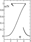
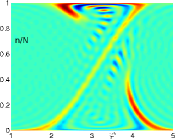
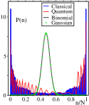
Figure 2: (Color online) Dynamical evolution in a situation in which the mean-field (Gaussian) approximation does not hold: $N{=}100$ particles are prepared in one site of a symmetric ($\mathcal{E}{=}0$) double well and then evolved with a $u{=}2$ Hamiltonian. The initial wave-packet is stretched along the separatrix. (a) (semi)classical distribution in phase space. (b) Wigner function of the corresponding quantum state. (c) Quantum $P(n)$ compared with the (semi)classical and with the mean-field (binomial/Gaussian) predictions. The average occupation $\langle n\rangle{=}47$ is associated here with a huge super-binomial variance $\mbox{Var}(n){=}1530$ instead of the binomial value $\mbox{Var}(n){\sim}25$. In all the simulations we use a 4th order Runge-Kutta and made sure that during the integration the probability leakage is $\ll 10^{-6}$.

Simulations. – As a preliminary step we did simulations of the undriven wave-packet dynamics with $\mathcal{E}{=}0$ and $u{=}2$. For this value of $u$ the separatrix crosses the north pole of the phase space and therefore the wave-packet stretches along it, as illustrated in Fig. 2a (classical) and in Fig. 2b (quantum mechanical). We note that this type of dynamics cannot be properly addressed by the mean-field approximation. The mean-field equation merely describes the Hamiltonian evolution of a single point in phase space and therefore assumes that the wave-packet looks like a minimal Gaussian at any moment. Whenever the motion takes place near the separatrix, the mean-field description becomes inapplicable and consequently the distribution $P(n)$ is likely not to be binomial (Fig. 2c). In what follows we use the terms sub/super-binomial in order to refer to a $P(n)$ with a smaller/larger spreading than the mean-field results. For the dynamics described in Fig. 2, the stretching along the separatrix leads to a super-binomial result.

Next, we address the effect of separatrix motion on $P(n)$ in the bias-sweep scenario. Note that this separatrix motion cannot be avoided: For ${\varepsilon<-\varepsilon_{c}}$ the wave-packet is localized in the upper level. When ${\varepsilon=-\varepsilon_{c}}$ the separatrix emerges. As long as ${-\varepsilon_{c}<\varepsilon<0}$ the wave-packet remains trapped in the top of the big island which gradually shrinks. When $\varepsilon$ becomes larger than zero, the wave-packet can partially tunnel out from the shrinking island to the levels of the expanding island. When ${\varepsilon=+\varepsilon_{c}}$, the shrinking island disappears and the remaining part of the wave-packet is squeezed out along the $n=n_{c}$ contour, resembling the dynamics of Fig. 2. One observes that the stretching along the separatrix during the nonlinear LZ transition is accompanied by narrowing in the transverse direction. This leads to a sub-binomial rather than super-binomial result for the distribution $P(n)$ at the end of the sweep.

In Fig. 3 we plot the average occupation $\langle n\rangle$ and the participation number PN$\equiv[{\sum_{n}P(n)^{2}}]^{-1}$ of the distribution at the end of the sweep as a function of $\dot{\varepsilon}$. These, unlike $\langle n\rangle$, provides significantly more information regarding the nature of the crossing process. For very slow rates, the wave-packet follows a strict adiabatic process ending in $n{=}0$, i.e. all particles move to the other site. For a moderate sweep rate the wave-packet ends in a superposition of $n{=}0$ and $n{=}1$ states, indicated by PN${=}2$. We also resolve the possibility of ending entirely at $n{=}1$ or at $n{=}2$ or at $n{=}3$. In the case shown in Fig. 3, we have ${n_{c}\approx 4}$. For larger sweep rates, we observe a qualitatively different behavior that can be described as a crossover from an adiabatic/diabatic behavior to a sudden behavior at the peak value PN${=}4$. In order to appreciate the deviation of the numerical results from the mean-field theory prediction, we plot $\mbox{Var}(n)$ versus $\langle n\rangle$ in Fig. 4 and compare with the binomial expectation. We further analyze the observed results in the last section.

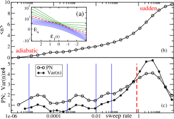
Figure 3: (Color online) (a) Parametric evolution of the adiabatic energy levels versus the decreasing $\mathcal{E}_{1}(t)$ for $N{=}10$ particles and $u{=}2.5$. We use units of time such that $K{=}1$. The dashed line corresponds to the level $n_{c}{=}4$. (b) Average occupation $\langle n\rangle$ versus the sweep rate $\dot{\mathcal{E}}$. (c) Participation number (PN) and $\mbox{Var}(n)$ versus $\dot{\mathcal{E}}$. The vertical lines indicate the various adiabatic and diabatic (dashed) thresholds.

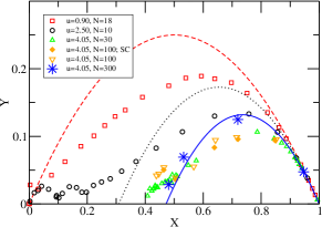
Figure 4: (Color online) $Y=\mbox{Var}(n)/N$ versus $X=\langle n\rangle/N$. Symbols correspond to numerical data, while lines indicate the sub-binomial scaling relation Eq.(6) with $u{=}2.5$ (dotted) and $u{=}4.05$ (solid). No fitting is involved. As a reference we plot the standard binomial scaling (dashed line) which would strictly apply in the absence of interaction ($u{=}0$), and the results of semiclassical (SC) simulations which are obtained by running ensemble of trajectories in phase space. There is a clear crossover from a binomial to the sub-binomial scaling and the agreement becomes better for large $N$. Note that the super-binomial data point ${(X,Y)=(0.47,15.3)}$ that corresponds to the distribution in Fig. 2 is out-of-scale.

Thresholds. – The various thresholds that are involved in the adiabatic-diabatic-sudden crossovers are indicated in Fig. 5. They all follow from the breakdown of a “slowness condition” that can be written as

$$\dot{\mathcal{E}}\ \ \ll\ \ \omega_{\mbox{\tiny osc}}^{2}\ /\ \kappa,$$ (5)

where $\omega_{\mbox{\tiny osc}}$ is a characteristic frequency of the unperturbed dynamics and $\kappa$ is the coupling parameter that determines the rate of the driven transitions.

In the strict quantum adiabatic framework, $\omega_{\mbox{\tiny osc}}$ is simply the level spacing and $\kappa$ is determined by the slopes of the intersecting levels. In order to determine the adiabatic thresholds in Fig. 3 we observe that for the intersection of the $0$th level with the $(N{-}n)$ level the difference in slope is $\kappa=(N{-}n)$, because asymptotically ${d(E_{n}{-}E_{m})/d\mathcal{E}\sim(n{-}m)}$. In the absence of interaction ($u\ll 1$), the level spacing is $\omega_{\mbox{\tiny osc}}=K$ and only nearby levels are coupled, leading to the standard Landau-Zener adiabaticity condition ${\dot{\mathcal{E}}\ll K^{2}}$. With strong interaction there is an $N$th order coupling between the $n{=}0$ level and the $n{=}N$ level, which allows tunneling from the top of one island to the top of the other island (as illustrated in Fig. 1). An estimate for this coupling is $K_{\mbox{\tiny eff}}=[NK]/[2^{N{-}1}(N{-}1)!](K/U)^{N{-}1}$ KBK03 . Similar considerations can be applied to the bottom sea level leading to the distinction between mega, gradual, and sequential crossings (see Ref.HKC08 ).

For large $N$ it might be practically impossible to satisfy the strict adiabatic condition which is associated with the possibility to tunnel from the top of one island to the top of the other. Then the relevant mechanism for transition, i.e. the emission to the level $n_{c}$ as described in the previous section, becomes semiclassical. The frequency that governs this process is the oscillation frequency at the bottom of the sea ${\omega_{\rm osc}\sim|NUK|^{1/2}}$. It determines the level spacing of the lower energy levels and also describes the level spacing in the vicinity of the separatrix, apart from some logarithmic corrections csp . It follows that the diabatic-sudden crossover involves the threshold condition ${\dot{\mathcal{E}}\ll|NUK|}$ as indicated in Fig. 5 and in Fig. 3 for the specific parameters of the simulations.

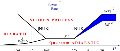
Figure 5: (Color online) Diagram of the $(U,\dot{\mathcal{E}})$ regimes for a ground state preparation. In the Rabi regime $|U|<K/N$ we have a crossover from adiabatic to sudden behavior. For ${K/N<U<NK}$ (or ${U>NK}$) we have a broad crossover from adiabatic gradual (or sequential HKC08 ) behavior to sudden behavior. For ${U<-K/N}$ we have two crossovers: the first from quantum adiabatic to diabatic behavior and the second from diabatic to sudden behavior. The diabatic behavior can be regarded as a classical nonlinear adiabatic behavior. For ${U<-NK}$ the distinction between the diabatic and the sudden regime is blurred because the final state is the same.

Scaling. – Due to the squeezing along the separatrix, the spreading of the wavepacket for an idealized diabatic process becomes negligible in the transverse direction. The diabatic-sudden crossover is related to the non-adiabatic transitions between the remaining $(N{-}n_{c})$ sea levels, where nonlinear effects are negligible. It follows that the spreading can be approximately modeled by the toy Hamiltonian $\mathcal{H}=h(t)\cdot J$, where $J$ is a spin entity with $j_{\mbox{\tiny eff}}=(N{-}n_{c})/2$, and $h(t)$ is a field with constant magnitude $|h(t)|=\omega_{\mbox{\tiny osc}}$ corresponding to the mean-level spacing. The sweep is like a rotation of $h(t)$ in the plane with some angular rate $\omega$. For such a (linear) model the mean-field approximation is exact and therefore we suggest (due to the truncation of Hilbert space) a sub-binomial rather than binomial scaling relation between the mean and the variance of the occupation statistics:

$$Y\ =\ (1-X)\frac{X-c}{1-c};\quad{\rm with}\quad c=\frac{n_{c}}{N},$$ (6)

where ${X=\langle n\rangle/N}$ and ${Y=\mbox{Var}(N)/N}$. Our numerical data is reported in Fig. 4 together with the binomial ($c{=}0$) and sub-binomial scaling relation Eq.(6). The numerics confirm the expected $u$-dependent crossover from binomial to sub-binomial statistics, where the latter, with no fitting parameters, sets a lower bound for the variance.

Summary. – In view of the strong research interest in counting statistics of electrons in mesoscopic devices, it is surprising that the issue of occupation statistics of BECs has been explored only for equilibrium phase transitions. We were motivated to address this subject in the framework of dynamical processes by state-of-the-art experiments aimed at counting individual particles CSMHPR05 ; FTCFSWMB07 ; CTFSMFB08 . We have shown that in the case of a many-body Landau-Zener transition the mean-field binomial expectation is not realized, however a sub-binomial scaling relation still works quite well. The study of the occupation statistics and, in particular, the participation number of the final distribution, allowed us to resolve all the details of the adiabatic-diabatic-sudden crossovers and to verify theoretical estimates for the threshold of each crossover.

Acknowledgments. – This research was funded by a grant from the US-Israel Binational Science Foundation (BSF), the DFG Forschergruppe 760, and a DIP grant.

References

- (1)
- (2) M. Albiez, et al., Phys. Rev. Lett. 95, 010402 (2005).
- (3) C.-S. Chuu, F. Schreck, T.P. Meyrath, J.L. Hanssen, G.N. Price, and M.G. Raizen, Phys. Rev. Lett. 95, 260403 (2005); A.M. Dudarev, M.G. Raizen, and Q. Niu, Phys. Rev. Lett. 98, 063001 (2007).
- (4) S. Foelling, S. Trotzky, P. Cheinet, M. Feld, R. Saers, A. Widera, T. Mueller, I. Bloch, Nature 448, 1029 (2007)
- (5) P. Cheinet, S. Trotzky, M. Feld, U. Schnorrberger, M. Moreno-Cardoner, S. Foelling, I. Bloch, arXiv:0804.3372
- (6) J. A. Stickney, D. Z. Anderson, A. A. Zozulya, Phys. Rev. A 75, 013608 (2007).
- (7) J. R. Anglin and A. Vardi, Phys. Rev. A 64, 013605 (2001); A. Vardi, V. A. Yurovsky, and J.R. Anglin, Phys. Rev. A 64, 063611 (2001); A. Vardi and J. R. Anglin, Phys. Rev. Lett. 86, 568 (2001).
- (8) G. Kalosakas, A. R. Bishop, and V. M. Kenkre, Phys. Rev. A 68, 023602 (2003); G Kalosakas, A R Bishop and V M Kenkre, J. Phys. B: At. Mol. Opt. Phys. 36, 3233 (2003); G. Kalosakas and A. R. Bishop, Phys. Rev. A 65, 043616 (2002).
- (9) F. Trimborn, D. Witthaut, H. J. Korsch, arXiv:0802.1142.
- (10) M. Hiller, T. Kottos, and A. Ossipov, Phys. Rev. A 73, 063625 (2006).
- (11) E. M. Graefe, H. J. Korsch, A. E. Niederle, Phys. Rev. Lett. 101, 150408 (2008).
- (12) J. Liu, L.-B. Fu, B.-Y. Ou, S.-G. Chen, and Q. Niu, Phys. Rev. A 66, 023404 (2002).
- (13) B. Wu and Q. Niu, Phys. Rev. A 61, 023402 (2000).
- (14) D. Witthaut, E. M. Graefe, and H. J. Korsch, Phys. Rev. A 73, 063609 (2006) .
- (15) P. Solinas, P. Ribeiro, R. Mosseri, arXiv:0807.0703.
- (16) A. Atland, V. Gurarie, Phys. Rev. Lett. 100, 063602 (2008).
- (17) R. Gati and M. K. Oberthaler, J. Phys. B 40 (2007) R61.
- (18) G. J. Milburn, J. Corney, E. M. Wright, and D. F. Walls Phys. Rev. A 55, 4318 (1997).
- (19) R. W. Spekkens and J. E. Sipe, Phys. Rev. A 59, 3868 (1999).
- (20) D. Ananikian and T. Bergeman, Phys. Rev. A 73, 013604 (2006).
- (21) D. R. Dounas-Frazer, A.M. Hermundstad, and L. D. Carr, Phys. Rev. Lett. 99, 200402 (2007)
- (22) A. J. Leggett, Rev. Mod. Phys. 73, 307 (2001).
- (23) M. Hiller, T. Kottos and D. Cohen, Europhys. Lett. 82, 40006 (2008); M. Hiller, T. Kottos and D. Cohen, Phys. Rev. A 78, 013602 (2008).
- (24) E. Boukobza, M. Chuchem, D. Cohen and A. Vardi, Phys. Rev. Lett. 102, 180403 (2009).