Random Hamiltonian in thermal equilibrium

Abstract

A framework for the investigation of disordered quantum systems in thermal equilibrium is proposed. The approach is based on a dynamical model—which consists of a combination of a double-bracket gradient flow and a uniform Brownian fluctuation—that ‘equilibrates’ the Hamiltonian into a canonical distribution. The resulting equilibrium state is used to calculate quenched and annealed averages of quantum observables.

1 Introduction

In the conventional treatment of quantum statistical mechanics there is a natural division between (a) the system under study, which is treated quantum mechanically and whose states are subject to thermal fluctuations, and (b) the Hamiltonian of the system, which is treated essentially classically and is held fixed. For some quantum systems, however, the Hamiltonian itself may fluctuate for one reason or another. Questions that interest us in this connection, in particular, are: “How can a randomly fluctuating Hamiltonian approach its equilibrium state?” and “What is the form of the equilibrium distribution, and how do we calculate observable expectation values in equilibrium?” The former is a question of a dynamical nature, whereas the latter is a question of a static nature. The purpose of the present paper is to propose an approach to address these questions. Specifically, we shall derive a dynamical model having the property that a given initial Hamiltonian evolves randomly—but isospectrally—in such a way that the associated density function on the space of isospectral Hamiltonians approaches a steady state distribution given by the canonical ensemble. Furthermore, we apply the resulting equilibrium state to calculate thermal expectation values of other observables, leading to new physical predictions in some limiting (quenched and annealed) cases.

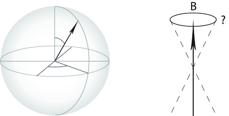
Figure 1: Spin in fluctuating magnetic field. The space of pure states of a spin-$\frac{1}{2}$ particle, in external magnetic field ${\bf B}$, is the surface of the Bloch sphere. In statistical theory of quantum mechanics the state is represented by statistical distributions of the pure states, whereas the magnetic field ${\bf B}$ that specifies the Hamiltonian is held fixed. What happens if the direction of the field ${\bf B}$ is itself subject to a small fluctuation?

2 Approach to equilibrium

In classical statistical mechanics the notion of a gradient flow plays an important role in describing the approach to equilibrium: A system immersed in a heat bath naturally tends to release its energy into the environment and thus approach its minimum energy state, and this tendency is characterised by a Hamiltonian gradient flow. An equilibrium state is attained when this flow is on average counterbalanced by thermal noise due to a random interaction with the bath. Here the magnitude of the noise is determined by the temperature of the bath. Accordingly, the idea we are going to introduce here is a gradient flow equation on the space of Hamiltonians with the property that the eigenstates of an arbitrary initial Hamiltonian $H_{0}$ at time $t=0$ tend toward alignment with those of a reference Hamiltonian, denoted by $G$. Thus, $G$ plays the role of the ‘fixed’ Hamiltonian in conventional quantum statistical mechanics. The eigenstates of $H_{t}$ thus evolve toward those of $G$ under the flow. By introducing a suitable noise term, we are able to characterise the approach to an equilibrium distribution.

The dynamical model for characterising approach to equilibrium is given by

$$\frac{{\rm d}H_{t}}{{\rm d}t}=-\lambda\left[H_{t},[H_{t},G]\right]+[H_{t},\omega_{t}],$$ (1)

where $\lambda\in{\mathds{R}}_{+}$. Here $\{\omega_{t}\}$ denotes a skew-symmetric matrix of independent white noise terms, and $[H_{t},\omega_{t}]$ is the Lie bracket of these with $H_{t}$ (see also [1]). Hence $[H_{t},\omega_{t}]$ is symmetric and linear in both $H_{t}$ and $\omega_{t}$. The term $\left[H_{t},[H_{t},G]\right]$ gives rise to the aforementioned gradient flow in the space of Hamiltonians. The Hermitian matrix $G$ plays the role of the ‘Hamiltonian of the Hamiltonians’ in the sense that $G$ determines the motion in the space of Hamiltonians. In particular, we can regard the linear function $\tr(HG)$ on the space of the totality of Hermitian matrices $H$ as representing the ‘energy’ function defined on that space.

There is an invariant measure (stationary solution) associated with the evolutionary equation (1). This is given by the canonical density:

$$\rho(H)\propto\exp\big{(}-\lambda\,{\rm tr}(HG)\big{)},$$ (2)

which can be used as a new basis for studying quantum statistical mechanics. In units $\hbar=1$ the coupling $\lambda$ has dimension $[{\rm Energy}]^{-1}$, and has the interpretation of representing the inverse temperature for the ‘Hamiltonian bath’ (not to be confused with the thermal bath in which the system, and possibly also the apparatus determining the Hamiltonian, is immersed). The canonical density (2) can also be derived by entropy maximisation subject to the constraint that the energy $\tr(HG)$ has a definite expectation value.

3 The gradient flow: double bracket equation

Let us begin by examining properties of the gradient term in (1). Specifically, consider the following dynamical equation for Hermitian matrices:

$$\frac{{\rm d}H_{t}}{{\rm d}t}=-\lambda\left[H_{t},[H_{t},G]\right].$$ (3)

Note that in terms of the Hermitian matrix $X={\rm i}[H,G]$ the double-bracket evolution (3) can be rewritten as

$$\frac{{\rm d}H}{{\rm d}t}={\rm i}\lambda[H,X],$$ (4)

which formally is just the Heisenberg equation of motion. However, owing to the $H$-dependence of $X$ the evolution is nonunitary. The Hamiltonians $H_{0}$ and $G$ are both assumed nondegenerate. The flow induced by (3) satisfies the following properties: (i) the evolution is isospectral, i.e. the eigenvalues of $H_{0}$ are preserved; and (ii) the evolution gives the ‘alignment’ $\lim_{t\to\infty}[H_{t},G]=0$.

We remark that the double bracket flow was first introduced in the context of magnetism (Landau-Lifshitz equation) [2]. In its modern form it was introduced by Brockett [3] and has been successfully applied to many areas, such as optimal control, linear programming, sorting algorithms, and dissipative systems (see references cited in [4]).

In the case of a $2\times 2$ Hamiltonian the gradient flow equation (3) can be solved straightforwardly. In this case we express the Hamiltonian in terms of the Pauli matrices:

$$H_{t}=\mbox{$\textstyle\frac{1}{2}$}\,u_{t}{\mathds{1}}+\mbox{$\textstyle\frac{1}{2}$}\,\nu\,{\boldsymbol{\sigma}}\!\cdot\!{\mathbf{n}}_{t},$$ (5)

where ${\mathbf{n}}_{t}=({\rm x}_{t},{\rm y}_{t},{\rm z}_{t})$. Similarly for the reference Hamiltonian $G$ we write

$$G=\mbox{$\textstyle\frac{1}{2}$}\,v{\mathds{1}}+\mbox{$\textstyle\frac{1}{2}$}\,\mu\,{\boldsymbol{\sigma}}\!\cdot\!{\mathbf{g}}$$ (6)

for a unit vector ${\mathbf{g}}$. A calculation shows that the solution to (3) reads

$$H_{t}=\mbox{$\textstyle\frac{1}{2}$}\!\left(\!\begin{array}[]{cc}u_{0}\!-\!\nu\tanh(\omega t-c_{0})&\nu\,{\rm sech}(\omega t-c_{0})\,{\rm e}^{-{\rm i}\phi_{0}}\\ \nu\,{\rm sech}(\omega t-c_{0})\,{\rm e}^{{\rm i}\phi_{0}}&u_{0}\!+\!\nu\tanh(\omega t-c_{0})\end{array}\!\right)\!,$$ (9)

where $\omega=\lambda\nu\mu$, and $c_{0}=\tanh^{-1}(\cos\theta_{0})$ and $\phi_{0}$ are initial values [4]. Furthermore, the eigenvalues of $H_{t}$ are time-independent, and we have

$$\lim_{t\to\infty}H_{t}=\mbox{$\textstyle\frac{1}{2}$}\left(\begin{array}[]{cc}u_{0}-\nu&0\\ 0&u_{0}+\nu\end{array}\right).$$ (12)

Thus, the Hamiltonian is asymptotically diagonalised in the $G$-basis. Observe that ${\rm tr}H_{t}$ and ${\det}H_{t}$ are conserved quantities. Therefore, the flow induced by (3) for fixed initial values $u_{0}$ and $|{\bf n}_{0}|$ is confined to a two-sphere ${\mathcal{L}}$, which is isomorphic to the state space of a two-level system. It follows that in two dimensions we have the equivalence of the Schrödinger and Heisenberg pictures, even though the dynamical equation is not unitary. Since $u_{0}$ and $|{\bf n}_{0}|$ are constant, we fix these and focus our attention on ${\mathcal{L}}$ parameterised by the dynamical coordinates $(\theta_{t},\phi_{t})$.

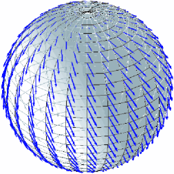
Figure 2: Gradient flow with unitary motion on the sphere ${\mathcal{L}}$. The vector field generated by the unitarily-modified gradient-flow (13) is plotted. The first term in (13) generates a rotation around the $G$-axis (which is chosen to be the $z$ axis here), while the second term generates geodesic flows toward the south pole. The axis ${\mathbf{n}}_{0}$ of the initial Hamiltonian $H_{0}$ spirals around the $G$-axis ${\mathbf{g}}$ and is asymptotically aligned with the latter (south pole in this example).

We remark that the dynamical equation (3) can be modified to include a unitary term:

$$\frac{{\rm d}H_{t}}{{\rm d}t}=-{\rm i}[H_{t},G]-\lambda\left[H_{t},[H_{t},G]\right]$$ (13)

without greatly affecting its physical characteristics. In the $2\times 2$ example, the only change occurs in the phase so that instead of $\phi_{t}=\phi_{0}$ we have $\phi_{t}=\phi_{0}+\mu t$.

4 Elements of stochastic differential geometry

We now wish to introduce a Brownian term into the deterministic flow (3). Specifically, we consider a uniform Brownian field on the isospectral subspace of the space of Hermitian matrices (the sphere ${\mathcal{L}}$ in the $2\times 2$ case). Before we proceed, however, it will be useful to recall how stochastic motions can be defined on a manifold. The basic process we consider is the Wiener process $\{W_{t}\}$ defined on a filtered probability space $({\Omega},{\cal F},{\mathbb{P}})$. Here ${\Omega}$ is the sample space, ${\cal F}$ is a $\sigma$-field on ${\Omega}$, and ${\mathbb{P}}$ is the probability measure. The filtration of ${\mathcal{F}}$ determines the causal structure of $({\Omega},{\cal F},{\mathbb{P}})$. This is given by a parameterised family $\{{\mathcal{F}}_{t}\}_{0\leq t<\infty}$ of nested $\sigma$-subfields satisfying ${\mathcal{F}}_{s}\subset{\mathcal{F}}_{t}\subset{\mathcal{F}}$ for any $s\leq t<\infty$. We say that $\{W_{t}\}$ is a Wiener process if: (a) $W_{0}=0$; and (b) $\{W_{t}\}$ is Gaussian such that $W_{t+h}-W_{t}$ has mean zero and variance $|h|$ (see [5]). A process $\{\sigma_{t}\}$ is said to be adapted to the filtration $\{{\cal F}_{t}\}$ generated by $\{W_{t}\}$ if its random value at time $t$ is determined by the history of $\{W_{t}\}$ up to that time.

If $\{\sigma_{t}\}$ is ${\cal F}_{t}$-adapted, then the stochastic integral $M_{t}=\int_{0}^{t}\sigma_{s}{\rm d}W_{s}$ exists, provided that $\{\sigma_{t}\}$ is almost surely square-integrable. If the variance of $\{M_{t}\}$ exists, then $\{M_{t}\}$ satisfies the martingale conditions ${\mathbb{E}}[|M_{t}|]<\infty$ and ${\mathbb{E}}[M_{t}|{\cal F}_{s}]=M_{s}$, where ${\mathbb{E}}[-]$ denotes expectation with respect to the measure ${\mathbb{P}}$. The latter condition implies that given the history of the Wiener process up to time $s$ the expectation of $M_{t}$ for $t\geq s$ is given by its value at $s$.

A general Ito process is defined by an integral of the form

$$x_{t}=x_{0}+\int_{0}^{t}\mu_{s}{\rm d}s+\int_{0}^{t}\sigma_{s}{\rm d}W_{s},$$ (14)

where $\{\mu_{t}\}$ and $\{\sigma_{t}\}$ are called the drift and the volatility of $\{x_{t}\}$. A convenient way of expressing (14) is to write ${\rm d}x_{t}=\mu_{t}{\rm d}t+\sigma_{t}{\rm d}W_{t}$, and to regard the initial condition $x_{0}$ as implicit. In the special case $\mu_{t}=\mu(x_{t})$ and $\sigma_{t}=\sigma(x_{t})$, where $\mu(x)$ and $\sigma(x)$ are prescribed functions, the process $x_{t}$ is said to be a diffusion.

This analysis can be generalised to the case of a diffusion $\{x_{t}\}$ taking values on a manifold ${\mathfrak{M}}$, driven by an $m$-dimensional Wiener process $\{W_{t}^{i}\}_{i=1,\ldots,m}$. Let $\nabla_{a}$ be a torsion-free connection on ${\mathfrak{M}}$ such that for any vector field $\xi^{a}$ its covariant derivative in local coordinates is

$$\delta_{\bf b}^{b}\delta_{a}^{\bf a}(\nabla_{b}\xi^{a})=\frac{\partial\xi^{\bf a}}{\partial x^{\bf b}}+\Gamma_{\bf bc}^{\bf a}\xi^{\bf c},$$ (15)

where $\delta_{a}^{\bf a}$ is the standard coordinate basis in a given coordinate patch. Suppose we have an Ito process taking values in ${\mathfrak{M}}$. Let $x_{t}^{\bf a}$ denote the coordinates of the process in a particular patch. Then writing $h^{\bf ab}=\sigma_{i}^{\bf a}\sigma^{{\bf b}i}$ we define the drift process $\mu^{\bf a}$ by

$$\mu^{\bf a}{\rm d}t={\rm d}x^{\bf a}+\mbox{$\textstyle\frac{1}{2}$}\Gamma_{\bf bc}^{\bf a}h^{\bf bc}{\rm d}t-\sigma_{i}^{\bf a}{\rm d}W_{t}^{i}.$$ (16)

Alternatively, we can write the covariant Ito differential as ${\rm d}x^{a}=\delta_{\bf a}^{a}({\rm d}x^{\bf a}+\mbox{$\textstyle\frac{1}{2}$}\Gamma_{\bf bc}^{\bf a}h^{\bf bc}{\rm d}t)$, where $\delta^{a}_{\bf a}$ is the dual coordinate basis. Then (16) can be represented as

$${\rm d}x^{a}=\mu^{a}{\rm d}t+\sigma^{a}_{i}{\rm d}W^{i}_{t}.$$ (17)

If $\mu^{a}(x)$ and $\sigma^{a}_{i}(x)$ are $m+1$ vector fields on ${\mathfrak{M}}$, then the general diffusion process on ${\mathfrak{M}}$ is governed by a stochastic differential equation ${\rm d}x^{a}=\mu^{a}(x){\rm d}t+\sigma^{a}_{i}(x){\rm d}W^{i}_{t}$, where ${\rm d}x^{a}$ is the covariant Ito differential associated with the given connection (see Hughston [6]).

For the characterisation of the diffusion process it suffices to specify a connection on ${\mathfrak{M}}$, and a metric is not required. The quadratic relation ${\rm d}x^{a}{\rm d}x^{b}=h^{ab}{\rm d}t$, where $h^{ab}=\sigma_{i}^{a}\sigma^{bi}$, follows from the Ito identities ${\rm d}t^{2}=0$, ${\rm d}t{\rm d}W_{t}^{i}=0$, and ${\rm d}W_{t}^{i}{\rm d}W_{t}^{j}=\delta^{ij}{\rm d}t$. Then for any smooth function $\phi(x)$ on ${\mathfrak{M}}$ we define the associated process $\phi_{t}=\phi(x_{t})$, and Ito’s formula takes the form

$${\rm d}\phi_{t} = (\nabla_{a}\phi){\rm d}x^{a}+\mbox{$\textstyle\frac{1}{2}$}(\nabla_{a}\nabla_{b}\phi){\rm d}x^{a}{\rm d}x^{b}$$ (18)

$$= \left(\mu^{a}\nabla_{a}\phi+\mbox{$\textstyle\frac{1}{2}$}h^{ab}\nabla_{a}\nabla_{b}\phi\right){\rm d}t+\sigma^{a}_{i}\nabla_{a}\phi{\rm d}W^{i}_{t}.$$

The probability law for $x_{t}$ is characterised by a density function $\rho(x,t)$ on ${\mathfrak{M}}$ that satisfies the Fokker-Planck equation

$$\frac{\partial\rho}{\partial t}=-\nabla_{a}(\mu^{a}\rho)+\mbox{$\textstyle\frac{1}{2}$}\nabla_{a}\nabla_{b}(h^{ab}\rho).$$ (19)

The diffusion is said to be nondegenerate if $h^{ab}$ is of maximal rank. If $g_{ab}$ is a Riemannian metric on ${\mathfrak{M}}$ and $\nabla_{a}$ is the associated Levi-Civita connection, then if $h^{ab}=\sigma^{2}g^{ab}$, the process $x_{t}$ is a Brownian motion with drift on ${\mathfrak{M}}$, with volatility parameter $\sigma$.

5 Diffusion model for thermalisation

Consider a stochastic differential equation of the form

$${\rm d}x^{a}=\mu^{a}{\rm d}t+\kappa\sigma^{a}_{i}{\rm d}W_{t}^{i}$$ (20)

on a real manifold ${\mathfrak{M}}$. Here $\kappa$ is a constant, the drift $\mu^{a}$ is a vector field on ${\mathfrak{M}}$, and the vectors $\{\sigma^{a}_{i}\}$ constitute an orthonormal basis in the tangent space of ${\mathfrak{M}}$. In this case the associated Fokker-Planck equation reads

$$\frac{\partial}{\partial t}\,\rho_{t}(x)=-\nabla_{a}(\mu^{a}\rho_{t})+\mbox{$\textstyle\frac{1}{2}$}\kappa^{2}\nabla^{2}\rho_{t}.$$ (21)

For our model we require that the drift vector $\mu^{a}$ represent the double-bracket gradient flow (3). This is achieved by choosing

$$\mu^{a}=-\mbox{$\textstyle\frac{1}{2}$}\,\kappa^{2}\lambda\nabla^{a}G,$$ (22)

where $G(x)$ is a function on ${\mathfrak{M}}$ given by $\tr(HG)$. Then it follows that there exists a unique stationary solution to (21), given by the canonical density

$$\rho(x)=\frac{\exp(-\lambda G(x))}{\int_{\mathfrak{M}}\exp(-\lambda G(x)){\rm d}V}.$$ (23)

If ${\mathfrak{M}}$ is the space of pure states, then we have a model for thermalisation of quantum states introduced by Brody & Hughston [7].

6 Two-dimensional case in more detail

To illustrate these results in more explicit terms we consider a system consisting of a single spin-$\frac{1}{2}$ particle immersed in an external magnetic field. The Hamiltonian is then $H=-{\mathbf{B}}\cdot{\mathbf{S}}$, where ${\mathbf{B}}$ denotes the field and ${\mathbf{S}}$ the spin vector. The direction of the field ${\mathbf{B}}$, however, is subject to fluctuations around its stable direction, specified by $G$ (directed along the $z$-axis). For the dynamical equation we obtain [4]:

$$\left\{\begin{array}[]{l}\rm d\theta_{t}=\omega\,\sin\theta_{t}{\rm d}t+\sqrt{2\nu}({\rm d}W_{t}^{1}+{\rm d}W_{t}^{2})\\ {\rm d}\phi_{t}=-\frac{1}{\sin\theta_{t}}\sqrt{2\nu}({\rm d}W_{t}^{1}-{\rm d}W_{t}^{2}).\end{array}\right.$$ (26)

The associated Fokker-Planck equation reads

$${\dot{\rho}}=-\omega(\cos\theta+\sin\theta\,\partial_{\theta})\rho+2\nu{\textstyle{\left(\partial_{\theta}^{2}\!+\frac{1}{\sin^{2}\theta}\,\partial_{\phi}^{2}\right)}}\rho,$$ (27)

where $\partial_{\theta}=\partial/\partial\theta$ and $\partial_{\phi}=\partial/\partial\phi$. The asymptotic solution is the canonical density function:

$$\rho(\theta,\phi)=\frac{\lambda\mu}{2\pi\sinh(\frac{1}{2}\lambda\mu)}\,\exp\left(-\mbox{$\textstyle\frac{1}{2}$}\lambda\mu\cos\theta\right).$$ (28)

Direct substitution shows that (28) is the stationary solution to (27).

It follows from (28) and the use of the volume element ${\rm d}V=\frac{1}{4}\sin\theta{\rm d}\theta{\rm d}\phi$ that the equilibrium mean Hamiltonian is

$$\langle H\rangle=\mbox{$\textstyle\frac{1}{2}$}\left(\begin{array}[]{cc}u_{0}+\nu\langle\cos\theta\rangle_{\lambda}&0\\ 0&u_{0}-\nu\langle\cos\theta\rangle_{\lambda},\end{array}\right),$$ (31)

where

$$\langle\cos\theta\rangle_{\lambda}=\frac{2}{\lambda\mu}-\frac{1}{\tanh(\frac{1}{2}\lambda\mu)}.$$ (32)

We may regard the parameter $\lambda$ as representing the ‘inverse temperature’ for the Hamiltonian. If the noise level is high ($\lambda\ll 1$), then the direction of the external field ${\mathbf{B}}$ on the average lies close to the $xy$-plane so that $\langle\cos\theta\rangle_{\lambda}\simeq 0$. If the noise level is low $\lambda\gg 1$, then the field ${\mathbf{B}}$ on the average is parallel to the $z$-axis and we have $\langle\cos\theta\rangle_{\lambda}\simeq-1$. We plot $\langle\cos\theta\rangle_{\lambda}$ as a function of $\tau=1/\lambda$ (see Fig. 3).

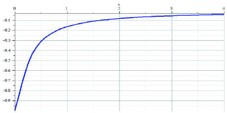
Figure 3: The plot of the expectation $\langle\cos\theta\rangle_{\lambda}$ as a function of the inverse Hamiltonian temperature $\tau=1/\lambda$. For $\tau\ll 1$ we have $\langle\cos\theta\rangle_{\lambda}\simeq-1$, whereas for $\tau\gg 1$ we find $\langle\cos\theta\rangle_{\lambda}\simeq 0$.

7 Quantum statistical mechanics of disordered systems

Now we consider how the statistical theory of Hamiltonians presented above can be applied to quantum statistical mechanics, when the system and the apparatus specifying the Hamiltonian are both immersed in a heat bath with inverse temperature $\beta$. In this context it is natural to borrow ideas from the spin glass literature. We may take the averaged Hamiltonian $\langle H\rangle_{\lambda}$ as the starting point of the analysis—this gives the analogue of an annealed average:

$$\langle O\rangle_{A}=\frac{{\rm tr}\left(O{\rm e}^{-\beta\langle H\rangle_{\lambda}}\right)}{{\rm tr}\left({\rm e}^{-\beta\langle H\rangle_{\lambda}}\right)}$$ (33)

of an observable $O$. Such an averaging, however, will change the eigenvalues of $H$.

Alternatively, we may use the ‘unaveraged’ Hamiltonian to compute the expectation of an observable $O$, and then take its average:

$$\langle O\rangle_{Q}=\left\langle\frac{{\rm tr}(O{\rm e}^{-\beta H})}{{\rm tr}({\rm e}^{-\beta H})}\right\rangle_{\lambda}.$$ (34)

This gives the analogue of a quenched average. The canonical quenched average of the Hamiltonian $G=\sigma_{z}$ is

$$\langle G\rangle_{Q}=\mbox{$\textstyle\frac{1}{2}$}\mu\,{\textstyle\tanh\left(\mbox{$\textstyle\frac{1}{2}$}\beta\nu\right)\left(\frac{1}{\tanh\left(\frac{1}{2}\lambda\mu\right)}-\frac{2}{\lambda\mu}\right)},$$ (35)

whereas the canonical annealed average of $G$ is

$$\langle G\rangle_{A}=\mbox{$\textstyle\frac{1}{2}$}\mu\,{\textstyle\tanh\left[\mbox{$\textstyle\frac{1}{2}$}\beta\nu\left(\frac{1}{\tanh\left(\frac{1}{2}\lambda\mu\right)}-\frac{2}{\lambda\mu}\right)\right]}.$$ (36)

These results suggest a new line of studies on the extended quantum statistical mechanics of disordered systems. The plot below shows the annealed (blue) and quenched (red) averages of $\sigma_{z}$, as a function of the bath temperature $T=1/\beta$, for fixed $\lambda$ such that $\lambda^{-1}=0.1$.

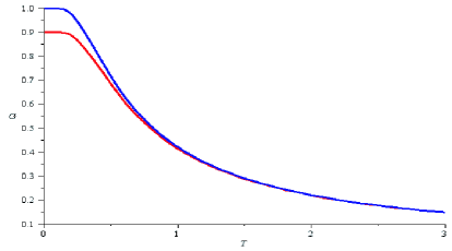
Figure 4: Quenched and annealed averages of $G$. The functions $\langle G\rangle_{Q}$ and $\langle G\rangle_{A}$ are plotted against the temperature $T=\beta^{-1}$, where we set $\lambda^{-1}=0.1$, $v=0$, $\nu=1$, and $\mu=2$ so that $G=\sigma_{z}$. The ‘quenched magnetisation’ $\langle\sigma_{z}\rangle_{Q}$ does not attain the maximum value $1.0$ at zero temperature unless $\lambda^{-1}=0$.

8 Examination of higher-dimensional cases

The geometry of higher-dimensional Hermitian matrices is somewhat more intricate than the two-dimensional case examined above. The space of $N\times N$ Hermitian matrices has the structure of the product ${\mathds{R}}^{N}\times\mathbb{CP}^{N}\times\mathbb{CP}^{N-1}\times\cdots\times\mathbb{CP}^{1}$, where $\mathbb{CP}^{k}$ denotes the complex projective $k$-space. This space is considerably larger than the space $\mathbb{CP}^{N}$ of pure states upon which $N\times N$ Hermitian matrices act, and as a consequence the equivalence of the Schrödinger and Heisenberg pictures for a nonunitary motion would in general be lost.

A $3\times 3$ Hermitian matrix $H$ can be written as $H=E_{1}|E_{1}\rangle\langle E_{1}|+E_{2}|E_{2}\rangle\langle E_{2}|+E_{3}|E_{3}\rangle\langle E_{3}|$, where $\{E_{i}\}$ are the eigenvalues and $\{|E_{i}\rangle\}$ are the associated eigenstates. The degrees of freedom for the energy eigenvalues correspond to the open space ${\mathds{R}}^{3}$; the remaining degrees of freedom corresponding to $\mathbb{CP}^{2}\times\mathbb{CP}^{1}$ are encoded in the specification of the energy eigenstates. Writing $\{|g_{i}\rangle\}$ for the eigenstates of $G$, we can express $|E_{1}\rangle$ in the form:

$$|E_{1}\rangle=\sin\mbox{$\textstyle\frac{1}{2}$}\vartheta\cos\mbox{$\textstyle\frac{1}{2}$}\varphi|g_{1}\rangle+\sin\mbox{$\textstyle\frac{1}{2}$}\vartheta\sin\mbox{$\textstyle\frac{1}{2}$}\varphi{\rm e}^{{\rm i}\xi}|g_{2}\rangle+\cos\mbox{$\textstyle\frac{1}{2}$}\vartheta{\rm e}^{{\rm i}\eta}|g_{3}\rangle,$$ (37)

which determines a point in $\mathbb{CP}^{2}$. There is a $\mathbb{CP}^{1}$ worth degrees of freedom left for $|E_{2}\rangle$:

$$|E_{2}\rangle = \left(\cos\mbox{$\textstyle\frac{1}{2}$}\alpha\sin\mbox{$\textstyle\frac{1}{2}$}\vartheta\cos\mbox{$\textstyle\frac{1}{2}$}\varphi-\sin\mbox{$\textstyle\frac{1}{2}$}\alpha\sin\mbox{$\textstyle\frac{1}{2}$}\varphi{\rm e}^{{\rm i}\beta}\right)|g_{1}\rangle$$ (38)

$$+\left(\cos\mbox{$\textstyle\frac{1}{2}$}\alpha\cos\mbox{$\textstyle\frac{1}{2}$}\vartheta\sin\mbox{$\textstyle\frac{1}{2}$}\varphi{\rm e}^{{\rm i}\xi}+\sin\mbox{$\textstyle\frac{1}{2}$}\alpha\cos\mbox{$\textstyle\frac{1}{2}$}\varphi{\rm e}^{{\rm i}(\beta+\xi)}\right)|g_{2}\rangle+\cos\mbox{$\textstyle\frac{1}{2}$}\alpha\sin\mbox{$\textstyle\frac{1}{2}$}\vartheta{\rm e}^{{\rm i}\eta}|g_{3}\rangle.$$

The specifications of $|E_{1}\rangle$ and $|E_{2}\rangle$ leave no further freedom left for $|E_{3}\rangle$ and we have

$$|E_{3}\rangle = \left(\sin\mbox{$\textstyle\frac{1}{2}$}\alpha\cos\mbox{$\textstyle\frac{1}{2}$}\vartheta\cos\mbox{$\textstyle\frac{1}{2}$}\varphi+\cos\mbox{$\textstyle\frac{1}{2}$}\alpha\sin\mbox{$\textstyle\frac{1}{2}$}\varphi{\rm e}^{{\rm i}\beta}\right)|g_{1}\rangle$$ (39)

$$+\left(\sin\mbox{$\textstyle\frac{1}{2}$}\alpha\cos\mbox{$\textstyle\frac{1}{2}$}\vartheta\sin\mbox{$\textstyle\frac{1}{2}$}\varphi{\rm e}^{{\rm i}\xi}-\cos\mbox{$\textstyle\frac{1}{2}$}\alpha\cos\mbox{$\textstyle\frac{1}{2}$}\varphi{\rm e}^{{\rm i}(\beta+\xi)}\right)|g_{2}\rangle+\sin\mbox{$\textstyle\frac{1}{2}$}\alpha\sin\mbox{$\textstyle\frac{1}{2}$}\vartheta{\rm e}^{{\rm i}\eta}|g_{3}\rangle.$$

In this manner we obtain the nine parameters required for the specification of an arbitrary $3\times 3$ Hermitian matrix.

It should be remarked that the foregoing procedure is merely an example of how one might parameterise a generic $N\times N$ Hermitian matrix in a systematic manner; the scheme is somewhat unconventional in that a generic $2\times 2$ Hermitian matrix in this parameterisation is written

$$H=\omega_{+}\left(\begin{array}[]{cc}1&0\\ 0&1\end{array}\right)+\omega_{-}\left(\begin{array}[]{cc}\cos\theta&\sin\theta\,{\rm e}^{-{\rm i}\phi}\\ \sin\theta\,{\rm e}^{{\rm i}\phi}&-\cos\theta\end{array}\right),$$ (44)

where $\omega_{\pm}=\frac{1}{2}(E_{1}\pm E_{2})$. This set of coordinates is nevertheless convenient because it isolates invariant quantities $\omega_{\pm}$ from the coordinates $(\theta,\phi)$ of the isospectral submanifolds.

For our application in quantum statistical mechanics of disordered systems we are required to determine the partition function

$$Z(\lambda)=\int{\rm e}^{-\lambda\tr(HG)}{\rm d}V.$$ (45)

In the case of a $3\times 3$ Hamiltonian, since the dynamical equation (1) preserves the three eigenvalues of $H$, the dynamical motion stays on the isospectral submanifold spanned by the six angular variables $\vartheta,\varphi,\alpha\in[0,\pi]$ and $\xi,\eta,\beta\in[0,2\pi]$, with volume element

$${\rm d}V={\textstyle\frac{1}{128}}\sin\alpha\sin\vartheta(1-\cos\vartheta)\sin\varphi\,{\rm d}\alpha\,{\rm d}\beta\,{\rm d}\vartheta\,{\rm d}\varphi\,{\rm d}\xi\,{\rm d}\eta.$$ (46)

Since we are working in the $G$-basis, the calculation of $\tr(HG)$ is straightforward, and the integral (45) reduces to an expression analogous to the integral representation for a Bessel function.

The choice of parameterisation adapted here for a generic $N\times N$ Hermitian matrix need not be the most adequate for our purpose. An alternative approach is to write $H=U^{\dagger}EU$, where $E$ is a diagonal matrix with eigenvalues $\{E_{i}\}$, and $U$ is a unitary matrix. Then the calculation of the partition function becomes semi-Gaussian, and we are left with an integration over the invariant Haar measure [8]. Ideas from matrix theory or random matrices might prove useful in the statistical analysis of disordered quantum systems introduced here.

The authors thank R. Brockett and E. J. Brody for comments and stimulating discussions. DDH thanks the Royal Society of London for partial support by its Wolfson Merit Award.

References

[1] Brockett, R. W. “Notes on stochastic
processes on manifolds” In Systems and Control in the
Twenty-First Century (C. Byrnes, et al., eds.) pp. 75-101,
(Boston: Birkhäuser, 1997).
[2] Landau, L. D. and Lifshitz, E. M.
“On the theory of the dispersion of magnetic permeability in
ferromagnetic bodies” Phys. Z. Sowietunion8 153-169
(1935).
[3] Brockett, R. W. “Dynamical systems that sort
lists, diagonalise matrices, and solve linear programming problems”
Lin. Alg. Appl.146 79-91 (1991).
[4] Brody, D. C., Ellis, D.C.P., and Holm, D.D.
“Hamiltonian statistical mechanics” J. Phys. A41
502002 (2008).
[5] Hida, T. Brownian Motion. (Berlin, Germany:
Springer, 1980).
[6] Hughston, L. P. “Geometry of stochastic state
vector reduction” Proc. Roy. Soc. London A452
953-979 (1996).
[7] Brody, D. C. and Hughston, L. P. “Thermalisation
of quantum states” J. Math. Phys.40 12-18 (1999).
[8] Sugiura, M. Unitary Representations and
Hamonic Analysis (Amsterdam: North-Holland, 1990).