Critical current of a Josephson junction containing a conical magnet

Abstract

We calculate the critical current of a superconductor/ferromagnetic/superconductor (S/FM/S) Josephson junction in which the FM layer has a conical magnetic structure composed of an in-plane rotating antiferromagnetic phase and an out-of-plane ferromagnetic component. In view of the realistic electronic properties and magnetic structures that can be formed when conical magnets such as Ho are grown with a polycrystalline structure in thin-film form by methods such as direct current sputtering and evaporation, we have modeled this situation in the dirty limit with a large magnetic coherence length ($\xi_{f}$). This means that the electron mean free path is much smaller than the normalized spiral length $\lambda/2\pi$ which in turn is much smaller than $\xi_{f}$ (with $\lambda$ as the length a complete spiral makes along the growth direction of the FM). In this physically reasonable limit we have employed the linearized Usadel equations: we find that the triplet correlations are short ranged and manifested in the critical current as a rapid oscillation on the scale of $\lambda/2\pi$. These rapid oscillations in the critical current are superimposed on a slower oscillation which is related to the singlet correlations. Both oscillations decay on the scale of $\xi_{f}$. We derive an analytical solution and also describe a computational method for obtaining the critical current as a function of the conical magnetic layer thickness.

I Introduction

The interaction of singlet-type superconductors (S) with ferromagnetic materials in S/FM hybrid systems is a field of extensive and ongoing research (see Refs. ReviewBuzd2005 ; Bergeret2001 ; ReviewBerg2005 and references therein). In proximity, the interaction of these competing electron orders is characterized by an oscillating component in the Cooper pair wave function which leads to a number of interesting phenomena: the critical superconducting temperature $T_{c}$ dependence of S/FM bilayers on FM layer thickness $d_{f}$,Tc oscillations in SF bilayers1 ; Tc oscillations in SF bilayers2 ; Tc oscillations in SF bilayers3 ; Tc oscillations in SF bilayers4 dependence of $T_{c}$ on the orientation of FM layers in FM^′/S/FM^′′ spin valves F/S/F type memory devices1 ; F/S/F type memory devices2 ; F/S/F type memory devices3 ; F/S/F type memory devices4 ; F/S/F type memory devices5 ; F/S/F type memory devices6 and S/FM^′/FM^′′ multilayers, and finally the realization of $\pi$ coupling in S/FM/S Josephson junctions. ZeroPi1 ; ZeroPi2 ; ZeroPi3 ; ZeroPi4 ; ZeroPi5

The standard analysis of the S/FM systems has mostly assumed that the FM is homogeneous and collinear, in which case only the singlet superconducting correlation appears in the theory. Extending this standard approach, theory strongly indicates that if the FM is inhomogeneous and noncollinear, the longer-ranged triplet superconducting correlations should then emerge at the S/FM interface.ReviewBuzd2005 ; Bergeret2001 ; ReviewBerg2005 These triplet correlations should then be insensitive to the exchange field of the FM material and as such their proximity range is expected to be similar to that of singlet pairs in a superconductor/normal metal system.

Inhomogeneous magnetization exists in a range of material systems, which can be classified into three categories: (1) magnetic domain walls; (2) ferromagnetic multilayers such as when FM layers are decoupled via a nonmagnetic (NM) spacer to form spin-active devices; and (3) the intrinsically inhomogeneous and noncollinear magnetic materials.

Domain walls were one of the first magnetically inhomogeneous systems to be combined with superconductivity. Although experimental studies of such systems are notoriously challenging because of the need to control the magnetism at the nanometer scale, results and analysis have indicated that domain walls are favorable nucleation sites for superconductivity.DomainWallSC1 ; DomainWallSC2 ; DomainWallSC3 ; DomainWallSC4 ; DomainWallSC5 Theoretically, the emergence of triplet components in junctions containing a single domain wall and or a multidomain ferromagnet (MDFM) have been extensively analyzed.SingleDomainWallJunctions1 ; SingleDomainWallJunctions2 Recently, large area S/MDFM/S junctions have been fabricated.TruptiPdNi2009 In this type of junction, the amplitude of the critical current is expected to decay exponentially with FM layer thickness. If singlet-type electron pairs are scattered into triplet ones at the domain-wall regions, it is expected that for a critical thickness of the MDFM the triplet correlations will dominate over the singlet ones leading to slower decay in the critical current with the MDFM thickness. So far, evidence of a crossover from singlet to triplet-dominated transport in these types of systems is nonexistent.

The second category, the ferromagnetic multilayers, have been combined with superconductors in S/FM^′/FM^′/S junction form junction form although most studies have been theoretical up to nowSFISF1 ; SFISF2 ; SFISF3 ; SFISF4 with only a few experiments showing how the Josephson ground state is affected by the orientation of the FM layers.SFISF5 ; SFISF6 The majority of experimental studies have focused on how a superconducting layer is modified by the relative orientation of the FMs. In these systems, however, the triplet superconducting components that exist when the FMs are noncollinear only transmit information about the direction of the magnetic layers.Zimansky ; Parity To observe a longer-ranged spin triplet proximity effect, it is thought that the Josephson junction must contain three more FMs,SFISF4 ; Houzet2007 with each offset from the other by an angle $\theta\neq[0,\pi]$ (with $\pi$ as the antiparallel configuration). In principle, the angle $\theta$ and thus the triplet components could be controlled by the application of an external magnetic field. Unfortunately, the implementation of a large enough change in the angle $\theta$ with an applied magnetic field is very difficult to realize without strongly suppressing the superconductivity.

The third category, the intrinsically noncollinear magnets, is potentially one of the simplest systems to combine with a superconductor to experimentally study triplet correlations.Linder2009 Recently,Sosnin2006 interferometer measurements of superconducting Al coupled to the rare-earth metal Ho have been made. In these Al/Ho/Al junctions, superconducting phase periodic conductance oscillations were observed indicating the presence of a longer-ranged proximity effect when interpreted in the limit of a small coherence length in the Ho relative to the length of a complete spiral $\lambda$.Volkov2006 It is understood that the triplet correlations were generated at the Al/Ho interface due to a rotating magnetization present there and sustained by a continuous magnetic spiral throughout the length of the Ho. A similar explanationHalfMetal2 ; HalfMetal3 ; HalfMetal4 ; HalfMetal5 was given for a long-ranged proximity effect observed in the half-metal CrO₂.HalfMetal1 In this system, the triplet current was shown to be insensitive to the strong polarization of the half metal. Spin mixing at the interface is currently the best explanation for the triplet proximity effect observed although a better understanding of the interfaces that can exist in these types of material systems is needed to verify this explanation. For Ho, it is well known that growing it in thin-film form with a magnetic spiral at the interface is difficult to achieve. This again highlights a need to improve our understanding of the likely properties and structures that can arise at the interface of noncollinear magnets, such as Ho, with superconducting materials.

The magnetic structureHo1 ; Ho2 ; Ho3 and electronic/thermal propertiesHo2 of the rare-earth Ho are well known. Its magnetic structure has been characterized in bulk, single crystal, and thin-film forms by neutron diffraction, x-ray diffraction, and vibrating sample magnetometery. In thin-film form, the quality of the conical magnetic structure is poorly understood although it is well known that the growth method and growth conditions, crystal forms, and interfacing materials affect the ordering range of the magnetic structure.Ho1 ; Ho2

Long-ranged magnetic ordering in Ho requires a coherent crystal structure in which the $c$ axis is the screw axis with the moments in the basal plane configured into a distorted helix parallel to the $c$ axis. The quality of the Ho (e.g., impurity content and roughness) and the strain at the NM/Ho interface are both important factors in determining the scale of magnetic ordering; for example, substantial intermixing at the NM/FM interface may disturb the growth in the helix which may affect, smear out, or even destroy any triplet correlations. Neutron-diffraction studies on epitaxial (interfacially strained) Nb/Ho bilayer films grown by dc magnetron sputteringHo4 at high temperature suggest the presence of an in-plane spiral (antiferromagnetic part) but no out-of-plane pitch (ferromagnetic part) was detected even down to very low temperatures $T\sim 1$ K. This implies that the strain at the Nb/Ho interface is suppressing the ferromagnetic component. Further studies on polycrystalline Nb/Ho/Nb trilayer films have also been made.Ho5 In these films strain at the Nb/Ho interface is lower and from Josephson-junction-type measurements a weakly conical magnetic structure was confirmed from field-dependent measurements of the junction’s critical current as a function of the Ho spacer layer thickness.

Altogether, the above review shows that although Ho can be grown on top of thick Nb leads with a conical magnetic structure, strain at the interface does weaken the ferromagnetic component possibly implying a weaker magnetism. The motivation behind this work is to complement the currently available theory on S/FM/S junctions with a conical FM weak link by considering the physically reasonable situation (see Sec. III) in which the conical ferromagnetic coherence length $\xi_{f}$ is much longer than the normalized spiral length $\lambda/2\pi$. Because both $\xi_{f}$ and $\lambda/2\pi$ are much larger than the electron mean free path $\ell$ (dirty limit), the S/FM/S junction can be described within the framework of the linearized Usadel equations.

This paper is organized as follows: Sec. II reviews the magnetic and electronic properties of thin-film Ho and outlines the important physical properties of the situation being analyzed in this paper; in Secs. III and IV, the general theoretical framework in which we model a Josephson junction containing a conical magnet is described with analytical solutions to obtain the Josephson current explained; in Sec. V, we present a computational method for calculating the Josephson current, which is particularly useful to experimentalists.

II Magnetic structure and electronic properties of thin-film Holmium

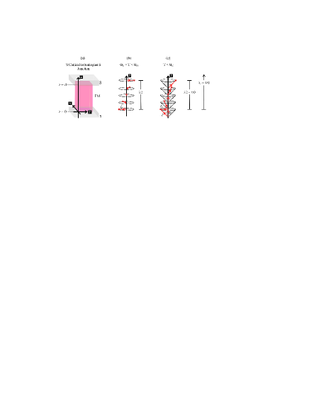
Figure 1: (Color online) (a) An illustration of two singlet-type superconductors (S) sandwiching a ferromagnet with a conical magnetic structure (Ho). The two magnetic phases of Ho, (b) the in-plane antiferromagnetic spiral phase of Ho below its Néel temperature $\Theta_{n}$, and (c) the conical magnet phase of Ho below its Curie temperature $\Theta_{c}$: the antiferromagnetic component $I_{r}$ rotating in the $\{x,y\}$ plane; the ferromagnetic component $I_{z}$ pitched towards the $z$ axis; and the resultant magnetization vector $\mathbf{I}$ rotating on the surface of a cone. In the limit considered in this paper, the ferromagnetic coherence length $\xi_{f}$ is much larger than $\lambda/2\pi$.

Consider the general structure of a conical magnet which consists of a rotating in-plane magnetization and a constant out-of-plane magnetization [see illustrations in Figs. 1(a)$-$1(c)]. The in-plane component is effectively an antiferromagnetic (AFM) state which orders itself at the Néel temperature $\Theta_{n}$, while the out-of-plane component can be considered to be a ferromagnetic phase which orders itself at the Curie temperature of the material. Thus, the strength or exchange interaction energy $I$ of the ferromagnetic part is related to the Curie temperature: $I\sim k_{B}\Theta_{c}$. The in-plane component completes a full rotation in a distance of $\lambda$ along the $z$ axis, which implies the distance along $z$ on which the in-plane component rotates in 1 rad is $\lambda/2\pi$. From now on, $\lambda/2\pi$ will be referred to as the normalized spiral length.

In the analysis that follows this section we shall assume that the electron mean-free path $\ell$ is smaller than both the coherence length of Ho $\xi_{f}$ and the normalized spiral length $\lambda/2\pi$. For Ho in thin-film form, this limiting situation is justified for the case when it is sputter deposited and polycrystalline.

Polycrystalline thin films of Ho have a large residual resistivity $\rho_{0}$ in the (6$-$12)$\times$10^-7 $\Omega$m range (see Refs. Ho3 and Ho5 and references therein). A rough estimate of the electron mean free path for the conduction electrons around 4 K using the relation $\ell=v_{F}m/\rho_{0}ne^{2}$, where $v_{F}$, the Fermi velocity is 1.6$\times$10⁶ m/s,Ho3 $m$ is the mass of the electron, and $n$ is the number density of free electrons, gives a (0.5$-$1.0) nm range, which is smaller than both $\xi_{f}\sim$ (6$-$7) nm and $\lambda/2\pi\sim$ 1.1 nm.Ho5 Even in single-crystal form, the resistivity of thin-film Ho is large and around 6$\times$10^-7 $\Omega$m with an electron mean-free path of $\sim$ 1.0 nm in the $c$-axis orientation.

III General solution in a conical ferromagnet

Let us consider a conical ferromagnet FM, the axis of which coincides with the $z$ axis. The magnetization vector and hence the exchange field $\mathbf{I}=(I_{x},I_{y},I_{z})$ has a constant axial component $I_{z}$ and a radial component $I_{r}$, which rotates in the $\{x,y\}$ plane with wave vector $Q=2\pi/\lambda$ as we move along the $z$ direction (see Fig. 1). The $x$ and $y$ components of $\mathbf{I}$ are therefore given by

$$I_{x}(z)=I_{r}\cos(Qz)\quad\textrm{and}\quad I_{y}(z)=I_{r}\sin(Qz).$$ (1)

In this section we find the solutions for the anomalous Green’s function in the conical FM, considering in particular the case of large $Q$. We assume that the dirty limit is fulfilled, which means that the FM coherence length ($\xi_{f}=\sqrt{\hbar D_{f}/|\mathbf{I}|}$ with $D_{f}$ being the diffusivity of the FM) and the normalized spiral length $\lambda/2\pi$ are both much larger than the electron mean free path, i.e. $\xi_{f},\lambda/2\pi\gg\ell$. If it is also assumed that the anomalous function is sufficiently small in the FM (which is the case if the S/FM interfacial resistance is large enough),ReviewBuzd2005 we can use the linearized Usadel equation Houzet2007

$$\hbar D_{f}\frac{d^{2}\hat{F}(z)}{dz^{2}}-2\hbar|\omega|\hat{F}(z)-\mathrm{sgn}(\omega)i[\mathbf{I}(z)\cdot\hat{\bm{\sigma}},\hat{F}(z)]_{+}=0,$$ (2)

where the anomalous Green’s function

$$\hat{F}=f_{0}\hat{1}+\mathbf{f}\cdot\hat{\bm{\sigma}}$$ (3)

is a matrix in spin space with $\mathbf{f}=(f_{x},f_{y},f_{z})$, and $\hat{\bm{\sigma}}=(\hat{\sigma}_{x},\hat{\sigma}_{y},\hat{\sigma}_{z})$ is a vector containing the Pauli matrices. The component $f_{0}$ is an even, while $f_{x}$, $f_{y}$ and $f_{z}$ are odd functions of the frequency $\omega$. The Matsubara frequencies are given by $\omega=(2n+1)\pi k_{B}T/\hbar$ with $n=0,\pm 1,\pm 2,...$ at temperature $T$ and $[a,b]_{+}=ab+ba$ is the anticommutator. If we substitute expression (3) into Eq. (2) we obtain a set of equations for the four components of the anomalous function $\hat{F}$,

$$\frac{1}{2}\hbar D_{f}\frac{d^{2}f_{0}(z)}{dz^{2}}-\hbar\omega f_{0}(z)-i[\mathbf{I}(z)\cdot\mathbf{f}(z)]=0,$$ (4)

$$\frac{1}{2}\hbar D_{f}\frac{d^{2}f_{x,y,z}(z)}{dz^{2}}-\hbar\omega f_{x,y,z}(z)-iI_{x,y,z}(z)f_{0}(z)=0.$$ (5)

Since the symmetric properties of the Usadel equations with respect to $\omega$ are trivial, only the case of $\omega>0$ is treated from now; we already omitted $\mathrm{sgn}(\omega)$ and used $\omega$ instead of $|\omega|$ in Eqs. (4) and (5). After putting expressions (1) into Eqs. (4) and (5), they can be simplified with the substitution $f_{\pm}=f_{x}\pm if_{y}$, which yields

$$\frac{d^{2}f_{0}}{dz^{2}}-2k_{\omega}^{2}f_{0}-i(2k_{z}^{2}f_{z}+k_{r}^{2}(f_{+}e^{-iQz}+f_{-}e^{iQz}))=0,$$ (6)

$$\frac{d^{2}f_{\pm}}{dz^{2}}-2k_{\omega}^{2}f_{\pm}-2ik_{r}^{2}f_{0}e^{\pm iQz}=0,$$ (7)

$$\frac{d^{2}f_{z}}{dz^{2}}-2k_{\omega}^{2}f_{z}-2ik_{z}^{2}f_{0}=0.$$ (8)

The quantities $k_{\omega}=\sqrt{\omega/D_{f}}$ and $k_{z,r}=\sqrt{I_{z,r}/\hbar D_{f}}$ were also introduced at this step.

By searching a solution for Eqs. (6)$-$(8) in the form of

$$f_{0,z}=A_{0,z}e^{Kz}\quad\textrm{and}\quad f_{\pm}=A_{\pm}e^{Kz}e^{\pm iQz}$$ (9)

with $A_{\pm}=A_{+}^{\prime}\pm A_{-}^{\prime}$, we obtain a set of algebraic equations for the amplitudes $A_{0}$, $A_{z}$, $A_{+}^{\prime}$ and $A_{-}^{\prime}$:

$$(K^{2}-2k_{\omega}^{2})A_{0}-2ik_{z}^{2}A_{z}-2ik_{r}^{2}A_{+}^{\prime}=0,$$ (10)

$$-2ik_{z}^{2}A_{0}+(K^{2}-2k_{\omega}^{2})A_{z}=0,$$ (11)

$$-2ik_{r}^{2}A_{0}+(K^{2}-Q^{2}-2k_{\omega}^{2})A_{+}^{\prime}+2iKQA_{-}^{\prime}=0,$$ (12)

$$2iKQA_{+}^{\prime}+(K^{2}-Q^{2}-2k_{\omega}^{2})A_{-}^{\prime}=0.$$ (13)

A nontrivial solution only exists for the amplitudes if the determinant of the system is zero; this gives a fourth-order equation for $K^{2}$,

$$\big{[}(K^{2}-2k_{\omega}^{2})^{2}+4k_{z}^{4}\big{]}\big{[}(K^{2}-Q^{2}-2k_{\omega}^{2})^{2}+4K^{2}Q^{2}\big{]}$$

$$+4k_{r}^{4}(K^{2}-2k_{\omega}^{2})(K^{2}-Q^{2}-2k_{\omega}^{2})=0,$$ (14)

which is equivalent to the similar equation obtained by Volkov et al. Volkov2006 In their paper, they considered the limit in which $k_{r},k_{z}\gg k_{\omega},Q$, whereas we take the limit of $Q\gg k_{r},k_{z},k_{\omega}$. This limit seems to be appropriate in the case of Ho, which has a conical magnetic structure with $\lambda\approx$ 6 nm and therefore $Q\approx$ 1 nm^-1. The exchange energies $I_{r}$ and $I_{z}$ can be estimated from the AFM and FM ordering temperatures; assuming a typical diffusivity $D_{f}\approx$ 5$\times$10^-4 m²s^-1 and a temperature $T\approx$ 4 K, we obtain $k_{r}\sim$ 0.2 nm^-1 and $k_{z},k_{\omega}\sim$ 0.05 nm^-1, which are all much smaller than $Q$.

In order to make the approximations more transparent, we introduce the dimensionless quantities

$$\lambda=\frac{K^{2}}{Q^{2}}\quad\textrm{and}\quad\epsilon_{r,z,\omega}=\frac{k_{r,z,\omega}^{2}}{Q^{2}}$$ (15)

with $\epsilon_{r,z,\omega}\ll 1$. Without assuming anything about the relative values of these small numbers, we take the case in which their respective leading terms are on the same order of magnitude; our results are therefore applicable to the general case and the particular cases can be obtained by taking appropriate limits. It turns out that the leading terms in the small quantities $\epsilon_{r,z,\omega}$ are on the orders of $\epsilon_{r}^{2}$, $\epsilon_{z}$ and $\epsilon_{\omega}$, hence we assume for the approximations that $\epsilon_{r}^{2}\sim\epsilon_{z}\sim\epsilon_{\omega}$. Two roots of $\lambda$ are on the order of 1; if we neglect every term smaller than $\epsilon_{r}^{2}$ from Eq. (14), we obtain

$$(1+\lambda)^{2}=\frac{4\epsilon_{\omega}}{\lambda}(1+\lambda+2\lambda^{2})+\frac{4\epsilon_{r}^{2}}{\lambda}(1-\lambda).$$ (16)

Since the terms on the right side are $\ll 1$, the left side has to be small, which is only possible if $\lambda\approx-1$. In this case we can substitute $\lambda=-1$ on the right side, hence Eq. (16) reduces to

$$(1+\lambda)^{2}+8\epsilon_{\omega}+8\epsilon_{r}^{2}=0,$$ (17)

which gives $\lambda=-1\pm i\sqrt{8\epsilon_{\omega}+8\epsilon_{r}^{2}}$. If we only keep the roots of $K$ for which $\mathrm{Re}(K)>0$ and still neglect the terms smaller than $\epsilon_{r}^{2}$, we obtain

$$K_{1,2}=\pm iQ+Q\sqrt{2\epsilon_{\omega}+2\epsilon_{r}^{2}}$$ (18)

for the first two eigenvalues $K$. These correspond to rapidly oscillating solutions (together with the rotation of the magnetization vector), which decay much more slowly in the negative direction. Since $K$ only appears as $K^{2}$ in Eq. (14), the roots with $\mathrm{Re}(K)<0$ can all be paired up with their respective opposites and give the same solutions decaying in the positive direction. Expression (18) without the term $2\epsilon_{r}^{2}$ is equivalent to the result obtained by Bergeret et al. Bergeret2001 for a spiral ferromagnet ($I_{z}=0$, hence $\epsilon_{z}=0$).

The two remaining roots for $\lambda$ are on the order of $\epsilon_{r}^{2}$; in this case we can treat $\lambda$ as being small and hence neglect larger powers of it. However, we must keep terms up to the order of $\epsilon_{r}^{4}$ in Eq. (14) to obtain the quadratic equation

$$\lambda^{2}-4(\epsilon_{r}^{2}+\epsilon_{\omega})\lambda+4(\epsilon_{z}^{2}+\epsilon_{\omega}^{2}+2\epsilon_{\omega}\epsilon_{r}^{2})=0,$$ (19)

which yields $\lambda=2\epsilon_{\omega}+2\epsilon_{r}^{2}\pm 2\sqrt{\epsilon_{r}^{4}-\epsilon_{z}^{2}}$. Note that the leading terms are indeed on the orders of $\epsilon_{r}^{2}$, $\epsilon_{z}$ and $\epsilon_{\omega}$, as stated above. Two more eigenvalues $K$ with $\mathrm{Re}(K)>0$ are obtained,

$$K_{3,4}=Q\sqrt{2\epsilon_{\omega}+2\epsilon_{r}^{2}\pm 2\sqrt{\epsilon_{r}^{4}-\epsilon_{z}^{2}}}.$$ (20)

The behaviour of these solutions depends on the relative values of $\epsilon_{z}$ and $\epsilon_{r}^{2}$ and now we can consider the two particular cases. If $\epsilon_{z}>\epsilon_{r}^{2}$, the roots $K_{3,4}$ are complex conjugates and the solutions (20) describe a slowly decaying oscillation in the negative direction. If $\epsilon_{z}<\epsilon_{r}^{2}$, the roots $K_{3,4}$ are real, which means that $\hat{F}$ decays exponentially without oscillations. This case corresponds to almost in-plane magnetization and contains the limit of the spiral ferromagnet; expression (20) reduces to $K_{3}=Q\sqrt{2\epsilon_{\omega}+4\epsilon_{r}^{2}}$ and $K_{4}=Q\sqrt{2\epsilon_{\omega}}$ if $\epsilon_{z}=0$. The solution corresponding to $K_{4}$ has zero amplitude in any S/FM system, while $K_{3}$ coincides with the value obtained by Bergeret et al. Bergeret2001

After determining the eigenvalues $K$ we calculate the corresponding eigenvectors, i.e. the relative amplitudes of the different components $f_{0}$, $f_{z}$ and $f_{\pm}$ in each solution. Since the roots $K_{1,2}$ given by Eq. (18) appear as a direct consequence of the rotation of the magnetization vector, we expect the components $f_{\pm}$ to dominate in the corresponding solutions, and hence we choose $A_{1+}^{\prime}=A_{2+}^{\prime}=1$ [$A_{1+}^{\prime}$ and $A_{2+}^{\prime}$ are the $A_{+}^{\prime}$ amplitudes appearing in Eqs. (10)$-$(13) for the solutions corresponding to the roots $K_{1}$ and $K_{2}$, respectively]. Equation (11) shows that $A_{z}\ll A_{0}$ in these cases, while $A_{0}\ll A_{+}^{\prime}=1$ according to Eq. (10). It is valid therefore to take $A_{z}\approx 0$, then use Eqs. (10) and (13) together with Eq. (18) to obtain $A_{1-}^{\prime}=-1$, $A_{2-}^{\prime}=1$ and $A_{10}=A_{20}=-2i\epsilon_{r}$ in the leading approximation.

The solutions corresponding to the other two roots $K_{3,4}$ predominantly consist of the components $f_{0}$ and $f_{z}$, therefore we choose $A_{30}=A_{40}=1$. Equations (12) and (13) show that $A_{-}^{\prime}\ll A_{+}^{\prime}\ll A_{0}$ in these cases, which implies that $A_{-}^{\prime}\approx 0$. Keeping this in mind, we can apply Eq. (12) to get $A_{3+}^{\prime}=A_{4+}^{\prime}=-2i\epsilon_{r}$, and Eq. (11) with Eq. (20) to obtain

$$A_{3z}=\frac{i\epsilon_{z}}{\epsilon_{r}^{2}+\sqrt{\epsilon_{r}^{4}-\epsilon_{z}^{2}}}\,\,\,\textrm{and}\,\,\,A_{4z}=\frac{i\epsilon_{z}}{\epsilon_{r}^{2}-\sqrt{\epsilon_{r}^{4}-\epsilon_{z}^{2}}}.$$ (21)

We can again consider the two cases: if $\epsilon_{z}>\epsilon_{r}^{2}$, $A_{3z}$ and $A_{4z}$ are complex numbers with unit modulus, and $A_{4z}=-A_{3z}^{*}$. In particular, Eq. (21) reduces to

$$A_{3z}\approx 1+i\frac{\epsilon_{r}^{2}}{\epsilon_{z}}\quad\textrm{and}\quad A_{4z}\approx-1+i\frac{\epsilon_{r}^{2}}{\epsilon_{z}}$$ (22)

in the limit of $\epsilon_{z}\gg\epsilon_{r}^{2}$. If $\epsilon_{z}<\epsilon_{r}^{2}$, $A_{3z}$ and $A_{4z}$ are purely imaginary numbers with $|A_{3z}||A_{4z}|=1$; they are being approximated as

$$A_{3z}\approx\frac{i\epsilon_{z}}{2\epsilon_{r}^{2}}\quad\textrm{and}\quad A_{4z}\approx\frac{2i\epsilon_{r}^{2}}{\epsilon_{z}}$$ (23)

if $\epsilon_{z}\ll\epsilon_{r}^{2}$. In the limiting case of the spiral ferromagnet ($\epsilon_{z}\rightarrow 0$), $A_{3z}\rightarrow 0$ and $|A_{4z}|\rightarrow\infty$. The latter means that the solution for $\hat{F}$ corresponding to the root $K_{4}$ has only $f_{z}$ component (and no singlet $f_{0}$ component); its amplitude is therefore zero, as already mentioned above.

If we take the eigenvalues $K$ with $\mathrm{Re}(K)<0$, the corresponding eigenvectors are similar to those corresponding to their opposites; Eqs. (10)$-$(13) show that the amplitudes $A_{0}$, $A_{z}$ and $A_{+}^{\prime}$ remain the same if we multiply $K$ by ($-$1), while $A_{-}^{\prime}$ changes sign. According to $A_{\pm}=A_{+}^{\prime}\pm A_{-}^{\prime}$, this means that $A_{+}$ and $A_{-}$ are exchanged. Keeping this in mind, we can write down the general solution for the linearized Usadel equation (2) in a conical ferromagnet. If the FM occupies a region of thickness $d$ in the $z$ direction (more specifically, the range $0<z<d$), the general solution can be written as

$$\hat{F}=\sum_{n=1}^{4}\Big{[}B_{n}e^{-K_{n}z}\big{(}A_{n0}\hat{1}+A_{nz}\hat{\sigma}_{z}+\frac{1}{2}\sum_{\pm}A_{n\mp}e^{\pm iQz}(\hat{\sigma}_{x}\mp i\hat{\sigma}_{y})\big{)}+C_{n}e^{-K_{n}(d-z)}\big{(}A_{n0}\hat{1}+A_{nz}\hat{\sigma}_{z}+\frac{1}{2}\sum_{\pm}A_{n\pm}e^{\pm iQz}(\hat{\sigma}_{x}\mp i\hat{\sigma}_{y})\big{)}\Big{]},$$ (24)

where the eigenvalues $K_{n}$ and the relative amplitudes $A_{n0}$, $A_{nz}$ and $A_{n\pm}=A_{n+}^{\prime}\pm A_{n-}^{\prime}$ are given by the expressions obtained in this section. Note that the amplitudes $A_{n+}$ and $A_{n-}$ are exchanged in the terms corresponding to the solutions with $\mathrm{Re}(K)<0$, as mentioned above. The amplitudes $B_{n}$ and $C_{n}$ are determined by the boundary conditions at $z=0$ and $z=d$; these are discussed in Sec. IV.

IV Josephson current in the S/FM/S junction

If the regions with $z<0$ and $z>d$ on the two sides of the FM are occupied by two identical half-infinite superconductors S, we obtain a S/FM/S junction. The axis $z$ of the conical FM is perpendicular to the S/FM interfaces (see Fig. 1). The two superconductors have a phase difference of $\Phi$ with respect to each other, so the bulk pairing potentials in the left and the right S are given by $\Delta e^{-i\Phi/2}$ and $\Delta e^{i\Phi/2}$ ($\Delta\in\mathbb{R}$). The normal and the anomalous Green functions are $\hat{G}_{L,R}=G_{s}\hat{1}$ and $\hat{F}_{L,R}=F_{s}\hat{1}e^{\mp i\Phi/2}$ in the bulk of the left and right superconductors, respectively, where $G_{s}=\hbar\omega/\sqrt{\hbar^{2}\omega^{2}+\Delta^{2}}$ and $F_{s}=\Delta/\sqrt{\hbar^{2}\omega^{2}+\Delta^{2}}$. The normal state conductivities of the S and the FM are $\sigma_{s}$ and $\sigma_{f}$, while the interfacial resistance per unit area between the S and the FM is denoted by $R$. We introduce the dimensionless quantities

$$\gamma=\frac{\sigma_{f}\xi_{s}}{\sigma_{s}\xi_{f}}\quad\textrm{and}\quad\gamma_{B}=\frac{R\sigma_{f}}{\xi_{f}},$$ (25)

where $\xi_{s}=\sqrt{\hbar D_{s}/2\pi k_{B}T}$ is the superconducting (quasiparticle) coherence length of the S with $D_{s}$ being its diffusivity. If the interfacial resistance is large enough, i.e. $\gamma_{b}\gg\max(1,\gamma)$, we can use rigid boundary conditions at the S/FM interface;ReviewBuzd2005 we assume that the pairing potential and hence the Green’s functions are the same at the interface as in the bulk material. Furthermore, because of $\gamma_{b}\gg 1$ the anomalous function $\hat{F}$ is sufficiently small in the FM, which verifies using the linearized Usadel equations in the FM (see Sec. III).

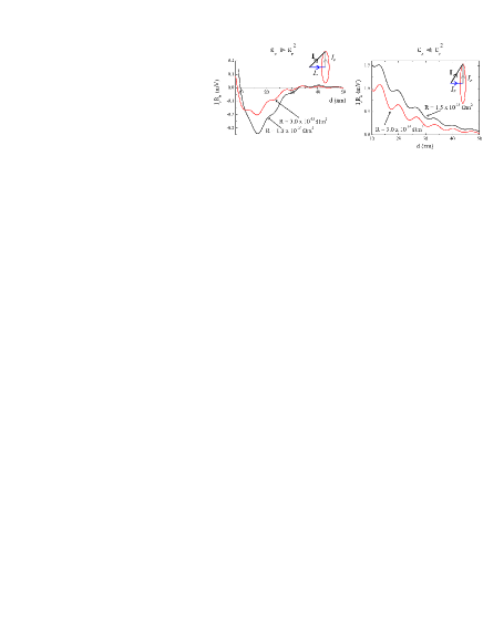
Figure 2: (Color online) Typical $I_{c}R_{n}$ dependence on the thickness $d$ of the FM layer ($\Delta=$ 2.2$\times$10^-22 J, $Q=$ 9 $\times$10⁸ m^-1, $D_{f}=$ 6 $\times$10^-4 m²s^-1, $D_{s}=$ 2.5 $\times$10^-4 m²s^-1, $\sigma_{f}=$ 4 $\times$10⁶ ($\Omega$m)^-1, $\sigma_{s}=$ 6 $\times$10⁶ ($\Omega$m)^-1): (left) in the limit of $\epsilon_{z}\gg\epsilon_{r}^{2}$ ($I_{r}/k_{B}=I_{z}/k_{B}=$ 100 K) and (right) in the limit of $\epsilon_{z}\ll\epsilon_{r}^{2}$ ($I_{r}/k_{B}=$ 130 K, $I_{z}/k_{B}<$ 4 K) for two different values of the interfacial resistance $R$.

Assuming that $\gamma_{b}\gg\max(1,\gamma)$ is true, the rigid boundary conditions are ReviewBuzd2005

$$\hat{F}_{L}=G_{s}\hat{F}(0)-\gamma_{B}\xi_{f}\frac{d\hat{F}(0)}{dz}$$ (26)

at the left side of the FM ($z=0$) and

$$\hat{F}_{R}=G_{s}\hat{F}(d)+\gamma_{B}\xi_{f}\frac{d\hat{F}(d)}{dz}$$ (27)

at the right side of the FM ($z=d$). If the FM layer is thick enough ($d\gg\xi_{f}$), the terms containing $e^{-K_{n}(d-z)}$ can be neglected from the general solution (24) near $z=0$, while the terms containing $e^{-K_{n}z}$ can be neglected near $z=d$. In this case we can take the components $f_{0}$, $f_{z}$ and $f_{\pm}$ of Eq. (24) at $z=d$ and obtain equations for the amplitudes $C_{n}$:

$$\frac{\Delta}{\hbar\omega}e^{i\Phi/2}=\sum_{n=1}^{4}C_{n}A_{n0}(1+\Gamma K_{n}),$$ (28)

$$0=\sum_{n=1}^{4}C_{n}A_{nz}(1+\Gamma K_{n}),$$ (29)

$$0=\sum_{n=1}^{4}C_{n}A_{n\pm}(1+\Gamma(K_{n}\pm iQ)),$$ (30)

where the notation $\Gamma=\gamma_{B}\xi_{f}/G_{s}$ is used. Similar equations hold for the amplitudes $B_{n}$ at $z=0$, the only difference is that the sign of the phase $\Phi/2$ in the first term of Eq. (28) is negative. Substituting $K_{n}$ and $A_{n\pm}$ into Eq. (30) and using $|K_{3,4}|\ll Q$ yields

$$(C_{1,2}-i\epsilon_{r}(C_{3}+C_{4}))+\Gamma(\pm Q\epsilon_{r}(C_{3}+C_{4})+k_{0}C_{1,2})=0,$$ (31)

where $k_{0}=Q\sqrt{2\epsilon_{\omega}+2\epsilon_{r}^{2}}$. Even though $\Gamma Q\gg 1$, $\Gamma Q\epsilon_{r}\ll 1$ for realistic values of the interfacial resistance; it follows from Eq. (31) that $C_{1},C_{2}\ll C_{3},C_{4}$, therefore the terms containing $C_{1}$ and $C_{2}$ can be neglected from Eqs. (28) and (29). Those equations with $A_{30}=A_{40}=1$ take the form of

$$\frac{\Delta}{\hbar\omega}e^{i\Phi/2}=(C_{3}+C_{4})+\Gamma(K_{3}C_{3}+K_{4}C_{4}),$$ (32)

$$0=(A_{3z}C_{3}+A_{4z}C_{4})+\Gamma(A_{3z}K_{3}C_{3}+A_{4z}K_{4}C_{4}).$$ (33)

In the following we work in the limit of $\epsilon_{z}\gg\epsilon_{r}^{2}$, so we take $A_{3z}$ and $A_{4z}$ given by Eq. (22) to get

$$C_{3,4}=\frac{\Delta e^{i\Phi/2}}{2\hbar\omega(1+K_{3,4}\Gamma)}\bigg{(}1\mp i\frac{\epsilon_{r}^{2}}{\epsilon_{z}}\bigg{)},$$ (34)

where the expression (20) for the roots $K_{3,4}$ can be approximated as $K_{3,4}\approx Q\sqrt{2\epsilon_{\omega}+2\epsilon_{r}^{2}\pm 2i\epsilon_{z}}$ in this case. Substituting $C_{3}$ and $C_{4}$ into Eq. (31) gives the remaining two amplitudes,

$$C_{1,2}=\frac{\Delta e^{i\Phi/2}\epsilon_{r}(i\mp\Gamma Q)}{2\hbar\omega(1+k_{0}\Gamma)}\bigg{(}\frac{1-i\epsilon_{r}^{2}/\epsilon_{z}}{1+K_{3}\Gamma}+\frac{1+i\epsilon_{r}^{2}/\epsilon_{z}}{1+K_{4}\Gamma}\bigg{)}.$$ (35)

The term $i$ can be neglected from the numerator, because $\Gamma Q\gg 1$. Furthermore, since $K_{3}$ and $K_{4}$ are complex conjugates if $\epsilon_{z}>\epsilon_{r}^{2}$, the sum in Eq. (35) can be simplified to

$$C_{1,2}=\mp\frac{\Delta e^{i\Phi/2}\epsilon_{r}\Gamma Q}{\hbar\omega(1+k_{0}\Gamma)}\mathrm{Re}\bigg{(}\frac{1-i\epsilon_{r}^{2}/\epsilon_{z}}{1+K_{3}\Gamma}\bigg{)}.$$ (36)

The results for $B_{3,4}$ and $B_{1,2}$ are the same as those given by Eqs. (34) and (36) with the only difference being a minus sign before $i\Phi/2$ in the phase factor of $\Delta$.

The Josephson current in the S/FM/S junction of area $A$ is given by Houzet2007

$$I=\frac{\pi\sigma_{f}A}{e}k_{B}T\sum_{\omega>0}\mathrm{Im}\Big{[}\mathrm{Tr}\Big{(}\hat{F}^{*}(z)\hat{\sigma}_{y}\frac{d\hat{F}(z)}{dz}\hat{\sigma}_{y}\Big{)}\Big{]},$$ (37)

which can be evaluated in the range $0<z<d$. We can substitute the solution (24) into Eq. (37) and take $z=d$; most terms do not give any imaginary contribution to the trace, hence we obtain

$$I=\frac{\pi\sigma_{f}A}{e}k_{B}T\sum_{\omega>0}\mathrm{Im}(S_{1}+S_{2}),$$ (38)

$$S_{1} = 2\sum_{0,z}\Big{(}\sum_{n=1}^{4}B_{n}^{*}A_{n(0,z)}^{*}e^{-K_{n}^{*}d}\sum_{n=1}^{4}C_{n}A_{n(0,z)}K_{n}$$ (39)

$$- \sum_{n=1}^{4}C_{n}^{*}A_{n(0,z)}^{*}\sum_{n=1}^{4}B_{n}A_{n(0,z)}K_{n}e^{-K_{n}d}\Big{)},$$

$$S_{2} = -\sum_{\pm}\Big{(}\sum_{n=1}^{4}B_{n}^{*}A_{n\mp}^{*}e^{-K_{n}^{*}d}\sum_{n=1}^{4}C_{n}A_{n\pm}(K_{n}\pm iQ)$$ (40)

$$- \sum_{n=1}^{4}C_{n}^{*}A_{n\mp}^{*}\sum_{n=1}^{4}B_{n}A_{n\pm}(K_{n}\pm iQ)e^{-K_{n}d}\Big{)}.$$

The first term $S_{1}$ mainly contains the solutions corresponding to the eigenvalues $K_{3,4}$, while the second term $S_{2}$ is mainly contributed by the solutions corresponding to $K_{1,2}$. By using the values of $A_{n0}$, $A_{nz}$ and $A_{n\pm}$ in the limit $\epsilon_{z}\gg\epsilon_{r}^{2}$, the expressions for $S_{1}$ and $S_{2}$ become

$$S_{1} = 4K_{3}e^{-K_{3}d}\bigg{(}1+i\frac{\epsilon_{r}^{2}}{\epsilon_{z}}\bigg{)}(B_{4}^{*}C_{3}-C_{4}^{*}B_{3})$$ (41)

$$+ 4K_{4}e^{-K_{4}d}\bigg{(}1-i\frac{\epsilon_{r}^{2}}{\epsilon_{z}}\bigg{)}(B_{3}^{*}C_{4}-C_{3}^{*}B_{4}),$$

$$S_{2}=4k_{0}\big{[}e^{-K_{1}d}(C_{2}^{*}B_{1}-B_{2}^{*}C_{1})+e^{-K_{2}d}(C_{1}^{*}B_{2}-B_{1}^{*}C_{2})\big{]}$$ (42)

in the main approximation. Here we neglected the terms containing the small amplitudes $A_{10}$, $A_{20}$, $A_{3\pm}$, $A_{4\pm}$ and used the fact that $|A_{3z}|=|A_{4z}|=1$ if $\epsilon_{z}>\epsilon_{r}^{2}$. By taking $K_{2}=K_{1}^{*}$ and $K_{4}=K_{3}^{*}$ into account, then putting the above obtained expressions for $B_{n}$ and $C_{n}$ into Eqs. (41) and (42) we obtain

$$S_{1}=4i\sin(\Phi)\frac{\Delta^{2}}{\hbar^{2}\omega^{2}}\mathrm{Re}\bigg{[}\frac{K_{3}e^{-K_{3}d}}{(1+K_{3}\Gamma)^{2}}\bigg{(}1-i\frac{\epsilon_{r}^{2}}{\epsilon_{z}}\bigg{)}\bigg{]},$$ (43)

$$S_{2} = 16i\sin(\Phi)\frac{\Delta^{2}}{\hbar^{2}\omega^{2}}\bigg{[}\mathrm{Re}\bigg{(}\frac{1-i\epsilon_{r}^{2}/\epsilon_{z}}{1+K_{3}\Gamma}\bigg{)}\bigg{]}^{2}$$ (44)

$$\times\frac{\epsilon_{r}^{2}Q^{2}\Gamma^{2}k_{0}e^{-k_{0}d}}{(1+k_{0}\Gamma)^{2}}\cos(Qd).$$

The Josephson current through the S/FM/S junction therefore obeys the formula $I=I_{c}\sin(\Phi)$, where the critical current $I_{c}$ is given by

$$I_{c}R_{n}=4\pi k_{B}T\frac{d+2\xi_{f}\gamma_{B}}{e}\sum_{\omega>0}\frac{\Delta^{2}}{\hbar^{2}\omega^{2}}\Bigg{[}\mathrm{Re}\bigg{[}\frac{K_{3}e^{-K_{3}d}}{(1+K_{3}\Gamma)^{2}}\bigg{(}1-i\frac{\epsilon_{r}^{2}}{\epsilon_{z}}\bigg{)}\bigg{]}+\bigg{[}\mathrm{Re}\bigg{(}\frac{1-i\epsilon_{r}^{2}/\epsilon_{z}}{1+K_{3}\Gamma}\bigg{)}\bigg{]}^{2}\frac{4\epsilon_{r}^{2}Q^{2}\Gamma^{2}k_{0}e^{-k_{0}d}}{(1+k_{0}\Gamma)^{2}}\cos(Qd)\Bigg{]}$$ (45)

with $R_{n}=(d+2\xi_{f}\gamma_{B})/\sigma_{f}A$ being the normal state resistance of the junction.

The dependence of $I_{c}R_{n}$ on the thickness $d$ predicted by Eq. (45) is plotted in Fig. 2 (left) for two values of the interfacial resistance $R$. Both curves show a small, rapid oscillation superimposed on a large, slow oscillation; they both decay on the scale of the slow oscillation. Comparison between the two curves demonstrates that an increase in $R$ reduces the current, but makes the rapid oscillations relatively more pronounced.

The first term in Eq. (45) gives the slow oscillation, which is mainly due to the “short-range” singlet and triplet components of the anomalous Green’s function $\hat{F}$ (i.e. the singlet component $f_{0}$ and the triplet component $f_{z}$ with zero projection on the $z$ axis). Conversely, the second term in Eq. (45) corresponds to the rapid oscillation, which is related to the “long-range” triplet components (i.e. the triplet components $f_{\pm}$ with projection $\pm 1$ on the $z$ axis). Note that in our case the terms “short-range” and “long-range” do not mean any difference in the respective decaying lengths; they are only defined like this to be consistent with the notions used in other papers. Volkov2006 ; Houzet2007

Unlike the slow oscillation which is also present in a system with a homogeneous FM, the rapid oscillation appears as a direct consequence of the inhomogeneous magnetization. This is shown clearly by the coincidence of its oscillation period and the magnetic spiral wavelength $\lambda$. The magnetization changes quickly with respect to the FM coherence length $\xi_{f}$, which explains why the amplitude of the rapid oscillation is small compared to that of the slow oscillation.

By taking the limit of $I_{r}\rightarrow$ 0 (and hence $\epsilon_{r}\rightarrow$ 0), we recover an S/FM/S junction with a homogeneous FM of exchange energy $I_{z}$. In this limit, Eq. (45) reduces to

$$I_{c}R_{n}=4\pi k_{B}T\frac{d+2\xi_{f}\gamma_{B}}{e}\sum_{\omega>0}\frac{\Delta^{2}}{\hbar^{2}\omega^{2}}\mathrm{Re}\bigg{[}\frac{K_{3}e^{-K_{3}d}}{(1+K_{3}\Gamma)^{2}}\bigg{]}$$ (46)

with the root $K_{3}$ taking the form of

$$K_{3}=\sqrt{2k_{\omega}^{2}+2ik_{z}^{2}}.$$ (47)

This is the standard formula for $I_{c}R_{n}$ in a Josephson junction with a homogeneous FM weak link. ReviewBuzd2005

The same result is obtained in the limit of $Q\rightarrow\infty$ because $\epsilon_{r}=k_{r}^{2}/Q^{2}\rightarrow$ 0 in this case. The amplitude of the rapid oscillation vanishes as $Q^{-2}$, and hence we recover Eq. (46). This is physically understandable; as the FM coherence length becomes very much larger than the characteristic spiral wavelength, the radial magnetization “averages out” on the scale of $\xi_{f}$, which means that the situation is equivalent to $I_{r}\rightarrow$ 0.

Now we can return to Eqs. (32) and (33) and take the opposite limit, i.e. where $\epsilon_{z}\ll\epsilon_{r}^{2}$. In this case we use $A_{3z}$ and $A_{4z}$ given by Eq. (23) to obtain different values for the amplitudes $B_{n}$ and $C_{n}$. However, the expression (38) with the same terms $S_{1}$ and $S_{2}$ still holds for the Josephson current. After substituting the new values of $B_{n}$ and $C_{n}$ into Eq. (38) and taking approximations valid in the given limit, we recover $I=I_{c}\sin(\Phi)$ and obtain

$$I_{c}R_{n}=4\pi k_{B}T\frac{d+2\xi_{f}\gamma_{B}}{e}\sum_{\omega>0}\frac{\Delta^{2}}{\hbar^{2}\omega^{2}}\Bigg{[}\bigg{[}\frac{K_{3}e^{-K_{3}d}}{(1+K_{3}\Gamma)^{2}}-\frac{\epsilon_{z}^{2}}{4\epsilon_{r}^{4}}\frac{K_{4}e^{-K_{4}d}}{(1+K_{4}\Gamma)^{2}}\bigg{]}+\frac{4\epsilon_{r}^{2}Q^{2}\Gamma^{2}k_{0}e^{-k_{0}d}}{(1+k_{0}\Gamma)^{2}(1+K_{3}\Gamma)^{2}}\cos(Qd)\Bigg{]}$$ (48)

for the critical current. The roots $K_{3,4}$ given by Eq. (20) can be approximated as $K_{3}\approx Q\sqrt{2\epsilon_{\omega}+4\epsilon_{r}^{2}}$ and $K_{4}\approx Q\sqrt{2\epsilon_{\omega}}$ if $\epsilon_{z}\ll\epsilon_{r}^{2}$.

The $I_{c}R_{n}$ dependence on $d$ as given by Eq. (48) is represented in Fig. 2 (right). The rapid oscillation is similar as in the limit of $\epsilon_{z}\gg\epsilon_{r}^{2}$, but the slow oscillation is absent; the other component of $I_{c}$ decays exponentially without oscillation. The rapid oscillation is still related to the “long-range” triplet components, whereas the exponential decay is to the “short-range” singlet and triplet components.

In the case between the two limits (where $\epsilon_{z}\sim\epsilon_{r}^{2}$), both expressions (45) and (48) are applicable, but they are not as accurate as when they are used in their respective limiting cases. Since the approximations leading to Eq. (45) are less sensitive than those required for Eq. (48), the former is preferred to be used in such a case.

V Computational method for calculating the Josephson current

In this section we describe an alternative method for obtaining the Josephson current in the S/FM/S junction; it requires computational power and does not yield an analytical formula, but is exact within the framework of the linearized Usadel equations. The basic steps are the same as in the previous sections: we first solve the linearized Usadel equation (2) with the boundary conditions [Eqs. (26) and (27)], then evaluate Eq. (37) at a suitable location.

Let us introduce the formal vector

$$\mathbf{F}(z)=\Big{(}f_{0},f_{x},f_{y},f_{z},\frac{df_{0}}{dz},\frac{df_{x}}{dz},\frac{df_{y}}{dz},\frac{df_{z}}{dz}\Big{)}$$ (49)

containing the components of $\hat{F}$ and their respective derivatives with respect to $z$. We denote the value of this vector $\mathbf{F}_{L}$ at the right side of the left S (at $z=0$) and $\mathbf{F}_{R}$ at the left side of the right S (at $z=d$). These consist of the components of $\hat{F}_{L}$ and $\hat{F}_{R}$, respectively. By using the method described in the Appendix, we can relate $\mathbf{F}_{L}$ and $\mathbf{F}_{R}$ through a matrix type equation. Since we know the first four components of both $\mathbf{F}_{L}$ and $\mathbf{F}_{R}$, we can use this equation to obtain the remaining four components (the derivatives).

The Josephson current is evaluated with Eq. (37) in the S side of the left S/FM interface; since we calculate the current in the S, we must substitute $\sigma_{s}$ instead of $\sigma_{f}$ in Eq. (37). By using $f_{xL}=f_{yL}=f_{zL}=0$ the formula simplifies to

$$I=\frac{2\pi\sigma_{s}A}{e}k_{B}T\sum_{\omega>0}\mathrm{Im}\bigg{(}f_{0L}\frac{df_{0L}}{dz}\bigg{)},$$ (50)

where $f_{0L}=\Delta e^{-i\Phi/2}/\sqrt{\Delta^{2}+\hbar^{2}\omega^{2}}$ and $df_{0L}/dz$ is calculated by the method described in the Appendix. By setting the phase difference to $\Phi=\pi/2$ we obtain

$$I_{c}R_{n}=2\pi k_{B}T\frac{\sigma_{s}(d+2\xi_{f}\gamma_{B})}{e\sigma_{f}}\sum_{\omega>0}\mathrm{Im}\bigg{(}f_{0L}\frac{df_{0L}}{dz}\bigg{)}.$$ (51)

Note that the values of $f_{0L}$ and $df_{0L}/dz$ depend on the phase difference $\Phi$, as well as on other parameters describing the junction.

Evaluating $df_{0L}/dz$ requires inverting matrices and taking matrix exponentials, therefore this method does not give an analytical formula like expressions (45) and (48). On the other hand, it gives the right result in the more general case, even if $Q$ is not large [in which case neither Eq. (45), nor Eq. (48) is applicable]. This method can also be used to check analytical results; in our case it seems that within their respective ranges, Eqs. (45) and (48) show good coincidence with the results obtained by the computational method: see Fig. 3.

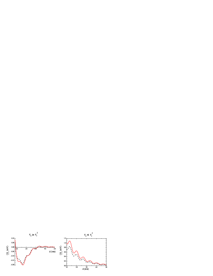
Figure 3: (Color online) Comparison of the analytical (solid curve) and computational (dashed curve) results for $I_{c}R_{n}$ in the function of the thickness $d$: (left) in the limit of $\epsilon_{z}\gg\epsilon_{r}^{2}$ and (right) in the limit of $\epsilon_{z}\ll\epsilon_{r}^{2}$. The parameters used are identical to those in Fig. 2 with $R=$ 3.0$\times$10^-15 $\Omega$ m².

VI Summary

We have calculated the Josephson current in a superconductor/ferromagnetic/superconductor junction in which the ferromagnet has a conical magnetic structure. In view of the realistic interfaces that can exist between thin-film superconductors (Al, Pb, and Nb being the elements typically used) and thin films of conical magnets such as Ho, we have extended the problem to a regime in which the ferromagnetic coherence length is long compared to the electron mean-free path and the normalized spiral length of the magnetic spiral.

From the materials point of view, the dirty-limit model we present is physically reasonable and most applicable for when the Ho thin film is polycrystalline. The electron mean-free path of thin film Ho is $<$ 1.0 nm and its normalized spiral length is $\sim$ 1.1 nm, whereas the coherence length in such films has recently been determined to be in the 6$-$7 nm range.Ho5

In this new situation, we have shown that the Josephson current is highly sensitive to the length of the conical ferromagnet $\lambda$ with the current containing a rapidly oscillating component in the function of the total conical magnetic thickness. These rapid oscillations are superimposed on a much slower oscillation which has a longer wavelength. The longer oscillation is directly linked to the strength of the ferromagnetic component and mainly depends on the singlet part of the anomalous Green’s function $\hat{F}$. The sign of the longer oscillation varies with multiple phase transitions from $0$ to $\pi$ which depend on the thickness of the magnetic layer. The rapid oscillations are linked to the triplet components $f_{\pm}$ of the anomalous Green’s function $\hat{F}$. Although of a shorter wavelength to the slower oscillations, this rapid oscillation also decays on the scale of the magnetic coherence length.

The main feature of the results presented in this paper is that the Josephson coupling through a conical ferromagnet may not be long ranged as previously expected. In the limit considered, we have shown that the proximity effect is short with a length scale comparable to that of the proximity effects in a weak and collinear ferromagnet. Thus, the theory explained in this paper is complementary to previous studiesLinder2009 ; Sosnin2006 ; Volkov2006 which assume that the magnetism of thin-film conical magnets is comparable to the magnetism of conical magnets in bulk single-crystal form.

From the experimental view, the theory presented in this paper is directly applicable to situations in which two singlet-type superconductors are coupled via a rare-earth conical magnet (e.g., Ho). The experiment should be designed in such a way that the current flowing through the superconductor/ferromagnetic/superconductor junction is restricted to the growth direction of the conical magnet, e.g., along the z axis, such as in the case illustrated in Fig. 1(a). For similar experimental situations, see references ZeroPi5 and Bell2003 .

*

Appendix A Computational method in detail

The boundary conditions at the S/FM interfaces are given by Eqs. (26) and (27), and the equations relating the appropriate derivatives,

$$G_{s}\frac{d\hat{F}_{L}}{dz}=\frac{\sigma_{f}}{\sigma_{s}}\frac{d\hat{F}(0)}{dz}\quad\textrm{and}\quad\frac{\sigma_{f}}{\sigma_{s}}\frac{d\hat{F}(d)}{dz}=G_{s}\frac{d\hat{F}_{R}}{dz}.$$ (52)

If we assume rigid boundary conditions, $d\hat{F}_{L}/dz$ and $d\hat{F}_{R}/dz$ are small because $\hat{F}_{L},\hat{F}_{R}\approx$ constant. However, they are still not equal to zero and they must not be neglected in this treatment. The boundary conditions (26), (27) and (52) can be written as vector equations: $\mathbf{F}(0)=\mathbf{\hat{M}}_{fL}\mathbf{F}_{L}$ and $\mathbf{F}_{R}=\mathbf{\hat{M}}_{Rf}\mathbf{F}(d)$ with the 8$\times$8 matrices

$$\mathbf{\hat{M}}_{fL}=\left(\begin{array}[]{cc}G_{s}^{-1}\hat{1}&R\sigma_{s}\hat{1}\\ \hat{0}&G_{s}\sigma_{s}\hat{1}/\sigma_{f}\end{array}\right),$$ (53)

$$\mathbf{\hat{M}}_{Rf}=\left(\begin{array}[]{cc}G_{s}\hat{1}&R\sigma_{f}\hat{1}\\ \hat{0}&G_{s}^{-1}\sigma_{f}\hat{1}/\sigma_{s}\end{array}\right).$$ (54)

The symbols $\hat{1}$ and $\hat{0}$ denote the 4$\times$4 unit and zero matrices, respectively. In order to deal with the interior of the FM, we return to Eqs. (6)$-$(8) and introduce new functions as $f_{+}=f_{+}^{\prime}e^{iQz}$ and $f_{-}=f_{-}^{\prime}e^{-iQz}$ (primes do not denote derivatives here). In this case we obtain the equations

$$\frac{d^{2}f_{0}}{dz^{2}}-2k_{\omega}^{2}f_{0}-2ik_{z}^{2}f_{z}-ik_{r}^{2}(f_{+}^{\prime}+f_{-}^{\prime})=0,$$ (55)

$$\frac{d^{2}f_{\pm}^{\prime}}{dz^{2}}\pm 2iQ\frac{df_{\pm}^{\prime}}{dz}-Q^{2}f_{\pm}^{\prime}-2k_{\omega}^{2}f_{\pm}^{\prime}-2ik_{r}^{2}f_{0}=0,$$ (56)

$$\frac{d^{2}f_{z}}{dz^{2}}-2k_{\omega}^{2}f_{z}-2ik_{z}^{2}f_{0}=0.$$ (57)

Equations (55)$-$(57) can be written compactly as

$$\frac{d\mathbf{F}^{\prime}(z)}{dz}=\mathbf{\hat{M}}_{F}\mathbf{F}^{\prime}(z)\quad\textrm{with}\quad\mathbf{\hat{M}}_{F}=\left(\begin{array}[]{cc}\hat{0}&\hat{1}\\ \hat{K}&\hat{L}\end{array}\right)$$ (58)

if we introduce the formal vector

$$\mathbf{F}^{\prime}(z)=\Big{(}f_{0},f_{+}^{\prime},f_{-}^{\prime},f_{z},\frac{df_{0}}{dz},\frac{df_{+}^{\prime}}{dz},\frac{df_{-}^{\prime}}{dz},\frac{df_{z}}{dz}\Big{)}.$$ (59)

The 4$\times$4 matrices $\hat{K}$ and $\hat{L}$ are given by

$$\hat{K}=\left(\begin{array}[]{cccc}2k_{\omega}^{2}&ik_{r}^{2}&ik_{r}^{2}&2ik_{z}^{2}\\ 2ik_{r}^{2}&Q^{2}+2k_{\omega}^{2}&0&0\\ 2ik_{r}^{2}&0&Q^{2}+2k_{\omega}^{2}&0\\ 2ik_{z}^{2}&0&0&2k_{\omega}^{2}\end{array}\right),$$ (60)

$$\hat{L}=\left(\begin{array}[]{cccc}0&0&0&0\\ 0&-2iQ&0&0\\ 0&0&2iQ&0\\ 0&0&0&0\end{array}\right),$$ (61)

as it is clear from Eqs. (55)$-$(57). Solving Eq. (58) in the region $0<z<d$ gives $\mathbf{F}^{\prime}(d)=\exp(d\mathbf{\hat{M}}_{F})\mathbf{F}^{\prime}(0)$. We also introduce the conversion matrices

$$\mathbf{\hat{M}}_{Ff}=\left(\begin{array}[]{cccccccc}1&0&0&0&0&0&0&0\\ 0&1&i&0&0&0&0&0\\ 0&1&-i&0&0&0&0&0\\ 0&0&0&1&0&0&0&0\\ 0&0&0&0&1&0&0&0\\ 0&-iQ&Q&0&0&1&i&0\\ 0&iQ&Q&0&0&1&-i&0\\ 0&0&0&0&0&0&0&1\end{array}\right),$$ (62)

$$\mathbf{\hat{M}}_{fF}=\left(\begin{array}[]{cccccccc}1&0&0&0&0&0&0&0\\ 0&\alpha/2&1/2\alpha&0&0&0&0&0\\ 0&-i\alpha/2&i/2\alpha&0&0&0&0&0\\ 0&0&0&1&0&0&0&0\\ 0&0&0&0&1&0&0&0\\ 0&i\alpha Q/2&-iQ/2\alpha&0&0&\alpha/2&1/2\alpha&0\\ 0&\alpha Q/2&Q/2\alpha&0&0&-i\alpha/2&i/2\alpha&0\\ 0&0&0&0&0&0&0&1\end{array}\right),$$ (63)

where $\alpha=e^{iQd}$. These can be used to convert $\mathbf{F}(0)$ to $\mathbf{F}^{\prime}(0)$ as $\mathbf{F}^{\prime}(0)=\mathbf{\hat{M}}_{Ff}\mathbf{F}(0)$ and $\mathbf{F}^{\prime}(d)$ to $\mathbf{F}(d)$ as $\mathbf{F}(d)=\mathbf{\hat{M}}_{fF}\mathbf{F}^{\prime}(d)$. By taking the matrices defined in Eqs. (53), (54), (58), (62) and (63) we obtain

$$\mathbf{F}_{R}=\mathbf{\hat{M}}\mathbf{F}_{L},$$ (64)

$$\mathbf{\hat{M}}=\mathbf{\hat{M}}_{Rf}\mathbf{\hat{M}}_{fF}\exp(d\mathbf{\hat{M}}_{F})\mathbf{\hat{M}}_{Ff}\mathbf{\hat{M}}_{fL}.$$ (65)

Due to rigid boundary conditions, the components of $\hat{F}_{L}$ are $f_{0L}=\Delta e^{-i\Phi/2}/\sqrt{\Delta^{2}+\hbar^{2}\omega^{2}}$ and $f_{xL}=f_{yL}=f_{zL}=0$, while the components of $\hat{F}_{R}$ are $f_{0R}=\Delta e^{i\Phi/2}/\sqrt{\Delta^{2}+\hbar^{2}\omega^{2}}$ and $f_{xR}=f_{yR}=f_{zR}=0$. The first four components of the vectors $\mathbf{F}_{L}$ and $\mathbf{F}_{R}$ are therefore known and Eq. (64) can be used to obtain the remaining four components (the derivatives). If we divide the matrix $\mathbf{\hat{M}}$ into 4$\times$4 blocks as

$$\mathbf{\hat{M}}=\left(\begin{array}[]{cc}\hat{M}_{11}&\hat{M}_{12}\\ \hat{M}_{21}&\hat{M}_{22}\end{array}\right),$$ (66)

and then take the first four components of Eq. (64), a pre-multiplication by $\hat{M}_{12}^{-1}$ gives the derivatives as

$$\left(\begin{array}[]{c}df_{0L}/dz\\ df_{xL}/dz\\ df_{yL}/dz\\ df_{zL}/dz\end{array}\right)=\hat{M}_{12}^{-1}\Bigg{[}\left(\begin{array}[]{c}f_{0R}\\ f_{xR}\\ f_{yR}\\ f_{zR}\end{array}\right)-\hat{M}_{11}\left(\begin{array}[]{c}f_{0L}\\ f_{xL}\\ f_{yL}\\ f_{zL}\end{array}\right)\Bigg{]}.$$ (67)

The first component $df_{0L}/dz$ is used in Eqs. (50) and (51).

References

• (1) A. I. Buzdin, Rev. Mod. Phys. 77, 935 (2005).
• (2) F. S. Bergeret, A. F. Volkov and K. B. Efetov, Phys. Rev. B 64, 134506 (2001).
• (3) F. S. Bergeret, A. F. Volkov and K. B. Efetov, Rev. Mod. Phys. 77, 1321 (2005).
• (4) J. S. Jiang, D. Davidović, Daniel H. Reich, and C. L. Chien, Phys. Rev. Lett. 74, 314 (1995).
• (5) Th. Mühge, N. N. Garif’yanov, Yu. V. Goryunov, G. G. Khaliullin, L. R. Tagirov, K. Westerholt, I. A. Garifullin, and H. Zabel, Phys. Rev. Lett. 77, 1857 (1996).
• (6) M. Vélez, M. C. Cyrille, S. Kim, J. L. Vicent, Ivan K. Schuller, Phys. Rev. B 59, 14659 (1999).
• (7) P. Koorevaar, Y. Suzuki, R. Coehoorn, J. Aarts, Phys. Rev. B 49, 441 (1994).
• (8) V. Pen̋a, Z. Sefrioui, D. Arias, C. Leon, J. Santamaria, J. L. Martinez, S. G. E. te Velthuis, and A. Hoffmann, Phys. Rev. Lett. 94, 057002 (2005).
• (9) I. C. Moraru, W. P. Pratt, Jr., and N. O. Birge, Phys. Rev. Lett. 96, 037004 (2006).
• (10) A. Yu. Rusanov, S. Habraken, and J. Aarts, Phys. Rev. B 73, 060505(R) (2006).
• (11) J. Y. Gu, C.-Y. You, J. S. Jiang, J. Pearson, Ya. B. Bazaliy, and S. D. Bader, Phys. Rev. Lett. 89, 267001 (2002).
• (12) A. Potenza and C. H. Marrows, Phys. Rev. B 71, 180503(R) (2005).
• (13) D. Stamopoulos, E. Manios, and M. Pissas, Phys. Rev. B 75, 014501 (2007).
• (14) V. V. Ryazanov, V. A. Oboznov, A. Yu. Rusanov, A. V. Veretennikov, A. A. Golubov, and J. Aarts, Phys. Rev. Lett. 86, 2427 (2001).
• (15) T. Kontos, M. Aprili, J. Lesueur, F. Genêt, B. Stephanidis, and R. Boursier, Phys. Rev. Lett. 89, 137007 (2002).
• (16) C. Bell1, R. Loloee, G. Burnell, and M. G. Blamire, Phys. Rev.B 71, 180501 (2005).
• (17) V. A. Oboznov, V. V. Bol’ginov, A. K. Feofanov, V. V. Ryazanov, and A. I. Buzdin, Phys. Rev. Lett. 96, 197003 (2006).
• (18) J. W. A. Robinson, S. Piano, G. Burnell, C. Bell, and M. G. Blamire, Phys. Rev. Lett. 97, 177003 (2006).
• (19) F.S. Bergeret, A.F. Volkov, and K. B. Efetov, Phys. Rev. Lett. 86, 4096 (2001)
• (20) A. Yu. Aladyshkin, A. I. Buzdin, A. A. Fraerman, A. S. Melnikov, D. A. Ryzhov, and A. V. Sokolov, Phys. Rev. B 68, 184508 (2003).
• (21) Z. Yang, M. Lange, A. Volodin, R. Szymczak and V. V. Moshchalkov, Nature Mater. 3, 793 (2004).
• (22) W. Gillijns, A. Yu. Aladyshkin, M. Lange, M. J. Van Bael, and V. V. Moshchalkov, Phys. Rev. Lett. 95, 227003 (2005).
• (23) L. Y. Zhu, T. Y. Chen, and C. L. Chien, Phys. Rev. Lett. 101, 017004 (2008).
• (24) A. F. Volkov and K. B. Efetov, Phys. Rev. B 78, 024519 (2008).
• (25) A. I. Buzdin and A. S. Melnikov, Phys. Rev. B 67, 020503 (2003).
• (26) T. S. Khaire, W. P. Pratt, Jr., and N. O. Birge, Phys. Rev. B 79, 094523 (2009).
• (27) Yu. S. Barash, I. V. Bobkova, and T. Kopp, Phys. Rev. B 66, 140503(R) (2002).
• (28) T. Yu. Karminskaya, M. Yu. Kupriyanov, and A. A. Golubov, JETP Lett. 87, 570 (2008).
• (29) V. N. Krivoruchko and E. A. Koshina, Phys. Rev. B 64, 172511 (2001).
• (30) A. F. Volkov, F. S. Bergeret, and K. B. Efetov, Phys. Rev. Lett. 90, 117006 (2003).
• (31) A. Vedyayev, C. Lacroix, N. Pugach and N. Ryzhanova, Europhys. Lett. 71, 679 (2005).
• (32) C. Bell, G. Burnell, C. W. Leung, E. J. Tarte, D.-J. Kang, and M. G. Blamire, Appl. Phys. Lett. 84, 1153(2004).
• (33) P. Cadden-Zimansky, Ya. B. Bazaliy, L. M. Litvak, J. S. Jiang, J. Pearson, J. Y. Gu, C.-Y. You, M. R. Beasley, and S. D. Bader, Phys. Rev. B 77, 184501 (2008).
• (34) J. W. A. Robinson, G. B. Halász, A. I. Buzdin and M. G. Blamire, arXiv:0808.0166 (unpublished).
• (35) M. Houzet and A. I. Buzdin, Phys. Rev. B 76, 060504(R) (2007).
• (36) J. Linder, T. Yokoyama, and P. Sudbø, Phys. Rev. B 79, 054523 (2009).
• (37) I. Sosnin, H. Cho, V. T. Petrashov, and A. F. Volkov, Phys. Rev. Lett. 96, 157002 (2006).
• (38) A. F. Volkov, A. Anishchanka, and K. B. Efetov, Phys. Rev. B 73, 104412 (2006).
• (39) M. Eschrig and T. Löfwander, Nature Phys. 4, 138 (2008).
• (40) M. Eschrig, J. Kopu, J. C. Cuevas, and G. Schön, Phys. Rev. Lett. 90, 137003 (2003).
• (41) Y. Asano, Y. Sawa, Y. Tanaka, A. A. Golubov, Phys. Rev. B 76, 224525 (2007).
• (42) A. V. Galaktionov, M. S. Kalenkov, A. D. Zaikin, Phys. Rev. B 77, 094520 (2008).
• (43) R. S. Keizer, S. T. B. Goennenwein, T. M. Klapwijk, G. Miao, G. Xiao and A. Gupta, Nature (London) 439, 825 (2006).
• (44) W. C. Koehler, J. W. Cable, H. R. Child, M. K. Wilkinson, and E. O. Wollan, Phys. Rev. 158, 450 (1967).
• (45) S. Chikazumi, Physics of Ferromagnetism (Oxford University Press, England, 1997).
• (46) K. V. Rao , Phys. Rev. Lett. 22, 943 (1969).
• (47) J. Witt, S. Langridge, T. Hase, and M. G. Blamire (unpublished).
• (48) J. Witt, J. W. A. Robinson, and M. G. Blamire (unpublished).
• (49) C. Bell, G. Burnell, D.-J. Kang, R. H. Hadfield, M. J. Kappers, and M. G. Blamire, Nanotechnology 14, 630 (2003).