Semidefinite representation of
convex hulls of rational varieties

Abstract

Using elementary duality properties of positive semidefinite moment matrices and polynomial sum-of-squares decompositions, we prove that the convex hull of rationally parameterized algebraic varieties is semidefinite representable (that is, it can be represented as a projection of an affine section of the cone of positive semidefinite matrices) in the case of (a) curves; (b) hypersurfaces parameterized by quadratics; and (c) hypersurfaces parameterized by bivariate quartics; all in an ambient space of arbitrary dimension.

1 Introduction

Semidefinite programming, a versatile extension of linear programming to the convex cone of positive semidefinite matrices (semidefinite cone for short), has found many applications in various areas of applied mathematics and engineering, especially in combinatorial optimization, structural mechanics and systems control. For example, semidefinite programming was used in [6] to derive linear matrix inequality (LMI) convex inner approximations of non-convex semi-algebraic stability regions, and in [7] to derive a hierarchy of embedded convex LMI outer approximations of non-convex semi-algebraic sets arising in control problems.

It is easy to prove that affine sections and projections of the semidefinite cone are convex semi-algebraic sets, but it is still unknown whether all convex semi-algebraic sets can be modeled like this, or in other words, whether all convex semi-algebraic sets are semidefinite representable. Following the development of polynomial-time interior-point algorithms to solve semidefinite programs, a long list of semidefinite representable semi-algebraic sets and convex hulls was initiated in [10] and completed in [1]. Latest achievements in the field are reported in [8] and [5].

In this paper we aim at enlarging the class of semi-algebraic sets whose convex hulls are explicitly semidefinite representable. Using elementary duality properties of positive semidefinite moment matrices and polynomial sum-of-squares decompositions – nicely recently surveyed in [9] – we prove that the convex hull of rationally parameterized algebraic varieties is explicitly semidefinite representable in the case of (a) curves; (b) hypersurfaces parameterized by quadratics; and (c) hypersurfaces parameterized by bivariate quartics; all in an ambient space of arbitrary dimension.

Rationally parameterized surfaces arise often in engineering, and especially in computer-aided design (CAD). For example, the CATIA (Computer Aided Three-dimensional Interactive Application) software, developed since 1981 by the French company Dassault Systèmes, uses rationally parameterized surfaces as its core 3D surface representation. CATIA was originally used to develop Dassault’s Mirage fighter jet for the French airforce, and then it was adopted in aerospace, automotive, shipbuilding, and other industries. For example, Airbus aircrafts are designed in Toulouse with the help of CATIA, and architect Frank Gehry has used the software to design his curvilinear buildings, like the Guggenheim Museum in Bilbao or the Dancing House in Prague, near the Charles Square buildings of the Czech Technical University.

2 Notations and definitions

Let $x=[x_{0},\>x_{1},\>,\cdots,x_{m}]\in{\mathbb{R}}^{m+1}$ and

$$\zeta_{d}(x)=[x_{0}^{d},\>x_{0}^{d-1}x_{1},\>x_{0}^{d-1}x_{2},\>\cdots,x_{0}^{d-2}x_{1}^{2},\>\cdots,x_{m}^{d}]\in{\mathbb{R}}^{s(m,d)}[x]$$

denote a basis vector of $m$-variate forms of degree $d$, with $s(m,d)=(m+d)!/(m!d!)$. Let $y=[y_{\alpha}]_{|\alpha|\leq 2d}\in{\mathbb{R}}^{s(m,2d)}$ be a real-valued sequence indexed in basis $\zeta_{2d}(x)$, with $\alpha\in{\mathbb{N}}^{m}$ and $|\alpha|=\sum_{k}\alpha_{k}$. A form $x\mapsto p(x)=p^{T}\zeta_{2d}(x)$ is expressed in this basis via its coefficient vector $p\in{\mathbb{R}}^{s(m,2d)}$. Given a sequence $y\in{\mathbb{R}}^{s(m,2d)}$, define the linear mapping $p\mapsto L_{y}(p)=p^{T}y$, and the linear moment matrix $M_{d}(y)$ satisfying the relation $L_{y}(pq)=p^{T}M_{d}(y)q$ for all $p,q\in{\mathbb{R}}^{s(m,d)}$. It has entries $[M_{d}(y)]_{\alpha,\beta}=L_{y}([\zeta_{d}(x)\zeta_{d}(x)^{T}]_{\alpha,\beta})=y_{\alpha+\beta}$ for all $\alpha,\beta\in{\mathbb{N}}^{m}$, $|\alpha|+|\beta|\leq 2d$. For example, when $m=2$ and $d=2$ (trivariate quartics) we have $s(m,2d)=15$. To the form $p(x)=x_{0}^{4}-x_{0}x_{1}x_{2}^{2}+5x_{1}^{3}x_{2}$ we associate the linear mapping $L_{y}(p)=y_{00}-y_{12}+5y_{31}$. The 6-by-6 moment matrix is given by

$$M_{2}(y)=\left[\begin{array}[]{c|cc|ccc}y_{00}&*&*&*&*&*\\ \hline\cr y_{10}&y_{20}&*&*&*&*\\ y_{01}&y_{11}&y_{02}&*&*&*\\ \hline\cr y_{20}&y_{30}&y_{21}&y_{40}&*&*\\ y_{11}&y_{21}&y_{12}&y_{31}&y_{22}&*\\ y_{02}&y_{12}&y_{03}&y_{22}&y_{13}&y_{04}\end{array}\right]$$

where symmetric entries are denoted by stars. See [9] for more details on these notations and constructions.

Given a set $\mathcal{Z}$, let $\mathrm{conv}\>{\mathcal{Z}}$ denote its convex hull, the smallest convex set containing $\mathcal{Z}$. Finally, the notation $M_{d}(y)\succeq 0$ means that matrix $M_{d}(y)$ is positive semidefinite.

3 Convex cones and moment matrices

Consider the Veronese variety

$${\mathcal{W}}_{m,d}=\{\zeta_{2d}(x)\in{\mathbb{R}}^{s(m,2d)}\>:\>x\in{\mathbb{R}}^{m+1}\}$$

and the convex cones

$${\mathcal{Z}}_{m,d}={\mathrm{conv}\>}{\mathcal{W}}_{m,d}$$

and

$${\mathcal{Y}}_{m,d}=\{y\in{\mathbb{R}}^{s(m,2d)}\>:\>M_{d}(y)\succeq 0\}.$$

Theorem 1

If $m=1$ or $d=1$ or $d=m=2$ then ${\mathcal{Z}}_{m,d}={\mathcal{Y}}_{m,d}$.

Proof: The inclusion ${\mathcal{Z}}_{m,d}\subset{\mathcal{Y}}_{m,d}$ follows from the definition of a moment matrix since

$$M_{d}(\zeta_{2d}(x))=\zeta_{d}(x)\zeta_{d}(x)^{T}\succeq 0.$$

The converse inclusion is shown by contradiction. Assume that $y^{*}\notin{\mathcal{Z}}_{m,d}$ and hence that there exists a (strictly separating) hyperplane $\{y\>:p(y)=0\}$ such that $p^{T}y^{*}<0$ and $p^{T}y\geq 0$ for all $y\in{\mathcal{Z}}_{m,d}$. It follows that form $x\mapsto p(x)=p^{T}\zeta_{2d}(x)$ is globally non-negative. Since $m=1$ or $d=1$ or $d=m=2$, the form can be expressed as a sum of squares of forms [9, Theorem 3.4] and we can write $p(x)=\sum_{k}q_{k}^{2}(x)=\sum_{k}(q_{k}^{T}\zeta_{d}(x))^{2}=\zeta_{d}(x)^{T}P\zeta_{d}(x)$ for some matrix $P=\sum_{k}q_{k}q_{k}^{T}\succeq 0$. Then $L_{y}(p)=p^{T}y=\mathrm{trace}\>(PM_{d}(y))=\sum_{k}q_{k}^{T}M_{d}(y)q_{k}$. Since $L_{y^{*}}(p)<0$, there must be an index $k$ such that $q_{k}^{T}M_{d}(y^{*})q_{k}<0$ and hence matrix $M_{d}(y^{*})$ cannot be positive semidefinite, which proves that $y^{*}\notin{\mathcal{Y}}_{m,d}$. $\Box$

See also [4] for a study of the moment problem in the bivariate quartic case ($d=m=2$).

4 Rational varieties

Given a matrix $A\in{\mathbb{R}}^{(n+1)\times s(m,2d)}$, we define the rational variety ${\mathcal{V}}_{m,d}$ (of degree $2d$ with $m$ parameters in an $n$-dimensional ambient space) as an affine projection of the Veronese variety ${\mathcal{W}}_{m,d}$:

$${\mathcal{V}}_{m,d}={\mathcal{A}}({\mathcal{W}}_{m,d})=\{v\in{\mathbb{R}}^{n}\>:\>\left[\begin{array}[]{c}1\\ v\end{array}\right]=A\zeta_{2d}(x),\>x\in{\mathbb{R}}^{m+1}\}.$$

Theorem 1 identifies the cases when the convex hull of this rational variety is exactly semidefinite representable. That is, when it can be formulated as the projection of an affine section of the semidefinite cone.

Corollary 1

If $m=1$ or $d=1$ or $d=m=2$ then

$$\mathrm{conv}\>{\mathcal{V}}_{m,d}=\{v\in{\mathbb{R}}^{n}\>:\>\left[\begin{array}[]{c}1\\ v\end{array}\right]=Ay,\>M_{d}(y)\succeq 0,\>y\in{\mathbb{R}}^{s(m,2d)}\}.$$

Proof: We have $\mathrm{conv}\>{\mathcal{V}}_{m,d}=\mathrm{conv}\>{\mathcal{A}}({\mathcal{W}}_{m,d})={\mathcal{A}}(\mathrm{conv}\>{\mathcal{W}}_{m,d})={\mathcal{A}}({\mathcal{Z}}_{m,d})$ and the result follows readily from Theorem 1.$\Box$

The case $m=1$ corresponds to rational curves. The case $d=1$ corresponds to quadratically parameterized rational hypersurfaces. The case $d=m=2$ corresponds to hypersurfaces parameterized by bivariate quartics. All these rational varieties live in an ambient space of arbitrary dimension $n>m$.

In all other cases, the inclusion $\mathrm{conv}\>{\mathcal{V}}_{m,d}\subset{\mathcal{A}}({\mathcal{Y}}_{m,d})$ is strict. For example, when $d=3,\>m=2$, the vector $y^{*}\in{\mathbb{R}}^{28}$ with non-zero entries

$$y_{00}^{*}=32,\>y_{20}^{*}=y_{02}^{*}=34,\>y_{40}^{*}=y_{04}^{*}=43,\>y_{22}^{*}=30,\>y_{60}^{*}=y_{06}^{*}=128,\>y_{42}^{*}=y_{24}^{*}=28$$

is such that $M_{3}(y^{*})\succ 0$ but $L_{y}^{*}(p^{*})<0$ for the Motzkin form $p^{*}(x)=x_{0}^{6}-3x_{0}^{2}x_{1}^{2}x_{2}^{2}+x_{1}^{4}x_{2}^{2}+x_{1}^{2}x_{2}^{4}$ which is globally non-negative. In other words, $y^{*}\in{\mathcal{A}}({\mathcal{Y}}_{m,d})$ but $y^{*}\notin\mathrm{conv}\>{\mathcal{V}}_{m,d}$.

5 Examples

5.1 Parabola

The parabola

$${\mathcal{V}}=\{v\in{\mathbb{R}}^{2}\>:\>v_{1}^{2}-v_{2}=0\}$$

can be modeled as an affine projection of a quadratic Veronese variety

$${\mathcal{V}}=\{v\in{\mathbb{R}}^{2}\>:\>\left[\begin{array}[]{c}1\\ v_{1}\\ v_{2}\end{array}\right]=\left[\begin{array}[]{c}x_{0}^{2}\\ x_{0}x_{1}\\ x_{1}^{2}\end{array}\right],\>x\in{\mathbb{R}}^{2}\},$$

i. e. $n=2$, $d=1$, $m=1$ and $A$ is the 3-by-3 identity matrix in the notations of the previous section.

By Corollary 1, the convex hull of the parabola is the set

$$\begin{array}[]{rcl}\mathrm{conv}\>{\mathcal{V}}&=&\{v\in{\mathbb{R}}^{2}\>:\>\left[\begin{array}[]{c}1\\ v_{1}\\ v_{2}\end{array}\right]=\left[\begin{array}[]{c}y_{0}\\ y_{1}\\ y_{2}\end{array}\right],\>M_{1}(y)=\left[\begin{array}[]{cc}y_{0}&y_{1}\\ y_{1}&y_{2}\end{array}\right]\succeq 0,\>y\in{\mathbb{R}}^{3}\}\\ \\ &=&\{v\in{\mathbb{R}}^{2}\>:\>\left[\begin{array}[]{cc}1&v_{1}\\ v_{1}&v_{2}\end{array}\right]\succeq 0\}\end{array}$$

which is described with a 2x2 LMI.

5.2 Trefoil knot

The space trigonometric curve

$${\mathcal{V}}=\{v\in{\mathbb{R}}^{3}\>:\>v_{1}(\alpha)=\cos\alpha+2\cos 2\alpha,\>v_{2}(\alpha)=\sin\alpha+2\sin 2\alpha,\>v_{3}(\alpha)=2\sin 3\alpha,\>\alpha\in[0,2\pi]\}$$

is called a trefoil knot, see [2] and Figure 1.

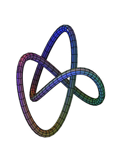
Figure 1: Tube plot of the trefoil knot curve, whose convex hull is exactly semidefinite representable with 3 liftings.

Using the standard change of variables

$$\cos\alpha=\frac{x_{0}^{2}-x_{1}^{2}}{x_{0}^{2}+x_{1}^{2}},\quad\sin\alpha=\frac{2x_{0}x_{1}}{x_{0}^{2}+x_{1}^{2}}$$

and trigonometric formulas, the space curve admits a rational representation as an affine projection of a sextic Veronese variety

$$\begin{array}[]{ll}{\mathcal{V}}=\{v\in{\mathbb{R}}^{3}\>:&1=(x_{0}^{2}+x_{1}^{2})^{3},\>v_{1}=(x_{0}^{2}+x_{1}^{2})(3x_{0}^{4}-12x_{0}^{2}x_{1}^{2}+x_{1}^{4}),\\ &v_{2}=2x_{0}x_{1}(x_{0}^{2}+x_{1}^{2})(5x_{0}^{2}-3x_{1}^{2}),\>v_{3}=4x_{0}x_{1}(x_{0}^{2}-3x_{1}^{2})(3x_{0}^{2}-x_{1}^{2}),\>\>x\in{\mathbb{R}}^{2}\}\end{array}$$

i.e. $n=3$, $m=1$ and $d=3$ in the notations of the previous section.

By Corollary 1, the convex hull of the trefoil knot curve is exactly semidefinite representable as

$$\mathrm{conv}\>{\mathcal{V}}=\{v\in{\mathbb{R}}^{3}\>:\>\left[\begin{array}[]{c}1\\ v\end{array}\right]=Ay,\>M_{3}(y)\succeq 0,\>y\in{\mathbb{R}}^{7}\}$$

with

$$A=\left[\begin{array}[]{rrrrrrr}1&0&3&0&3&0&1\\ 3&0&-9&0&-11&0&1\\ 0&10&0&4&0&-6&0\\ 0&12&0&-40&0&12&0\end{array}\right]$$

and

$$M_{3}(y)=\left[\begin{array}[]{cccc}y_{0}&*&*&*\\ y_{1}&y_{2}&*&*\\ y_{2}&y_{3}&y_{4}&*\\ y_{3}&y_{4}&y_{5}&y_{6}\end{array}\right]$$

where symmetric entries are denoted by stars. The affine system of equations involving $v$ and $y$ can be solved by Gaussian elimination to yield the equivalent formulation:

$$\begin{array}[]{l}\mathrm{conv}\>{\mathcal{V}}=\{v\in{\mathbb{R}}^{3}\>:\\ \quad\left[\begin{array}[]{cccc}\frac{1}{6}(3+v_{1}+2u_{1}-4u_{3})&*&*&*\\ \frac{1}{112}(10v_{2}+v_{3}+48u_{2})&\frac{1}{18}(3-v_{1}-20u_{1}-2u_{3})&*&*\\ \frac{1}{18}(3-v_{1}-20u_{1}-2u_{3})&\frac{1}{224}(6v_{2}-5v_{3}+96u_{2})&u_{1}&*\\ \frac{1}{224}(6v_{2}-5v_{3}+96u_{2})&u_{1}&u_{2}&u_{3}\end{array}\right]\succeq 0,\>\>u\in{\mathbb{R}}^{3}\}\end{array}$$

which is an explicit semidefinite representation with 3 liftings.

5.3 Steiner’s Roman surface

Quadratically parameterizable rational surfaces are classified in [3]. A well-known example is Steiner’s Roman surface, a non-orientable quartic surface with three double lines, which is parameterized as follows:

$${\mathcal{V}}=\{v\in{\mathbb{R}}^{3}\>:\>v_{1}=\frac{2x_{1}}{1+x_{1}^{2}+x_{2}^{2}},\>v_{2}=\frac{2x_{2}}{1+x_{1}^{2}+x_{2}^{2}},\>v_{3}=\frac{2x_{1}x_{2}}{1+x_{1}^{2}+x_{2}^{2}},\>\>x\in{\mathbb{R}}^{2}\}$$

see Figure 2.

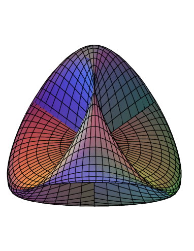
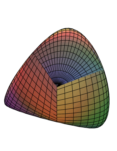
Figure 2: Two views of Steiner’s Roman surface, whose convex hull is semidefinite representable with 2 liftings.

The surface can be modeled as an affine projection of a quadratic Veronese variety:

$${\mathcal{V}}=\{v\in{\mathbb{R}}^{3}\>:\>1=x_{0}^{2}+x_{1}^{2}+x_{2}^{2},\>v_{1}=2x_{0}x_{1},\>v_{2}=2x_{0}x_{2},\>v_{3}=2x_{1}x_{2},\>\>x\in{\mathbb{R}}^{3}\}$$

i.e. $n=3$, $m=2$ and $d=1$ in the notations of the previous section. By Corollary 1, its convex hull is exactly semidefinite representable as

$$\mathrm{conv}\>{\mathcal{V}}=\{v\in{\mathbb{R}}^{3}\>:\>\left[\begin{array}[]{c}1\\ v\end{array}\right]=Ay,\>M_{1}(y)\succeq 0,\>y\in{\mathbb{R}}^{6}\}$$

with

$$A=\left[\begin{array}[]{rrrrrr}1&0&0&1&0&1\\ 0&2&0&0&0&0\\ 0&0&2&0&0&0\\ 0&0&0&0&2&0\end{array}\right]$$

and

$$M_{1}(y)=\left[\begin{array}[]{ccc}y_{00}&*&*\\ y_{10}&y_{20}&*\\ y_{01}&y_{11}&y_{02}\\ \end{array}\right].$$

The affine system of equations involving $v$ and $y$ can easily be solved to yield the equivalent formulation:

$$\mathrm{conv}\>{\mathcal{V}}=\{v\in{\mathbb{R}}^{3}\>:\>\left[\begin{array}[]{ccc}1-u_{1}-u_{2}&*&*\\ \frac{1}{2}v_{1}&u_{1}&*\\ \frac{1}{2}v_{2}&\frac{1}{2}v_{3}&u_{2}\end{array}\right]\succeq 0,\>\>u\in{\mathbb{R}}^{2}\}$$

which is an explicit semidefinite representation with 2 liftings.

5.4 Cayley cubic surface

Steiner’s Roman surface, studied in the previous paragraph, is dual to Cayley’s cubic surface $\{v\in{\mathbb{R}}^{3}\>:\>\det C(v)=0\}$ where

$$C(v)=\left[\begin{array}[]{ccc}1&*&*\\ v_{1}&1&*\\ v_{2}&v_{3}&1\end{array}\right].$$

The origin belongs to a set delimited by a convex connected component of this surface, admitting the following affine trigonometric parameterization:

$$\begin{array}[]{ll}{\mathcal{V}}=\{v\in{\mathbb{R}}^{3}\>:&v_{1}(\alpha)=\cos\alpha_{1},\>v_{2}(\alpha)=\sin\alpha_{2},\\ &v_{3}(\alpha)=\cos\alpha_{1}\sin\alpha_{2}-\cos\alpha_{2}\sin\alpha_{1},\>\alpha_{1}\in[0,\pi],\>\alpha_{2}\in[-\pi,\pi]\}.\end{array}$$

This is the boundary of the LMI region

$$\mathrm{conv}\>{\mathcal{V}}=\{v\in{\mathbb{R}}^{3}\>:\>C(v)\succeq 0\}$$

which is therefore semidefinite representable with no liftings. This set is a smoothened tetrahedron with four singular points, see Figure 3.

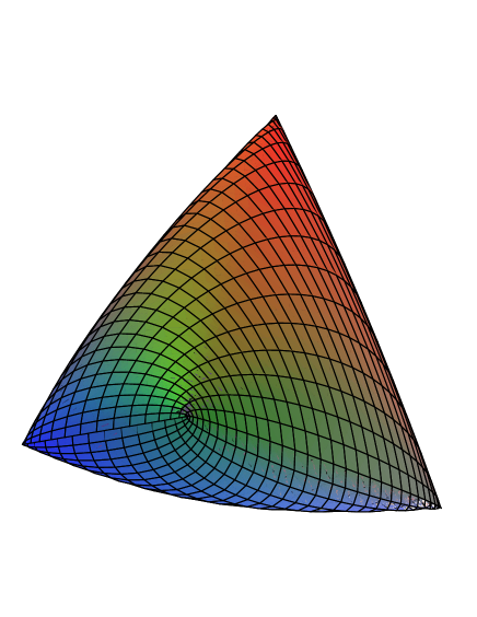
Figure 3: Convex connected component of Cayley’s cubic surface, semidefinite representable with no liftings.

Using the standard change of variables

$$\cos\alpha_{i}=\frac{x_{0}^{2}-x_{i}^{2}}{x_{0}^{2}+x_{i}^{2}},\quad\sin\alpha_{i}=\frac{2x_{0}x_{i}}{x_{0}^{2}+x_{i}^{2}},\quad i=1,2$$

we obtain an equivalent rational parameterization

$$\begin{array}[]{ll}{\mathcal{V}}=\{v\in{\mathbb{R}}^{3}\>:&1=(x_{0}^{2}+x_{1}^{2})(x_{0}^{2}+x_{2}^{2}),\>v_{1}=(x_{0}^{2}-x_{1}^{2})(x_{0}^{2}+x_{2}^{2}),\\ &v_{2}=2x_{0}x_{2}(x_{0}^{2}+x_{1}^{2}),\>v_{3}=2x_{0}(-x_{1}+x_{2})(x_{0}^{2}+x_{1}x_{2}),\>\>x\in{\mathbb{R}}^{3}\}.\end{array}$$

which is an affine projection of a quadratic Veronese variety, i.e. $n=3$, $m=2$ and $d=2$ in the notations of the previous section. By Corollary 1, its convex hull is exactly semidefinite representable as

$$\mathrm{conv}\>{\mathcal{V}}=\{v\in{\mathbb{R}}^{3}\>:\>\left[\begin{array}[]{c}1\\ v\end{array}\right]=Ay,\>M_{2}(y)\succeq 0,\>y\in{\mathbb{R}}^{15}\}$$

with $A$ of size $4$-by-$15$ and $M_{2}(y)$ of size $6$-by-$6$, not displayed here. It follows that $\mathrm{conv}\>{\mathcal{V}}$ is semidefinite representable as a $6$-by-$6$ LMI with $11$ liftings.

We have seen however that $\mathrm{conv}\>{\mathcal{V}}$ is also semidefinite representable as a $3$-by-$3$ LMI with no liftings, a considerable simplification. It would be interesting to design an algorithm simplifying a given semidefinite representation, lowering the size of the matrix and the number of variables. As far as we know, no such algorithm exists at this date.

6 Conclusion

The well-known equivalence between polynomial non-negativity and existence of a sum-of-squares decomposition was used, jointly with semidefinite programming duality, to identify the cases for which the convex hull of a rationally parameterized variety is exactly semidefinite representable. Practically speaking, this means that optimization of a linear function over such varieties is equivalent to semidefinite programming, at the price of introducing a certain number of lifting variables.

If the problem of detecting whether a plane algebraic curve is rationally parameterizable, and finding explicitly such a parametrization, is reasonably well understood from the theoretical and numerical point of view – see [12] and M. Van Hoeij’s algcurves Maple package for an implementation – the case of surfaces is much more difficult [13]. Up to our knowledge, there is currently no working computer implementation of a parametrization algorithm for surfaces. Since an explicit parametrization is required for an explicit semidefinite representation of the convex hull of varieties, the general case of algebraic varieties given in implicit form (i.e. as a polynomial equation), remains largely open.

Finally, we expect that these semidefinite representability results may have applications when studying non-convex semi-algebraic sets and varieties arising from stability conditions in systems control, in the spirit of [6, 7]. These developments are however out of the scope of the present paper.

References

- [1] A. Ben-Tal, A. Nemirovskii. Lectures on modern convex optimization. SIAM, 2001.
- [2] E. Brieskorn, H. Knörrer. Plane algebraic curves. Translated from the German by J. Stillwell. Birkäuser, 1986.
- [3] A. Coffman, A. J. Schwartz, C. Stanton. The algebra and geometry of Steiner and other quadratically parametrizable surfaces. Computer Aided Geometric Design 13:257-286, 1996.
- [4] L. Fialkow, J. Nie. Positivity of Riesz functional and solution of quadratic and quartic moment problems. J. Funct. Analysis 258:328-356, 2010.
- [5] J. W. Helton, J. Nie. Sufficient and necessary conditions for semidefinite representability of convex hulls and sets. SIAM J. Optim. 20(2):759-791, 2009.
- [6] D. Henrion, M. Šebek, V. Kučera. Positive polynomials and robust stabilization with fixed-order controllers. IEEE Trans. Autom. Control 48(7):1178-1186, 2003.
- [7] D. Henrion, J. B. Lasserre. Solving nonconvex optimization problems - How GloptiPoly is applied to problems in robust and nonlinear control. IEEE Control Syst. Mag. 24(3):72-83, 2004.
- [8] J. B. Lasserre. Convex sets with semidefinite representation. Math. Prog. 120:457–477, 2009.
- [9] M. Laurent. Sums of squares, moment matrices and optimization over polynomials. In: M. Putinar, S. Sullivant (Editors). Emerging applications of algebraic geometry. IMA Vol. Math. Appli. 149:157-270, Springer, 2009.
- [10] Y. Nesterov, A. Nemirovskii. Interior-point polynomial algorithms in nonlinear optimization. SIAM, 1994.
- [11] K. Ranestad, B. Sturmfels. On the convex hull of a space curve. arXiv:0912.2986, 2009.
- [12] J. R. Sendra, F. Winkler, S. Pérez-Díaz. Rational algebraic curves: a computer algebra approach. Springer, 2008.
- [13] J. Schicho. Rational parametrization of surfaces. J. Symbolic Comp. 26(1):1-29, 1998.