Bubble merging in breathing DNA as a vicious walker problem in opposite potentials

Abstract

We investigate the coalescence of two DNA-bubbles initially located at weak domains and separated by a more stable barrier region in a designed construct of double-stranded DNA. In a continuum Fokker-Planck approach, the characteristic time for bubble coalescence and the corresponding distribution are derived, as well as the distribution of coalescence positions along the barrier. Below the melting temperature, we find a Kramers-type barrier crossing behavior, while at high temperatures, the bubble corners perform drift-diffusion towards coalescence. In the calculations, we map the bubble dynamics on the problem of two vicious walkers in opposite potentials. We also present a discrete master equation approach to the bubble coalescence problem. Numerical evaluation and stochastic simulation of the master equation show excellent agreement with the results from the continuum approach. Given that the coalesced state is thermodynamically stabilized against a state where only one or a few base pairs of the barrier region are re-established, it appears likely that this type of setup could be useful for the quantitative investigation of thermodynamic DNA stability data as well as the rate constants involved in the unzipping and zipping dynamics of DNA, in single molecule fluorescence experiments.

I Introduction

Within a broad range of salt and temperature conditions, the Watson-Crick double-helix watson is the equilibrium structure of DNA. This thermodynamic stability is effected by hydrogen-bonding between paired bases and by base-stacking between nearest neighbor pairs of base pairs watson ; cantor ; kornberg ; kornberg1 ; frank ; delcourt ; krueger ; santalucia . By an increase of the temperature or by variation of the pH-value (titration with acid or alkali) double-stranded DNA progressively denatures, yielding regions of single-stranded DNA, until the double-strand is fully molten. This is the helix-coil transition poland ; peyrard_np . The melting temperature $T_{m}$ is defined as the temperature at which half of the DNA molecule has undergone denaturation poland ; frank ; guttmann ; wartell . Typically, the denaturation starts in regions rich in the weaker Adenine-Thymine base-pairs, and subsequently moves to zones of increasing Guanine-Cytosine content. The occurrence of zones of different stability within the genome was shown to be relevant when separating coding from non-coding regions carlon ; yeramian .

However, already at room temperature thermal fluctuations cause rare opening events of small intermittent denaturation zones in the double-helix gueron . These DNA bubbles consist of flexible single-stranded DNA, and their size fluctuates by step-wise zipping and unzipping of the base pairs (bps) at the zipper forks, where the bubble connects to the intact double-strand. Initiation of a bubble in a stretch of intact double-strand requires the crossing of a free energy barrier $\Delta G_{\rm bubble}$ of some 8 to 12 $k_{B}T$ at physiological temperature, corresponding to a Boltzmann factor, often referred to as the cooperativity factor, $\sigma_{0}=\exp(-\Delta G_{\rm bubble}/k_{B}T)\sim 10^{-5}\ldots 10^{-3}$. Once formed below the melting temperature $T_{m}$, a bubble will eventually zip close. Above $T_{m}$, a bubble will preferentially stay open and, if unconstrained, grow in size until it merges with other denaturation bubbles, eventually leading to full denaturation of the double-helix. Constraints against such full unzipping could, for instance, be the build-up of twist in smaller DNA-rings or the chemical connection of the two strands by short bulge-loops, compare Ref. altan .

Biologically, the physical conformations of DNA molecules are considered of increasing relevance for its function, see, for instance, the review ctn and references therein. In particular, the existence of intermittent (though infrequent) bubble domains is important, as the opening up of the Watson-Crick base pairs by breaking of the hydrogen bonds between complementary bases disrupts the helical stack. The flipping out of the ordered stack of the unpaired bases allows the binding of specific chemicals or proteins, that otherwise would not be able to access the reactive sites of the bases gueron ; poland ; krueger ; frank . In fact, there exists a competition of time scales between the opening/closing dynamics of DNA-bubbles and the binding kinetics of selectively single-stranded DNA binding proteins pant ; pant1 ; tobiasrc ; somepanwill . That the chemical potential of the single-stranded binding proteins does not lead to full denaturation of the DNA is due to the slow binding of the proteins when compared to the bubble dynamics pant ; pant1 ; tobiasrc ; somepanwill . It is also believed that DNA-breathing assists in the transcription initiation process tobiasprl ; tobiasbj ; choi ; kalosakas . The quantitative knowledge of the denaturation dynamics as well as energetics is imperative to a better understanding of genomic biochemical processes.

DNA-breathing has been modeled extensively in terms of the Peyrard-Bishop model, that is based on a set of Langevin equations for the base-base distance in a base pair; the effective attraction between the bases is represented by model potentials peyrard ; dauxois ; peyrard_cm ; campa ; peyrard_nonl . Alternatively, DNA-breathing can be considered as a random walk process in the free energy landscape of the Poland-Scheraga model of DNA denaturation, as the number of broken base pairs turns out to be the slow variable of the process altan . In continuum form, this approach to DNA bubble dynamics has been described in terms of a Fokker-Planck equation hame ; hans ; kafri . A discrete description, in which the coordinate of the random walker corresponds to a specific base pair, was suggested in Refs. bicout ; JPC ; tobiasrc ; tobiasprl , and the corresponding stochastic simulations analysis of DNA breathing was introduced in Ref. suman . The influence of a random energy landscape on bubble localization and dynamics was studied in Refs. hwa ; kafri ; jeon , while a framework to include an arbitrary given sequence of base pairs was developed in Refs. tobiasprl ; tobiasbj ; tobiaspre . Endowed with the sensitivity of their dynamics, DNA constructs were proposed as nanosensors tobiasjpc ; tobiasctn . We note that the formulation in terms of the gradient of the Poland-Scheraga free energy allows one to explicitly introduce all necessary independent stacking parameters based on the study krueger , see also the discussion in Ref. tobiasbj . Measuring the dynamics of DNA bubbles also provides information on the magnitude of the critical exponent $c$ representing the entropy loss factor of a closed polymer loop, deciding on the order of the denaturation transition poland1 ; fisher1 ; poland ; kafri1 ; comment ; haochme ; blossey , by influencing the temporal survival probability of bubbles hans ; kafri .

Figure 1: Schematic picture of the bubble coalescence setup in a designed DNA construct. It is clamped at both ends and consists of two outer soft zones (thin red lines) of lengths $N_{L},N_{R}$ bps with melting temperature $T_{s}$ and a stronger $N$-bps-long barrier zone (thick blue lines) with $T_{b}>T_{s}$. a) All bps closed ($T<T_{s}<T_{b}$). b) Soft zones open by raising the temperature above $T_{s}$. b₁–b₃) Successive opening of the barrier driven mainly by fluctuations ($T<T_{b}$) or drift ($T>T_{b}$) until coalescence. The discrete coordinates $X,Y=-N_{L},\dots,N+N_{R}$ are defined as the positions of the interfaces between the closed and broken bps.

The multi-state nature of DNA breathing can be monitored in real time on the single DNA level by fluorescence correlation techniques altan . It has been shown in a quantitative analysis that the experimentally accessible autocorrelation function is sensitive to the stacking parameters of DNA tobiasprl ; tobiasbj . However, it has not been fully appreciated to what extent the fluorophore and quencher molecules, that are attached to the DNA construct in the experiments reported in Refs. altan ; olegrev ; beacon , influence the stability of DNA. Moreover, the zipping rates measured in the single molecule fluorescence setup differ from those determined in NMR experiments gueron ; altan . We here propose and study a complementary setup for the single molecule fluorescence investigation of DNA breathing, as shown in Fig. 1. In this setup, a short stretch of DNA, clamped at both ends, is designed such that two soft zones consisting of weaker AT-bps are separated by a more stable barrier region rich in GC bps. For simplicity, we assume that both soft zones and barrier are homopolymers with a bp-dissociation free energy $\Delta G_{s}$ and $\Delta G_{b}$, respectively, and, in accordance with the experimental findings of reference altan , we neglect secondary structure formation in the barrier zone. At temperatures higher than the melting temperature $T_{s}$ of the soft zones, but still lower than the melting temperature $T_{b}$ of the barrier region such that two open bubbles are being promoted, thermal fluctuations will gradually dissociate the barrier, until the two bubbles coalesce. Note that the melting temperature at 100 mM salt conditions differs by approximately 50 degrees between mixed (AT/TA)_n and (GC/CG)_n homopolymers respectively santalucia ; krueger . This should provide a large enough temperature interval between hard and soft zones to perform this type of experiment. In the following we use realistic values for the simulations. Once coalesced, the free energy corresponding to one cooperativity factor $\sigma_{0}\sim 10^{-5}\ldots 10^{-3}$ is released, stabilizing the coalesced bubble against reclosure of the barrier. This fact should allow for a meaningful measurement of the coalescence time in experiment, and therefore provide a new and sensitive method to measure DNA stability data and base pair zipping rates. We also study the case when the system is prepared as above and then $T$ suddenly increased such that $T>T_{b}>T_{s}$ so that the system is driven towards coalescence. In both cases the two boundaries between bubbles and barrier perform a (biased) random walk in opposite free energy potentials.

In fact, the study of the bubble coalescence is of interest in its own right, as we map the random walk of the two zipper forks separating double-stranded barrier base-pairs from already denatured single-stranded bubble domains onto a new case of the vicious walker problem. Namely, we deal with two vicious walkers in linear but opposite potentials. The viciousness condition corresponds to the fact that when the two zipping forks meet, the bubbles coalesce, and the dynamics is stopped. While the problem of a general number of (otherwise noninteracting) vicious walkers in free space was solved long time ago fisher and has been only relatively recently generalized to the case of motion in a common potential bray , even two walkers in different potentials cannot be addressed analogously by the straightforward antisymmetrization procedure. To solve our problem in the continuum limit, we use a trick of introducing individual symmetry transformations for each walker which transform the respective Fokker-Planck operators to the same Hermitian form. In the transformed frame the problem is solved by the standard procedure constructing the joint probability density from the antisymmetrized product of the single-walker probability densities. This solution enables us to effectively reduce the numerical efforts needed for the evaluation of the joint probability density, mean coalescence time, spatial probability density of coalescence position, etc. by one dimension. Moreover, some of the quantities of interest can be obtained this way fully analytically including all the characteristics of the high-barrier case which are very hard to reliably determine numerically.

The paper is organized as follows. After introducing the discrete model in Sec. II and its continuum limit in Sec. III, we solve the latter in Sec. IV by using the symmetry of the problem. The main quantities of interest, namely, the coalescence time and its distribution, as well as the distribution of the coalescence position are obtained in Sec. V. In the following Sec. VI, we introduce a direct solution of the discrete problem via the complete master equation and a stochastic simulations scheme (Gillespie) and compare these results to those of the continuum approximation in Sec. VII. In Sec. VIII we address the connection between our models and results and real biologically relevant data. In the last Sec. IX we state our conclusions. Appendix A presents a detailed calculation of the auxiliary single-walker density. In Appendix B we explain the direct numerical solution to the full master equation of Sec. VI, while in Appendix C the Gillespie stochastic simulation scheme for the same master equation is briefly summarized.

II Defining the zipping and unzipping rates

In this section we define the transition rates for opening or closing a base pair, which are determined by two effects: the energy landscape stemming from the thermodynamical partition factors and the thermal fluctuations.

As illustrated in Fig. 1, we consider the case when the two soft bubble zones of the DNA construct are preferentially open, while the central barrier region is initially completely closed. We assume that the two soft zones are homopolymers with identical melting temperature $T_{s}$, and that the barrier region is a homopolymer with melting temperature $T_{b}>T_{s}$. In the following, we neglect secondary structure formation in the bubbles, consistent with experimental observations in relatively short bubble domains altan . The barrier region of initially closed base-pairs between the zipper forks will also be referred to as the clamp.

Each of the two DNA-bubbles is characterized by a partition factor of the form

$$\mathscr{Z}_{L}(X) = \frac{\sigma_{0}}{(X+N_{L}+1)^{c}}\prod_{\tilde{X}=-N_{L}}^{X}u(\tilde{X}),$$ (1)

$$\mathscr{Z}_{R}(Y) = \frac{\sigma_{0}}{(N+N_{R}-Y+1)^{c}}\prod_{\tilde{Y}=Y}^{N+N_{R}}u(\tilde{Y}),$$ (2)

where $X,Y\in[-N_{L},N+N_{R}]$ denote the positions of the left and right zipper fork, respectively. In Eqs. (1) and (2) the quantity $u(X)$, which takes the values $u_{s(b)}$, is the Boltzmann factor for breaking a base-pair in the soft zone (barrier domain), $u_{s(b)}=\exp\left(\beta\Delta G_{s(b)}\right)$, corresponding to the free energy $\Delta G_{s(b)}$ for breaking a base-pair; moreover, $\beta\equiv 1/[k_{B}T]$. We define $u(-N_{L})=u(N+N_{R})\equiv 1$.

Note once more the prefactor $(bubble\ length+1)^{-c}$ displaying the inherent long-range character of the Poland-Scheraga free energy model. It measures the reduction of the degrees of freedom of a loop configuration, as characterized by the critical exponent $c$ santalucia ; guttmann ; poland ; fisher1 ; fixman . For the long-time behavior in larger, single bubbles the influence of $c$ on the distribution of bubble lifetimes is considered in Refs. hans ; kafri in a continuum approach.

Finally, $\sigma_{0}$ is the cooperativity factor corresponding to the free energy barrier for breaking the first base-pair in a stretch of intact double-strand. Loosely speaking, it corresponds to the disruption of two stacking interactions in the DNA, while the single open base-pair’s entropy gain cannot balance the required enthalpy. This contrasts the opening of further base-pairs, for which the entropy gain almost balances the enthalpy cost. The cooperativity factor $\sigma_{0}$ helps stabilizing the coalesced DNA stretch against reclosure, as the combined free energy of the two individual bubbles carries a factor $\sigma_{0}^{2}$ while the coalesced bubble has only a factor $\sigma_{0}$.

The full partition function is

$$\mathscr{Z}(X,Y)=\mathscr{Z}_{L}(X)\mathscr{Z}_{R}(Y).$$ (3)

It defines the free energy landscape $\mathscr{F}(X,Y)=-\beta^{-1}\log\left[\mathscr{Z}(X,Y)\right]$, in which the random motion of the zipper forks takes place, as the gradient of $\mathscr{F}$ with respect to the coordinates $X$ and $Y$ defines the local driving forces experienced by the two zipper forks.

Below the melting temperature of the barrier $T_{b}$, the barrier will on average be driven towards closure, while above $T_{b}$ it will tend to denature completely. The effect of thermal fluctuations is to introduce a random walk-type dynamics of the position of the two zipper forks. Eventually, full denaturation of the clamp may be reached even below the melting temperature $T_{b}$. Once the two bubbles coalesce, the loop initiation (cooperativity) factor $\sigma_{0}$ is released, and the coalesced state becomes stabilized against closure.

Dynamically we quantify the random motion of the two zipper forks due to thermal fluctuations as follows. To zip close an already opened base-pair, we assume that this process is mainly governed by diffusion-limited encounter of the two separated bases, and subsequent bond formation. In contrast, to unzip a still closed base-pair, the free energy barrier embodied in the Boltzmann factor $u$ has to be overcome. For the left zipper fork we define $t^{+}_{L}(X,Y)$ which is the transfer coefficient for the process $X\rightarrow X+1$, corresponding to clamp size decrease, and $t^{-}_{L}(X,Y)$ the transfer coefficient for the process $X\rightarrow X-1$ (clamp size increase). For the right zipper fork we similarly introduce $t^{+}_{R}(X,Y)$ for the process $Y\rightarrow Y+1$ (clamp size increase) and $t^{-}_{R}(X,Y)$ for the process $Y\rightarrow Y-1$ (clamp size decrease). Due to the end clamping we require that $X\geq-N_{L}$ and $Y\leq N+N_{R}$, which amounts to introducing reflecting boundary conditions

$$t_{L}^{-}(X=-N_{L},Y)=0,$$ (4)

and

$$t_{R}^{+}(X,Y=N+N_{R})=0.$$ (5)

Once the clamp has vanished, we assume that the clamp will not be able to reform for a long time, and we impose the absorbing conditions

$$t_{L}^{-}(X,X)=t_{R}^{+}(Y,Y)=0.$$ (6)

Dynamically, this is connected to the time it takes the long stretch of single-strand to re-establish a base-pair in the clamp region (diffusion limit). In terms of the free energy the suppression of clamp reformation is due to the release of the free energy $\Delta G_{\rm bubble}$ corresponding to the cooperativity factor $\sigma_{0}$ on bubble coalescence (it would cost the additional factor $\sigma_{0}$ to reintroduce two single-strand/double-strand boundaries).

Knowledge of the transfer coefficients together with the boundary conditions above completely determine the dynamics, and we proceed by giving explicit expressions for the transfer coefficients in terms of the physical parameters of the problem. For the zipping rates we choose

$$t^{-}_{L}(X,Y)=\frac{1}{2}\mathcal{K}(X+N_{L}),$$ (7)

for the left fork, and identically for the right fork

$$t^{+}_{R}(X,Y)=\frac{1}{2}\mathcal{K}(N_{R}+N-Y).$$ (8)

We defined above a bubble-size-dependent rate coefficient

$$\mathcal{K}(q)=kq^{-\mu},$$ (9)

with $q$ being the number of broken bps in the bubble, where we have, as in previous studies, introduced the hook exponent $\mu$, related to the fact that during the zipping process not only the base-pair at the zipper fork is moved, but also part of the single-strand is dragged or pushed along. This additional effect may be included using similar arguments as in Refs. Di_Marzio_Guttman_Hoffman ; tobiasrc ; tobiasjpc : To zip close a base-pair, the two single-strands making up the bubble have to be pulled closer towards the zipper fork. The adjustment of pulling propagates along the contour of the chain until the closest bend (inflexion) is reached, a distance that scales as the gyration radius, i.e. $\simeq q^{\nu}$. Having in mind Rouse-type dynamics, this would slow down the unzipping rates by the factor $q^{-\nu}$. Hydrodynamic interactions may change the exponent and we here take the transfer coefficients above proportional to $q^{-\mu}$, with $\mu$ to be determined by more detailed microscopic investigations. The rate constant $k$ appearing in Eq. (9) is the rate constant for pure base pair unzipping without factors due to the coupling along the chain, i.e., the hook exponent. The factor $1/2$ introduced above in Eqs. (7), (8) is merely for convenience to be consistent with the nomenclature of previous approaches tobiasrc ; tobiasjpc . Apart from the hook effect, we thus assign a factor $k/2$ for the zipping at each of the forks.

As the DNA construct is embedded in a thermal bath, we require the zipping rates to fulfill the detailed balance conditions

$$t_{L}^{+}(X-1,Y)\mathscr{Z}(X-1,Y)=t_{L}^{-}(X)\mathscr{Z}(X,Y),$$ (10)

and

$$t_{R}^{-}(X,Y+1)\mathscr{Z}(X,Y+1)=t_{R}^{+}(X,Y)\mathscr{Z}(X,Y).$$ (11)

These conditions guarantee the relaxation to the thermodynamic equilibrium. For the left zipping rates this is fulfilled for

$$t_{L}^{+}(X,Y)=\frac{1}{2}\mathcal{K}(q_{L}+1)u(X+1)\{(q_{L}+1)/(q_{L}+2)\}^{c}.$$ (12)

Here $q_{L}=X+N_{L}$ is the length of the left bubble, and again $(bubble\ length+1)^{-c}$ is the correction for the entropy loss of a closed polymer loop, with $c$ being the loop exponent. For bubble size increase we thus take the transfer coefficients to be proportional to the Arrhenius-factor $u(X+1)$, multiplied by a loop correction factor. Note that for $q_{L}\rightarrow\infty$ the loop correction factor tends to $1$, which we will exploit later. For the right fork we similarly find

$$t_{R}^{-}(X,Y)=\frac{1}{2}\mathcal{K}(q_{R}+1)u(Y-1)\{(q_{R}+1)/(q_{R}+2)\}^{c},$$ (13)

where $q_{R}=N+N_{R}-Y$ is the length of the right bubble. We point out that Eqs. (7), (8), (12), and (13) are not unique in satisfying the detailed balance conditions, Eqs. (10) and (11). However, different choices correspond to redefinitions of the time unit $1/k$ which is the free parameter in our master equation approach and needs to be fixed from fit to experiment.

From the transition rates a master equation can be constructed for the conditional probability $P(X,Y;t|X_{0},Y_{0})$ with $X_{0},Y_{0}$ being the initial positions of the zipper forks. This master equation can be solved numerically, details of which are introduced in Sec. VI, and physical quantities such as the mean-first-passage time density can be calculated. However, based on four assumptions concerning the transition rates it is possible to derive a continuous Fokker-Planck equation approximating the full master equation description; this is done in Sec. III. From the Fokker-Planck approach we then derive numerical results for the coalescence time density, and both numerical and analytic expressions for the mean coalescence time and the probability density for the coalescence position in Secs. IV and V. These three following sections provide details and extensions of our previous short work twobubb .

III The Fokker-Planck approximation to the master equation

In this section we derive a Fokker-Planck approximation to the master equation based on the following assumptions:

• The temperature $T$ is so high compared to $T_{s}$ that the base pairs in the soft zones remain unzipped at all times, i.e. there are effectively reflecting boundary conditions at the interfaces between the soft zones and the barrier region;

• the soft zones are sufficiently long such that the influence of the loop factors can be neglected, and similarly

• the influence of the hook factors becomes sufficiently small.

• Finally, the number of bps in the barrier region is much bigger than one, i.e. $N\gg 1$, which allows for taking the continuum limit (see below).

Under the assumptions (i)–(iii) the full partition function for the two bubbles and the partially denatured barrier region becomes [see Eq. (3)]

$$\mathscr{Z}=\sigma_{0}^{2}u_{s}^{N_{L}+N_{R}}u_{b}^{X+N-Y},$$ (14)

where in this section $X,Y\in\{0,1,2,\dots,N\}$ due to (i) with $X\leq Y$. Notice that $X$ is the number of barrier base-pairs already broken from the left end of the barrier, and $N-Y$ counts the broken barrier base-pairs from the right end. The free energy is given as

$$\mathscr{F}=-2k_{B}T\log\sigma_{0}-(N_{L}+N_{R})\Delta G_{s}+(X+N-Y)\Delta G_{b}.$$ (15)

In the continuum limit (assumption (iv)) we introduce dimensionless coordinates $x=\tfrac{X}{N}$ and $y=\tfrac{Y}{N}$, $x,y\in[0,1]$. The gradient of $\mathscr{F}$ with respect to the coordinates $x$ and $y$ defines the local force experienced by the two zipper forks, namely

$$F_{X}=-\frac{d\mathscr{F}}{dx}=-N\Delta G_{b},\,\,F_{Y}=-\frac{d\mathscr{F}}{dy}=N\Delta G_{b}=-F_{X},$$ (16)

and we immediately see, that the zipper forks $X$ and $Y$ are driven by opposite, constant forces as sketched in Fig. 2.

Figure 2: Plot of the linear potentials experienced by the respective bubble interfaces in the case $T<T_{b}\ (f<0)$ in terms of the dimensionless quantities $x,y,f$ (see text for details).

Using the simplifications (ii) and (iii) stated above, the modified continuum rates (denoted by $r$ to distinguish them from the notation introduced in the discussion of the discrete case) for closing a base-pair at the left fork at position $x$, or at the right fork at position $y$, become [see Eqs. (7), (8), (12), and (13)]

$$r_{L}^{-}(x,y)=r_{R}^{+}(x,y)=k/2,$$ (17)

and

$$r_{L}^{+}(x,y)=r_{R}^{-}(x,y)=u_{b}k/2,$$ (18)

such that the zipping open of a base-pair requires crossing the barrier $\Delta G_{b}$. The boundary conditions

$$r_{L}^{-}(0,y)=r_{R}^{+}(x,1)=r_{L}^{+}(x,x)=r_{R}^{-}(y,y)=0,$$ (19)

guarantee that base-pairs cannot close beyond the barrier region, and that the process ends when the two zipper forks coalesce.

Define by $P(x,y;\tau)$ the probability distribution that the left and right zipper forks are located at $x$ and $y$, respectively, at some given time $\tau$. The time evolution of $P(x,y;\tau)$ is then given in terms of the master equation van_Kampen ; Risken

$$\frac{\partial}{\partial\tau}P(x,y;\tau) = r_{L}^{+}(x-1/N,y)P(x-1/N,y;\tau)+r_{L}^{-}(x+1/N,y)P(x+1/N,y;\tau)-\left[r_{L}^{-}(x,y)+r_{L}^{+}(x,y)\right]P(x,y;\tau)$$ (20)

$$+r_{R}^{-}(x,y+1/N)P(x,y+1/N;\tau)+r_{R}^{+}(x,y-1/N)P(x,y-1/N;\tau)-\left[r_{R}^{-}(x,y)+r_{R}^{+}(x,y)\right]P(x,y;\tau).$$

Following the standard derivation Gardiner ; van_Kampen we Taylor-expand the above master equation keeping the first two orders only. For instance, for the first term on the right hand side of Eq. (20), we obtain the Taylor expansion

$$r_{L}^{+}(x-1/N,y)P(x-1/N,y;\tau)\approx r_{L}^{+}(x,y)P(x,y;\tau)-\frac{1}{N}\frac{\partial}{\partial x}r_{L}^{+}(x,y)P(x,y;\tau)+\frac{1}{2N^{2}}\frac{\partial^{2}}{\partial x^{2}}r_{L}^{+}(x,y)P(x,y;\tau).$$ (21)

This is the only consistent expansion of finite order according to the Pawula-Marcinkiewicz theorem Risken ; pawula ; marcienkiewicz . Alternatively the full Kramers-Moyal expansion needs to be taken along. With analogous expansions for the other terms and after some rearrangement, we find the bivariate Fokker-Planck equation Risken

$$\frac{\partial}{\partial\tau}P(x,y;\tau|x_{0},y_{0})=F\left(\frac{\partial}{\partial y}-\frac{\partial}{\partial x}\right)P(x,y;\tau|x_{0},y_{0})+D\left(\frac{\partial^{2}}{\partial x^{2}}+\frac{\partial^{2}}{\partial y^{2}}\right)P(x,y;\tau|x_{0},y_{0}),$$ (22)

where, instead of the probability density $P(x,y;\tau)$, we use explicitly the notation $P(x,y;\tau|x_{0},y_{0})$ including the initial conditions $x_{0}$ and $y_{0}$. In Eq. (22), the force $F$ and diffusion constant $D$ are defined by

$$F\equiv\frac{k(u_{b}-1)}{2N},$$ (23)

and

$$D\equiv\frac{k(u_{b}+1)}{4N^{2}}.$$ (24)

Eq. (22) is completed by specifying the initial and boundary conditions. As initial condition, we choose the sharp $\delta$-form

$$P(x,y;0|x_{0},y_{0})=\delta(x-x_{0})\delta(y-y_{0}),$$ (25)

with $x_{0}<y_{0}$, and due to the initial condition Eq. (25) the joint probability density $P(x,y;\tau|x_{0},y_{0})$ is actually the Green’s function of Eq. (22). The condition that the two bubbles in the soft zones are always open is guaranteed by the reflecting boundary conditions (here, we define $2f\equiv F/D$)

$$\left.\left(\frac{\partial}{\partial x}-2f\right)P(x,y;\tau|x_{0},y_{0})\right|_{x=0}=0,$$

$$\left.\left(\frac{\partial}{\partial y}+2f\right)P(x,y;\tau|x_{0},y_{0})\right|_{y=1}=0,$$ (26)

at the edges of the line segment $[0,1]$: Once a zipper fork reaches either edge, the only possible direction to move is to restart unzipping the barrier. Moreover, we specify the viciousness condition

$$P(x,x;\tau|x_{0},y_{0})=0,$$ (27)

according to which the two zipper forks cannot be at the same point: the two forks annihilate and the bubbles coalesce. This last conditions ensures the continuous character of the probability density $P$. For completeness, we actually need to specify a second set of boundary conditions. However, due to the viciousness condition (27), we can choose this boundary condition ad libitum; a clever choice will turn out to be

$$\left.\frac{\partial}{\partial x}P(x,y;\tau|x_{0},y_{0})\right|_{x=1}=0,$$

$$\left.\frac{\partial}{\partial y}P(x,y;\tau|x_{0},y_{0})\right|_{y=0}=0.$$ (28)

Such a choice is possible because the zipper forks never reach these two points.

IV Solution of the vicious walker problem

IV.1 Transformation of the Fokker-Planck equation

To obtain the solution of the Fokker-Planck equation (22), it is convenient to notice that after a redefinition of time unit $t=D\tau$ the problem depends on a single dimensionless parameter

$$f=\frac{F}{2D}=N\frac{u_{b}-1}{u_{b}+1}.$$ (29)

It is important that this parameter depends on the length of the barrier $N$ and the Boltzmann factor $u_{b}$ for opening the barrier bps but not on the kinetic constant $k$. Thus, apart from an overall prefactor fixing the time unit, the solution depends solely on the structural properties of the physical system under study.

Let us summarize the rephrased problem in terms of $f$ for completeness

$$\left[-\frac{\partial}{\partial t}+\frac{\partial^{2}}{\partial x^{2}}+\frac{\partial^{2}}{\partial y^{2}}-2f\frac{\partial}{\partial x}+2f\frac{\partial}{\partial y}\right] P(x,y;t|x_{0},y_{0})=0,$$ (30a)

with boundary conditions

$$\left.\left(\frac{\partial}{\partial x}-2f\right)P(x,y;t|x_{0},y_{0})\right|_{x=0} =0,$$ (30b)

$$\left.\left(\frac{\partial}{\partial y}+2f\right)P(x,y;t|x_{0},y_{0})\right|_{y=1} =0,$$ (30c)

$$\left.\frac{\partial}{\partial x}P(x,y;t|x_{0},y_{0})\right|_{x=1} =0,$$ (30d)

$$\left.\frac{\partial}{\partial y}P(x,y;t|x_{0},y_{0})\right|_{y=0} =0,$$ (30e)

the viciousness condition

$$P(x,x;t|x_{0},y_{0})=0,$$ (30f)

and the ininitial condition

$$P(x,y;0|x_{0},y_{0})=\delta(x-x_{0})\delta(y-y_{0}) \text{ with }x_{0}<y_{0}.$$ (30g)

To proceed in the solution, let us first introduce the Fokker-Planck operators

$$\mathbb{L}_{\mathrm{FP}}^{+}(x)\equiv\frac{\partial^{2}}{\partial x^{2}}-2f\frac{\partial}{\partial x},$$ (31a)

$$\mathbb{L}_{\mathrm{FP}}^{-}(y)\equiv\frac{\partial^{2}}{\partial y^{2}}+2f\frac{\partial}{\partial y},$$ (31b)

so that the Fokker-Planck equation (30a) can be recast into the following form

$$\frac{\partial}{\partial t}P(x,y;t|x_{0},y_{0})=\Big{[}\mathbb{L}_{\mathrm{FP}}^{+}(x)+\mathbb{L}_{\mathrm{FP}}^{-}(y)\Big{]}P(x,y;t|x_{0},y_{0}).$$ (32)

The operators $\mathbb{L}_{\mathrm{FP}}^{+}(x)$ and $\mathbb{L}_{\mathrm{FP}}^{-}(y)$ can now be used to transform our Fokker-Planck equation following the procedure outlined in Ref. Risken , Chapter 5.4. Let us now define the Hermitian operator

$$\mathbb{L}(x,x_{0})\equiv e^{-f(x-x_{0})}\mathbb{L}_{\mathrm{FP}}^{+}(x)e^{f(x-x_{0})}=\frac{\partial^{2}}{\partial x^{2}}-f^{2}.$$ (33)

Here the last equality sign can be shown by applying the operator to a test function. The operator $\mathbb{L}(x,x_{0})$ corresponds to a Hamilton operator of a Schrödinger equation with imaginary time $-i\hbar t$, mass $m=\hbar^{2}/2$ and a constant potential $f^{2}$. The idea is that it is (in general) easier to solve the time-dependent Schrödinger equation than the Fokker-Planck equation, because the first-order derivative has been eliminated. The relation between the solutions of the original and the transformed Fokker-Planck equations are found after a few lines of algebra, and we obtain the following result: If $\widetilde{p}^{L}(x;t|x_{0})$ is a solution of

$$\frac{\partial}{\partial t}\widetilde{p}^{L}(x;t|x_{0})=\mathbb{L}(x,x_{0})\widetilde{p}^{L}(x;t|x_{0}),$$ (34)

then the density

$$p^{L}(x;t|x_{0})=\exp[f(x-x_{0})]\widetilde{p}^{L}(x;t|x_{0})$$ (35)

solves the original equation

$$\frac{\partial}{\partial t}p^{L}(x;t|x_{0})=\mathbb{L}_{\mathrm{FP}}^{+}(x)p^{L}(x;t|x_{0}).$$ (36)

The boundary conditions in $x$, Eqs. (30b) and (30d), are transformed to

$$\left.\left(\frac{\partial}{\partial x}-f\right)\widetilde{p}^{L}(x;t|x_{0})\right|_{x=0}=0,$$ (37a)

$$\left.\left(\frac{\partial}{\partial x}+f\right)\widetilde{p}^{L}(x;t|x_{0})\right|_{x=1}=0,$$ (37b)

while the initial condition remains unchanged, $\widetilde{p}^{L}(x;t=0|x_{0})=\exp[-f(x-x_{0})]p^{L}(x;t=0|x_{0})=\delta(x-x_{0})$. In other words, with Eqs. (33), (37a), and (37b) we have indeed transformed the original Fokker-Planck operator $\mathbb{L}_{\mathrm{FP}}^{+}(x)$ into Hermitian form.

Noticing that

$$\mathbb{L}(y,y_{0})=\frac{\partial^{2}}{\partial y^{2}}-f^{2}=e^{f(y-y_{0})}\mathbb{L}_{\mathrm{FP}}^{-}(y)e^{-f(y-y_{0})},$$ (38)

the same procedure can be carried out for the $y$-coordinate, where the different sign in front of $f$ in Eq. (30a) causes that, if $\widetilde{p}^{R}(y;t|y_{0})$ is a solution to

$$\frac{\partial}{\partial t}\widetilde{p}^{R}(y;t|y_{0})=\mathbb{L}(y,y_{0})\widetilde{p}^{R}(y;t|y_{0}),$$ (39)

then

$$p^{R}(y;t|y_{0})=\exp\left[-f(y-y_{0})\right]\widetilde{p}^{R}(y;t|y_{0})$$ (40)

satisfies

$$\frac{\partial}{\partial t}p^{R}(y;t|y_{0})=\mathbb{L}_{\mathrm{FP}}^{-}(y)p^{R}(y;t|y_{0}),$$ (41)

and the boundary conditions are

$$\left.\left(\frac{\partial}{\partial y}+f\right)\widetilde{p}^{R}(y;t|y_{0})\right|_{y=1}=0,$$ (42a)

$$\left.\left(\frac{\partial}{\partial y}-f\right)\widetilde{p}^{R}(y;t|y_{0})\right|_{y=0}=0,$$ (42b)

together with $\tilde{p}^{R}(y;t=0|y_{0})=\delta(y-y_{0})$.

We now see why Eqs. (30d), (30e) are clever choices for the additional boundary conditions on $P(x,y;t|x_{0},y_{0})$, together with the similarity transformations (35) and (40): reflecting the uneven symmetry of the problem with respect to the original coordinates, all equations defining the functions $\widetilde{p}^{L}(x;t|x_{0})$ and $\widetilde{p}^{R}(x;t|x_{0})$ are identical, and thus are the functions themselves

$$\tilde{p}^{L}(x;t|x_{0})=\tilde{p}^{R}(x;t|x_{0})=\tilde{p}(x;t|x_{0}).$$ (43)

IV.2 Solution of the transformed Fokker-Planck equation

After the individual similarity transformations for the left (35) and right (40) walker, respectively, are performed, we arrive at the following time-dependent Schrödinger equation

$$\frac{\partial}{\partial t}\widetilde{P}(x,y;t|x_{0},y_{0})=\left[\mathbb{L}(x,x_{0})+\mathbb{L}(y,y_{0})\right]\widetilde{P}(x,y;t|x_{0},y_{0}),$$ (44)

with imaginary time; here,

$$\widetilde{P}(x,y;t|x_{0},y_{0})=e^{-f(x-x_{0})+f(y-y_{0})}P(x,y;t|x_{0},y_{0}),$$ (45)

which implies the same viciousness condition $\widetilde{P}(x,x;t|x_{0},y_{0})=0$ as in the original formulation. Now, however, we effectively have two identical vicious walkers moving in a common (constant) potential for which the solution is well known fisher ; bray . It is given by the antisymmetric product of the single-walker solutions, namely

$$\widetilde{P}(x,y;t|x_{0},y_{0})=\tilde{p}(x;t|x_{0})\tilde{p}(y;t|y_{0})-\tilde{p}(y;t|x_{0})\tilde{p}(x;t|y_{0}).$$ (46)

Note that this form of the solution is analogous to constructing the solution of an absorbing boundary value problem for a single diffusor under a constant drift according to the method of images redner .

The backward transformation of the solution (46) by inverting Eq. (45) finally produces

$$P(x,y;t|x_{0},y_{0})=e^{f(x-x_{0})-f(y-y_{0})}\left[\tilde{p}(x;t|x_{0})\tilde{p}(y;t|y_{0})-\tilde{p}(y;t|x_{0})\tilde{p}(x;t|y_{0})\right],$$ (47)

and by construction this is a solution of Eq. (30a), satisfying the boundary conditions Eqs. (30b)–(30e), as well as the viciousness condition $P(x,x;t|x_{0},y_{0})=0$. It remains to check that this solution also satisfies the initial condition (30g) and, thus, fully solves the studied problem. For $t=0$ we obtain

$$P(x,y;t=0|x_{0},y_{0}) = e^{f(x-x_{0})-f(y-y_{0})}\left[\delta(x-x_{0})\delta(y-y_{0})-\delta(y-x_{0})\delta(x-y_{0})\right]$$ (48)

$$= \delta(x-x_{0})\delta(y-y_{0})-e^{2f(y_{0}-x_{0})}\delta(y-x_{0})\delta(x-y_{0})$$

$$= \delta(x-x_{0})\delta(y-y_{0}),$$

valid for $x_{0}<y_{0}$ and $x<y$. The last equality follows because of the choice of the initial condition $x_{0}<y_{0}$ and the viciousness of the process, i.e. the walkers can never pass each other, which also implies $x<y$ for any realizable configuration at any time $t$. Thus, the arguments of the $\delta$-functions in the second term can never vanish simultaneously and therefore this term is effectively equal to zero. Thus (47) is the solution to our problem.

IV.3 Calculation of $\tilde{p}(x;t|x_{0})$ and its spectral resolution

To find the solution of the full 2-walker problem (47) we need to calculate $\widetilde{p}(x;t|x_{0})$, which solves the Schrödinger equation

$$\frac{\partial}{\partial t}\widetilde{p}(x;t|x_{0})=\left[\frac{\partial^{2}}{\partial x^{2}}-f^{2}\right]\widetilde{p}(x;t|x_{0}),$$ (49)

and satisfies the boundary conditions Eqs. (37a) and (37b), as well as the initial condition $\widetilde{p}(x;t=0|x_{0})=\delta(x-x_{0})$. Unfortunately, there is no explicit solution of this equation in the time domain. It can be found, however, in the Laplace picture which is done in detail in Appendix A. Here we only summarize the final result

$$\tilde{p}(x;z|x_{0}) = \frac{1}{2k(\kappa^{2}e^{2k}-1)}\left[e^{k|x-x_{0}|}+\kappa^{2}e^{2k}e^{-k|x-x_{0}|}\right.$$ (50)

$$\left.+\kappa e^{(x+x_{0})k}+\kappa e^{2k}e^{-(x+x_{0})k}\right],$$

with $z$-dependent

$$k\equiv k(z)=\sqrt{z+f^{2}},$$ (51)

and

$$\kappa\equiv\kappa(z)=\frac{k(z)+f}{k(z)-f}.$$ (52)

The corresponding behavior in the time domain is found by the inverse Laplace transform

$$\tilde{p}(x;t|x_{0}) = \int_{\epsilon-i\infty}^{\epsilon+i\infty}\frac{dz}{2\pi i}e^{zt}\tilde{p}(x;z|x_{0})$$ (53)

$$= \sum_{n=0}^{\infty}e^{\lambda_{n}t}\psi_{n}(x)\psi^{*}_{n}(x_{0})$$

with $\epsilon\geq 0$ large enough such that all singularities of $\tilde{p}(x;z|x_{0})$ lie in the half-plane $\mathrm{Re}\,z<\epsilon$. We used the formal eigenmode expansion in the second line of the above equation which exists as a spectral resolution of the Hermitian operator defined by Eq. (49) and the pertinent boundary conditions (37a) and (37b). The eigenvalues $\lambda_{n}$ are real numbers since the operator is Hermitian, but not necessarily non-positive like in the case of standard Fokker-Planck operators in one dimension. The reason is that $\tilde{p}(x;t|x_{0})$ is an auxiliary mathematical quantity without any direct physical meaning and, thus, can in principle grow exponentially over time, i.e., some of the $\lambda_{n}$ might be positive. The physical quantity which is not allowed to grow indefinitely is the 2-walker Green’s function (47). This is useful to keep in mind when studying the spectral resolutions of (50) and (47) in more detail in the following.

The spectrum of the operator $\partial^{2}/\partial x^{2}-f^{2}$ from Eq. (49), together with the boundary conditions, can be found either directly from the defining equations or by finding the poles of the 1-walker Green’s function (50). Indeed, the secular equation obtained by either method is equivalent to the denominator in Eq. (50) being zero, i.e., $\kappa^{2}(\lambda)=e^{-2k(\lambda)}$. This leads to transcendent equations for real $\lambda$ in the respective ranges

$$(\lambda+2f^{2})\sinh\sqrt{\lambda+f^{2}}+2f\sqrt{\lambda+f^{2}}\cosh\sqrt{\lambda+f^{2}} =0\quad\text{for }\lambda\geq-f^{2}$$ (54a)

$$(\lambda+2f^{2})\sin\sqrt{|\lambda|-f^{2}}+2f\sqrt{|\lambda|-f^{2}}\cos\sqrt{|\lambda|-f^{2}} =0\quad\text{for }\lambda\leq-f^{2}\ .$$ (54b)

One looks for solutions of these equations in their ranges of validity. Thus, with the help of the standard graphical analysis, it turns out that the first equation (54a) has at least one solution only for $f<0$, this solution is positive, i.e. $\lambda_{0}>0$. When $f<-2$ a further solution with $-f^{2}<\lambda_{1}<0$ solves Eq. (54a). There are no more options for Eq. (54a). On the other hand, the second equation (54b) always has an infinite number of solutions. For $f>0$ these solutions are bounded by $-f^{2}-(n+1)^{2}\pi^{2}\leq\lambda_{n}\leq-f^{2}-n^{2}\pi^{2}$ ($n=0,1,2,\dots$). For $0>f>-2$ the first eigenvalue $\lambda_{0}$ satisfies Eq. (54a) while the remaining eigenvalues ($\lambda_{n}$ for $n=1,2,\dots$) stem from Eq. (54b) and are still bounded by $-f^{2}-n^{2}\pi^{2}\leq\lambda_{n}\leq-f^{2}-(n-1)^{2}\pi^{2}$. Finally, for $f<-2$ the first two eigenvalues $\lambda_{0}$ and $\lambda_{1}$ are determined by Eq. (54a) and the rest stems from Eq. (54b) being bounded by $-f^{2}-n^{2}\pi^{2}\leq\lambda_{n}\leq-f^{2}-(n-1)^{2}\pi^{2}$ for $n=2,3,\dots$.

There are two special values of the force $f=0,-2$ where the spectrum appears to change its analytic structure. First, the $f=0$ case corresponds to the problem of two vicious walkers freely diffusing in an impenetrable well, i.e. in a common potential. For this case, we do not need to use our trick as it is solved already by a previous study bray : The single-walker spectrum reads $\lambda_{n}=(n\pi)^{2}$ for $n=0,1,2,\dots$ The second case, $f=-2$, does not appear to be in any way particular physically. Actually, neither of the two cases have any exceptional physical properties — all the physical quantities change smoothly across these two points when changing $f$. The apparent singularities occur only in the auxiliary quantities. Technically, these two cases are the only ones where the trivial solution $\lambda=-f^{2}$ of Eqs. (54) corresponds to a non-trivial, i.e. non-zero, solution for the eigenfunction. Mathematically, this is reflected by the formal failure when $k(z)=0$ of the method used in Appendix A leading to Eq. (50). In such cases, the two fundamental solutions $e^{\pm kx}$ of Eq. (98) become identical and equal to a constant. The second independent solution is then linear in $x$ according to the elementary theory of linear differential equations. Thus, the two special cases are not directly covered by the general solution presented in App. A and all formulas stemming from it. We do not give explicit solutions for those two singular cases since all quantities of interest can be obtained from the general formulas by taking the appropriate limit $f\to 0$, or $-2$.

Now, if we insert the expansion (53) into Eq. (47) we see that the spectrum of that equation is given by all pairwise sums of different 1-walker eigenvalues, i.e. $\Lambda_{k}=\lambda_{i}+\lambda_{j}\ (i\neq j)$ [the sums of identical 1-walker eigenvalues have zero weight due to the anti-symmetrization in (47)]. Therefore, the first two 1-walker solutions $\lambda_{0}$ and $\lambda_{1}$ determine the long-time asymptotics of the 2-walker problem. For large negative $f\ll-1$, corresponding to a large barrier case, the asymptotic behavior is dominating the whole solution and, thus, the combination $\Lambda_{0}\equiv\lambda_{0}+\lambda_{1}$ effectively determines the interesting quantities such as the mean coalescence time or the probability distribution of the coalescence position. This allows us to get full analytic results in the limit $f\ll-1$, as explicitly derived in Section V.2. In this case both eigenvalues $\lambda_{0,1}$ are solutions of Eq. (54a), and they are exponentially small in $|f|$. They can be found to leading order from the second order expansion in $\lambda$ of Eq. (54a), yielding $\lambda_{0,1}\simeq\pm 4f^{2}e^{-|f|}$. To obtain $\Lambda_{0}$ we need to increase the accuracy by expanding the equation up to the third order in $\lambda$ and we find $\Lambda_{0}=\lambda_{0}+\lambda_{1}\simeq-16f^{2}(|f|-1)e^{-2|f|}$ which is negative, as it should be since $P(x,y;t|x_{0},y_{0})$ cannot grow exponentially, $P$ being a physical quantity. So, despite the existence of a positive 1-walker eigenvalue $\lambda_{0}$, the physically relevant combination $\lambda_{0}+\lambda_{1}<0$ ensures meaningful results.

V Bubble coalescence time and position from the solution of the Fokker-Planck equation

V.1 General treatment

From the solution of the Fokker-Planck equation, we now calculate in general the quantities of interest, namely the characteristic coalescence time of the two random walking zipper forks, and the probability distribution of the coalescence position. In the time domain this is done by considering the conservation of probability in the form

$$\Pi(t|x_{0},y_{0})+\int_{0}^{1}dy\int_{0}^{y}dxP(x,y;t|x_{0},y_{0})=1,$$ (55)

which is actually a defining equation for the probability $\Pi(t|x_{0},y_{0})$ that the walkers have met before time $t$. Consequently, the second term represents the probability of having two separate bubbles at time $t$ (survival probability). Note the range of integration restricting $x\in[0,y)$. The probability density associated with $\Pi(t|x_{0},y_{0})$ is

$$\begin{split}\pi(t|x_{0},y_{0})&\equiv\frac{d}{dt}\Pi(t|x_{0},y_{0})\\ &=-\int_{0}^{1}dy\int_{0}^{y}dx\frac{\partial}{\partial t}P(x,y;t|x_{0},y_{0}),\end{split}$$ (56)

which, after invoking Eq. (30a) and rearranging the order of the integrals, yields

$$\begin{split}\pi(t|x_{0},y_{0})&=-\int_{0}^{1}dy\int_{0}^{y}dx\left[\frac{\partial^{2}}{\partial x^{2}}-2f\frac{\partial}{\partial x}\right]P(x,y;t|x_{0},y_{0})-\int_{0}^{1}dx\int_{x}^{1}dy\left[\frac{\partial^{2}}{\partial y^{2}}+2f\frac{\partial}{\partial y}\right]P(x,y;t|x_{0},y_{0})\\ &=-\int_{0}^{1}dy\left[\left\{\frac{\partial}{\partial x}-2f\right\}P(x,y;t|x_{0},y_{0})\right]_{0}^{y}-\int_{0}^{1}dx\left[\left\{\frac{\partial}{\partial y}+2f\right\}P(x,y;t|x_{0},y_{0})\right]_{x}^{1}\\ &=-\int_{0}^{1}dy\left\{\frac{\partial}{\partial x}-2f\right\}P(x,y;t|x_{0},y_{0})\Bigg{|}_{x=y}+\int_{0}^{1}dx\left\{\frac{\partial}{\partial y}+2f\right\}P(x,y;t|x_{0},y_{0})\Bigg{|}_{y=x}\\ &=\int_{0}^{1}dx\left\{\frac{\partial}{\partial y}-\frac{\partial}{\partial x}+4f\right\}P(x,y;t|x_{0},y_{0})\Bigg{|}_{y=x}=\int_{0}^{1}dx\left\{\frac{\partial}{\partial y}-\frac{\partial}{\partial x}\right\}P(x,y;t|x_{0},y_{0})\Bigg{|}_{y=x},\end{split}$$ (57)

where the boundary conditions imposed on $P(x,y;t|x_{0},y_{0})$ and the viciousness condition have been used in subsequent manipulations. The quantity $\pi(t|x_{0},y_{0})$ can be interpreted as the probability current flowing into the absorbing boundary, here given by the line $x=y$ (compare with an analogous discussion for a 1-dimensional case in Ref. Novotny2000 ).

From the last relation, we define the quantity $\varrho(x;t|x_{0},y_{0})$, the coalescence-position-resolved probability density for the coalescence time,

$$\pi(t|x_{0},y_{0})=\int_{0}^{1}dx\,\varrho(x;t|x_{0},y_{0}),$$ (58)

such that

$$\varrho(x;t|x_{0},y_{0})=\left\{\frac{\partial}{\partial y}-\frac{\partial}{\partial x}\right\}P(x,y;t|x_{0},y_{0})\Bigg{|}_{y=x}.$$ (59)

We are mainly interested in either the mean coalescence time $\tau(x_{0},y_{0})=\int_{0}^{\infty}dt\,t\,\pi(t|x_{0},y_{0})$ or the probability density of the coalescence position $\rho(x|x_{0},y_{0})=\int_{0}^{\infty}dt\,\varrho(x;t|x_{0},y_{0})$. These are quantities integrated over time and, thus, they may be determined from the solution in the Laplace domain without explicit knowledge of $P(x,y;t|x_{0},y_{0})$ in the time domain.

We now rewrite Eq. (47) in terms of the inverse Laplace transforms as follows

$$P(x,y;t|x_{0},y_{0})=\int_{\epsilon-i\infty}^{\epsilon+i\infty}\frac{dz_{1}}{2\pi i}e^{z_{1}t}\int_{\epsilon-i\infty}^{\epsilon+i\infty}\frac{dz_{2}}{2\pi i}e^{z_{2}t}e^{f(x-y-x_{0}+y_{0})}[\tilde{p}(x;z_{1}|x_{0})\tilde{p}(y;z_{2}|y_{0})-\tilde{p}(y;z_{1}|x_{0})\tilde{p}(x;z_{2}|y_{0})],$$ (60)

where $\tilde{p}(x;z|x_{0})$ is given in (50). In case that $\tilde{p}(x;z|x_{0})$ has no poles in the half-plane ${\rm Re}z>0$ (corresponding to $f>0,\,\epsilon=0$), we can directly use the substitution $z_{1}=z/2+i\omega$, $z_{2}=z/2-i\omega$; $z=z_{1}+z_{2}$, and $\omega=(z_{1}-z_{2})/(2i)$, to obtain a single inverse Laplace transform for $P(x,y;t|x_{0},y_{0})$, namely

$$P(x,y;t|x_{0},y_{0})=\int_{-i\infty}^{i\infty}\frac{dz}{2\pi i}e^{zt}\int_{-\infty}^{\infty}\frac{d\omega}{2\pi}e^{f(x-y-x_{0}+y_{0})} \left[\tilde{p}\left(x;z/2+i\omega|x_{0}\right)\tilde{p}\left(y;z/2-i\omega|y_{0}\right)\right.$$ (61)

$$\left.-\tilde{p}\left(y;z/2+i\omega|x_{0}\right)\tilde{p}\left(x;z/2-i\omega|y_{0}\right)\right].$$

Thus, we can identify the Laplace transform $\tilde{P}(x,y;z|x_{0},y_{0})$ of $P(x,y;t|x_{0},y_{0})$ for $f>0$ as

$$\tilde{P}(x,y;z|x_{0},y_{0})=\int_{-\infty}^{\infty}\frac{d\omega}{2\pi}e^{f(x-y-x_{0}+y_{0})}[\tilde{p}(x;z/2+i\omega|x_{0})\tilde{p}(y;z/2-i\omega|y_{0})-\tilde{p}(y;z/2+i\omega|x_{0})\tilde{p}(x;z/2-i\omega|y_{0})].$$ (62)

This directly yields, by means of relations (58) and (59), the Laplace transforms $\tilde{\pi}(z|x_{0},y_{0})$ and $\tilde{\varrho}(x;z|x_{0},y_{0})$, from which we in turn deduce the (time-averaged) distribution of coalescence positions,

$$\rho(x|x_{0},y_{0})=\tilde{\varrho}(x;z=0^{+}|x_{0},y_{0}),$$ (63)

and the characteristic (mean) coalescence time

$$\tau(x_{0},y_{0})=-\left.\frac{d}{dz}\tilde{\pi}(z|x_{0},y_{0})\right|_{z=0^{+}}.$$ (64)

For $f<0$ the situation is more complicated since $\tilde{p}(x;z|x_{0})$ in this case has a pole at $\lambda_{0}>0$ which prohibits us from just repeating the above reasoning. The Laplace transform (60) only holds for ${\rm Re}\,z_{1,2}>\lambda_{0}>0$ implying ${\rm Re}\,z>2\lambda_{0}>0$ and the analytic continuation down to $z=0$ is not obvious. However, since we know the position of the only pole located in the ${\rm Re}\,z>0$ half-plane, we can treat this singularity separately and thus generalize the previous results. Using the Cauchy theorem for complex integrals we move the integration line from $\epsilon+i\omega$ with $\epsilon>\lambda_{0}>0$ down to the imaginary axis and add the contribution from the (single) singularity at $\lambda_{0}$ in between these two lines. This method eventually leads to an expression for the Laplace transform $P(x,y;z|x_{0},y_{0})$ in the whole half-plane $\mathrm{Re}\,z>0$ for $f<0$,

$$\begin{split}\tilde{P}(x,y;z|x_{0},y_{0})&=e^{f(x-y-x_{0}+y_{0})}\bigg{\{}\int_{-\infty}^{\infty}\frac{d\omega}{2\pi}[\tilde{p}(x;z/2+i\omega|x_{0})\tilde{p}(y;z/2-i\omega|y_{0})-\tilde{p}(y;z/2+i\omega|x_{0})\tilde{p}(x;z/2-i\omega|y_{0})]\\ &+{\rm Res}_{z_{1}=\lambda_{0}}\tilde{p}(x;z_{1}|x_{0})\tilde{p}(y;z-\lambda_{0}|y_{0})-{\rm Res}_{z_{1}=\lambda_{0}}\tilde{p}(y;z_{1}|x_{0})\tilde{p}(x;z-\lambda_{0}|y_{0})\\ &+\tilde{p}(x;z-\lambda_{0}|x_{0}){\rm Res}_{z_{2}=\lambda_{0}}\tilde{p}(y;z_{2}|y_{0})-\tilde{p}(y;z-\lambda_{0}|x_{0}){\rm Res}_{z_{2}=\lambda_{0}}\tilde{p}(x;z_{2}|y_{0})\bigg{\}},\end{split}$$ (65)

which is the sought-for generalization of (62). We observe that the double-residue term drops out due to the antisymmetrization procedure.

V.2 Results

Eqs. (62) and (65) for $f>0$ and $f<0$, respectively, together with the single-walker Green’s function (50) and the identities for $\rho(x|x_{0},y_{0})$ (63) and $\tau(x_{0},y_{0})$ (64) were implemented in MATHEMATICA and evaluated. The results are shown in Figs. 3 and 4 depicting the coalescence position probability density for several values of $f$ and the mean coalescence time as a function of $f$, respectively. Both quantities are shown for two different initial conditions $x_{0}=0,\,y_{0}=1$ (the two walkers start out right at the boundaries) and $x_{0}=0.5,\,y_{0}=0.9$ (a generic initial condition). Further results for the coalescence time probability density $\pi(t|x_{0},y_{0})$ (57) are presented in later sections.

The results for the coalescence position in Fig. 3 show for both initial conditions a clear crossover from a peaked form of the probability density for large positive force (the case of an almost “free fall” into the potential well where the boundary conditions have negligible influence on the dynamics, studied in detail in Ref. hame and discussed below) to a very flat probability density in the case of large negative force corresponding to a high barrier. The flatness in the latter case can be understood from a simple Arrhenius-like model, in which the probability of the walker to be at a place $x$ is proportional to a Boltzmann weight, i.e., $\exp[-\beta\phi(x)]$, where $\phi(x)=-\int^{x}F(x^{\prime})dx^{\prime}$ is the free energy corresponding to the force $F(x)=\pm f$. Since we are now dealing with two walkers, the probability of both of them being simultaneously at the coalescence position is given by the product of the Boltzmann weights, $\exp(-\beta[\phi_{L}(x)+\phi_{R}(x)])$, which is a position-independent constant due to the cancelation of the position-dependence of the two opposite linear potentials. This simple picture breaks down close to the boundaries but otherwise is sufficient to grasp the observed behavior.

The characteristic (mean) coalescence times in Fig. 4 cross over from the “free fall” behavior for $f\gg 1$, proportional to the inverse of the force $\tau\simeq 1/f$ (using the natural boundary condition in the calculation of Ref. hame gives $\tau=(y_{0}-x_{0})/(4f)$, cf. Eq. (9) therein) to the thermal Arrhenius/Kramers-like barrier crossing proportional to the exponential of the barrier height $\tau\simeq\exp(2|f|)$ for $f\ll-1$. Thus, all the results are plausible and can be qualitatively rationalized based on simple physical arguments.

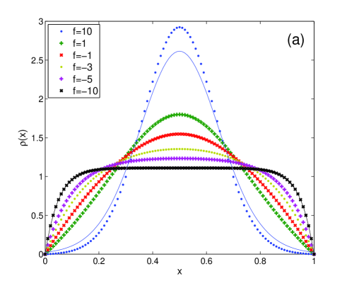
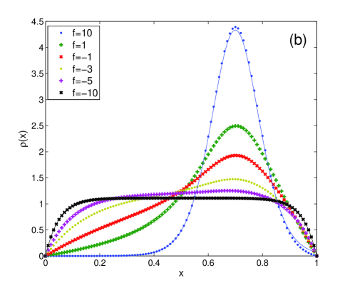
Figure 3: Probability density for the coalescence position $\rho(x|x_{0},y_{0})$ as a function of the position $x$ for several values of the dimensionless force $f$. The initial positions of the walkers $x_{0}$ and $y_{0}$ were $x_{0}=0,\,y_{0}=1$ (a) and $x_{0}=0.5,\,y_{0}=0.9$ (b). The full lines for cases $f=10$ and $f=-10$ correspond to analytical results in Eqs. (69) and (74), respectively, for given initial conditions.

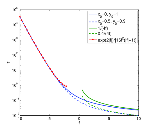
Figure 4: The mean coalescence time $\tau(x_{0},y_{0})$ as a function of the dimensionless force $f$ for two different initial conditions $x_{0}=0,\,y_{0}=1$ (full line) and $x_{0}=0.5,\,y_{0}=0.9$ (dashed line). The asymptotic analytical results for large positive, i.e. “free fall” case with $\tau=(y_{0}-x_{0})/(4f)$, and negative, i.e. large barrier case of Eq. (75), forces are also shown for comparison.

In the rest of this section we focus on a more detailed study of the two limiting cases, the almost “free fall” $f\gg 1$ and the large barrier $f\ll-1$. For these limiting cases we obtain analytical results from relatively simple assumptions which compare quantitatively well with the full solution. We start with the “free fall” (ff) case where we assume that the large drift towards coalescence dominates the dynamics so that the reflecting boundary conditions can be safely neglected since the typical realizations/trajectories of the stochastic process never reach them. The validity of this assumption depends on the initial conditions and we expect it to be good enough for the walkers starting from initial positions $x_{0},\,y_{0}$ satisfying $\mathrm{min}(x_{0},1-y_{0})\gtrsim 1/f$, i.e. far enough from the boundaries. This, indeed, turns out to be the case, see below and compare the corresponding results in Figs. 3a and 3b.

If the reflecting boundary conditions are neglected the 2-walker Fokker-Planck equation (30a) can be solved by separation of variables. In particular, the reformulation of Eq. (30a) together with conditions (30f) and (30g) in terms of the center-of-mass $(x+y)/2$ and relative $y-x$ variables leads to a separable problem which can be easily solved since the center-of-mass coordinate (cms) just performs a free diffusion while the relative coordinate (rel) satisfies equations analogous to those in Ref. hame (Eq. (7) with c=0 therein). Following a derivation similar to that in Sec. V.1 we arrive at (for details the reader is referred to an upcoming publication nome )

$$\varrho_{\rm ff}(x;t|x_{0},y_{0})=P_{\rm cms}\big{(}\frac{x+y}{2};t\big{|}\frac{x_{0}+y_{0}}{2}\big{)}\pi_{\rm rel}(t|y_{0}-x_{0}),$$ (66)

with

$$P_{\rm cms}(u;t\big{|}u_{0})=\frac{1}{\sqrt{2\pi t}}\exp\left(-\frac{(u-u_{0})^{2}}{2t}\right)$$ (67)

being the free diffusion propagator of the center-of-mass coordinate (see Refs. aslangul ; tobiasbob ) and

$$\pi_{\rm rel}(t|y_{0}-x_{0})=\frac{y_{0}-x_{0}}{\sqrt{8\pi t^{3}}}\exp\left(-\frac{(y_{0}-x_{0}-4ft)^{2}}{8t}\right)$$ (68)

the first passage time probability density for the relative coordinate to reach the origin (compare with Eq. (8) in Ref. hame ). Using $\rho(x|x_{0},y_{0})=\int_{0}^{\infty}dt\,\varrho(x;t|x_{0},y_{0})$ and the identity $\int_{0}^{\infty}dt\exp(-a^{2}/(2t)-2b^{2}t)/t^{2}=4b\mathrm{K}_{1}(2ab)/a$ for $a,b>0$ ($\mathrm{K}_{n}(x)$ is the modified Bessel function of the second kind of order $n$) we finally obtain for the coalescence position probability density in the “free fall” limit

$$\begin{split}&\rho_{\rm ff}(x|x_{0},y_{0})=\frac{f(y_{0}-x_{0})\exp[f(y_{0}-x_{0})]\,\mathrm{K}_{1}(2fr)}{\pi\,r},\\ &\text{with}\\ &r\equiv\sqrt{(x-(x_{0}+y_{0})/2)^{2}+(y_{0}-x_{0})^{2}/4}.\end{split}$$ (69)

This function is plotted in Fig. 3a,b for the two different initial conditions for force $f=10$. We can see a rather good agreement between the asymptotic formula (69) and the full result in Fig. 3b. The situation is much worse in Fig. 3a although even there the correspondence is qualitatively quite acceptable. As mentioned above, the reason for the success or failure of the approximation is determined by the initial conditions. Indeed, Fig. 3b corresponds to $f\mathrm{min}(x_{0},1-y_{0})=f(1-y_{0})=1$ where the approximation is expected to become valid while in Fig. 3a the walkers start out right at the boundaries and only an extremely high value of the force could prohibit the walkers from occasionally bumping into the boundaries, especially at the very beginning. Thus, in the case with $x_{0}=0,\,y_{0}=1$ the above approximation is expected to become quantitatively accurate only for very high values of $f$ — numerical estimates reveal that an agreement comparable with that of Fig. 3b is not achieved until about $f\gtrsim 40$. This supports a heuristic guess that the accuracy of the asymptotic analytic expression crosses over from $\exp[-f\mathrm{min}(x_{0},1-y_{0})]$ to $1/f$ when the minimum equals zero.

Now, we turn to the opposite limit of large barrier, i.e. the $f\ll-1$ case. In particular, we want to derive asymptotic expressions for the characteristic coalescence time (which is identified from the results of the full theory as $\tau=1/|\Lambda_{0}|$, cf. the end of Sec. IV.3 and below) and the coalescence position probability density. Clearly, this limit is dominated by the lowest eigenvalue and eigenfunction of the 2-walker problem which means by the two lowest eigenvalues and eigenfunctions of the auxiliary 1-walker problem. Thus we can write, under assumptions of large barrier (lb) and generic initial conditions (to be specified in more detail below), for $P_{\rm lb}(x,y;t|x_{0},y_{0})$,

$$P_{\rm lb}(x,y;t|x_{0},y_{0}) \simeq e^{f(x-y)}e^{-f(x_{0}-y_{0})}e^{(\lambda_{0}+\lambda_{1})t}$$ (70)

$$\times[\psi_{0}(x)\psi_{1}(y)-\psi_{0}(y)\psi_{1}(x)]$$

$$\times[\psi_{0}(x_{0})\psi_{1}(y_{0})-\psi_{0}(y_{0})\psi_{1}(x_{0})],$$

where $\lambda_{0,1}\simeq\pm 4f^{2}e^{-|f|}$ are the lowest eigenvalues satisfying Eq. (54a) and $\psi_{0,1}(x)$ are the corresponding eigenfunctions given by (these are exact expressions for all $f<-2$)

$$\begin{split}\psi_{0}(x)&=\sqrt{\frac{2\lambda_{0}}{\lambda_{0}+2|f|}}\cosh[\sqrt{f^{2}+\lambda_{0}}(x-1/2)],\\ \psi_{1}(x)&=\sqrt{\frac{2|\lambda_{1}|}{\lambda_{1}+2|f|}}\sinh[\sqrt{f^{2}+\lambda_{1}}(x-1/2)]\ .\end{split}$$ (71)

Using these expressions we can study the dependence on the initial conditions and clarify the regime in which the assumption about the dominance of the lowest eigenmode is valid. Utilizing that in the limit $f\ll-1$ the eigenvalues satisfy $|\lambda_{1}|\simeq\lambda_{0}\ll|f|$ we obtain

$$e^{-f(x_{0}-y_{0})}[\psi_{0}(x_{0})\psi_{1}(y_{0})-\psi_{0}(y_{0})\psi_{1}(x_{0})]$$

$$\hskip 34.14322pt\simeq\frac{\lambda_{0}}{|f|}e^{-f(x_{0}-y_{0})}\sinh[|f|(y_{0}-x_{0})]$$

$$\hskip 34.14322pt=\frac{\lambda_{0}}{2|f|}(1-\exp[-2|f|(y_{0}-x_{0})])\ .$$ (72)

Since by assumption $y_{0}>x_{0}$ we see that the evolution depends only exponentially weakly on the initial conditions so that for $y_{0}-x_{0}\gg 1/|f|$ the evolution is essentially independent of the initial conditions as expected in the high barrier limit. Indeed, the above condition just says that the walkers should start out well separated so that the barrier between them is still large (in dimensionless units). In such a case the dynamics is independent of the detailed initial condition or, more precisely, it depends on it only exponentially weakly which can safely be neglected. This is the regime in which the lowest eigenmode theory of Eq. (70) is sufficient as we will demonstrate below.

If we calculate $\varrho(x;t|x_{0},y_{0})$ from Eq. (59) in the limit $f\ll-1,\,y_{0}-x_{0}\gg 1/|f|$ we obtain

$$\begin{split}\varrho_{\rm lb}(x;t|x_{0},y_{0})&\simeq\frac{\lambda_{0}}{|f|}e^{(\lambda_{0}+\lambda_{1})t}[\psi_{0}(x)\psi^{\prime}_{1}(x)-\psi_{1}(x)\psi^{\prime}_{0}(x)]\\ &\simeq\frac{\lambda_{0}^{2}}{|f|}e^{(\lambda_{0}+\lambda_{1})t}\Big{\{}1-\frac{\lambda_{0}}{2f^{2}}\cosh[2|f|(x-1/2)]\Big{\}}.\end{split}$$ (73)

Now integrating over time and taking into account that $\lambda_{0}\simeq 4f^{2}e^{-|f|}$ and $\lambda_{0}+\lambda_{1}\equiv\Lambda_{0}\simeq-16f^{2}(|f|-1)e^{-2|f|}<0$ we get for $\rho(x|x_{0},y_{0})=\int_{0}^{\infty}dt\,\varrho(x;t|x_{0},y_{0})$

$$\rho_{\rm lb}(x|x_{0},y_{0}) \simeq \frac{|f|}{|f|-1}\Big{(}1-2e^{-|f|}\cosh[2|f|(x-1/2)]\Big{)}$$ (74)

$$= \frac{1}{1-\frac{1}{|f|}}\Big{(}1-e^{-2|f|x}-e^{-2|f|(1-x)}\Big{)}.$$

This clarifies that $\rho_{\rm lb}(x|x_{0},y_{0})$ is properly normalized to one within exponential precision, $\int_{0}^{1}dx\,\rho_{\rm lb}(x|x_{0},y_{0})=1+\mathcal{O}\left(e^{-2|f|}\right)\simeq 1$ , which finally proves the self-consistency of the lowest eigenmode approximation. The curves for the case $f=-10$ in Fig. 3a,b calculated by the full theory are practically indistinguishable from that given by the approximate expression (74) (which is an explicit illustration of the initial-condition independence). In a straightforward manner it also follows that the mean coalescence time is given by the inverse lowest eigenvalue $1/|\Lambda_{0}|$ since for $\varrho_{\rm lb}(x;t|x_{0},y_{0})$ in the separable form of Eq. (73) and due to the above normalization condition one immediately gets

$$\tau_{\rm lb}(x_{0},y_{0}) \simeq \int_{0}^{\infty}dt\,t\int_{0}^{1}dx\,\varrho_{\rm lb}(x;t|x_{0},y_{0})$$ (75)

$$= \int_{0}^{\infty}dt\,te^{-|\Lambda_{0}|t}|\Lambda_{0}|\int_{0}^{1}dx\,\rho_{\rm lb}(x|x_{0},y_{0})$$

$$\simeq \frac{1}{|\Lambda_{0}|}\simeq\frac{e^{2|f|}}{16f^{2}(|f|-1)},$$

independent of the initial conditions. All approximate equalities hold up to exponentially small corrections of order $e^{-2|f|}$, which are negligible for $f\ll-1$.

V.3 Summary

We have in Secs. III, IV, and V set up an approximate Fokker-Planck equation scheme for the full problem of two interfaces moving in a block DNA-stretch with a barrier region separating two soft zones. While the full problem can be viewed as two discrete random walkers in different potentials with an imposed vicious boundary condition, the approximate Fokker-Planck equation describes two continuous random walkers in opposite linear potentials keeping the imposed viciousness condition. The four assumptions leading to the Fokker-Planck equation were introduced in Sec. III and their validity will be discussed favorably in Sec. VII when we compare the Fokker-Planck results with the direct evaluation of the full discrete problem using the master equation approach presented in the next section.

The main outcome of the Fokker-Planck approach are the general results for the coalescence time density $\pi(t)$ (examples will be shown in Sec. VII), and the numerical and analytic expressions for the mean meeting time $\tau$ (shown in Fig. 4) as well as the probability density $\rho$ for the meeting position (shown in Fig. 3). All results are expressed through the dimensionless force $f$, which in terms of the parameters from an experimental setup reads

$$f=\frac{N(u_{b}-1)}{u_{b}+1},$$ (76)

making comparison with values obtained from experiments straightforward.

Finally, a remark on why one should consider the continuous approach over the complete, discrete master equation approach is in order. Namely, for DNA-stretches of length $N$ the discrete master equation approach involves diagonalization of matrices of the order $N^{2}\times N^{2}$, setting computational limitations on $N$ and a new diagonalization is needed for each parameter set. The Fokker-Planck approach may therefore provide additional insight for very long DNA stretches as we showed here by discussing the physical quantities of meeting position and meeting time.

VI Complete discrete approach: the master equation

In this section, we develop a master equation framework for the bubble coalescence. In contrast to the previous treatment, we explicitly allow the soft zones to zip close from the two ends of the barrier region. It will turn out that in some cases this only has a minor effect. A detailed comparison with the continuum Fokker-Planck equation approximation is shown in the next section.

We consider the same segment of double-stranded DNA with $M=N_{L}+N+N_{R}$ internal base-pairs, clamped open at both ends according to Fig. 1. However, in contrast to the approximations imposed in the Fokker-Planck approximation, we now allow for explicit closure of the soft regions, necessitating the consideration of a sequence-dependence of the local DNA stability, in contrast to the previous discussion, where we assumed that the two bubble domains are always remaining open.

Note that in this section our notation differs from the scheme introduced above, first, in order to keep the notation of this section consistent with previous references on the same method JPC ; tobiasprl ; tobiasbj ; tobiasrc ; tobiaspre , and second, to be able to incorporate zipping/unzipping of base pairs in the soft zones, as well. We denote by $x_{L}=X+N_{L}$ ($x_{R}=Y+N_{L}$) the position of the rightmost (left-most) open basepair in the left (right) open region, see Fig. 1, where $x_{L,R}\in[0,M]$. The positions $x_{L}$ and $x_{R}$ of the two zipper forks are stochastic variables and the aim is to understand how these variables evolve in time without taking the continuum limit and using the approximations introduced in Sec. III. We note that an equivalent set of variables are $x_{L}$ and the clamp size $m$, that are related through

$$m=x_{R}-x_{L}.$$ (77)

In the master equation formulation below we will use $x_{L}$ and $m$ as the dynamic variables, and for completeness we state the transition rates, Eqs. (4), (5), (7), (8), and (12), (13) expressed in the new variables: The reflecting boundary conditions are

$$t_{L}^{-}(x_{L}=0,m)=t_{R}^{+}(x_{L},m=M-x_{L})=0.$$ (78)

Once the clamp is completely unzipped, i.e. the state $m=0$ is reached, we assume that the clamp will not be able to reform for a long time, and we impose the absorbing conditions

$$t_{L}^{-}(x_{L},m=0)=t_{R}^{+}(x_{L},m=0)=0.$$ (79)

The transition rates at the interior of the DNA stretch is

$$t^{-}_{L}(x_{L},m) = \frac{1}{2}\mathcal{K}(x_{L}),$$ (80)

$$t^{+}_{R}(x_{L},m) = \frac{1}{2}\mathcal{K}(M-m-x_{L}),$$ (81)

$$t_{L}^{+}(x_{L},m) = \frac{1}{2}\mathcal{K}(x_{L}+1)u(x_{L}+1)s(m),$$ (82)

$$t_{R}^{-}(x_{L},m) = \frac{1}{2}\mathcal{K}(M-m-x_{L}+1)u(x_{R}-1)$$ (83)

$$\times s(M-m-x_{L}),$$

where $x_{R}=x_{L}+m+1$, $s(q)=\{(q+1)/(q+2)\}^{c}$ and $\mathcal{K}(q)=kq^{-\mu}$. The properties of the four transfer coefficients above are summarized in Table 1.

	$\Delta x_{L}$	$\Delta x_{R}$	$\Delta m$	Eq.
$t_{L}^{+}(x_{L},m)$	$1$	$0$	$-1$	(80)
$t_{R}^{-}(x_{L},m)$	$0$	$-1$	$-1$	(81)
$t_{L}^{-}(x_{L},m)$	$-1$	$0$	$1$	(82)
$t_{R}^{+}(x_{L},m)$	$0$	$1$	$1$	(83)

Table 1: Properties of the transfer coefficients. The quantity $\Delta x_{L}$ ($\Delta x_{R})$ denotes the change in fork position $x_{L}$ ($x_{R}$) under the action of the transfer coefficients. Similarly $\Delta m$ denotes the change in clamp size $m$.

Denote by $P(x_{L},m,t|x_{L}^{\prime},m^{\prime})$ the conditional probability to find the system in state $(x_{L},m)$ at time $t$, given the initial condition $(x_{L}^{\prime},m^{\prime})$ at time $t=0$. With the short-hand notation $P(x_{L},m,t)=P(x_{L},m,t|x_{L}^{\prime},m^{\prime})$ the dynamics is described by the master equation

$$\frac{\partial}{\partial t}P(x_{L},m,t)=$$

$$t_{L}^{+}(x_{L}-1,m+1)P(x_{L}-1,m+1,t)$$

$$+t_{L}^{-}(x_{L}+1,m-1)P(x_{L}+1,m-1,t)$$

$$-\left[t_{L}^{+}(x_{L},m)+t_{L}^{-}(x_{L},m)\right]P(x_{L},m,t)$$

$$+t_{R}^{+}(x_{L},m-1)P(x_{L},m-1,t)$$

$$+t_{R}^{-}(x_{L},m+1)P(x_{L},m+1,t)$$

$$-\left[t_{R}^{+}(x_{L},m)+t_{R}^{-}(x_{L},m)\right]P(x_{L},m,t).$$ (84)

This equation states that the probability for the clamp size can change in 8 different ways: the terms with a plus-sign correspond to jumps to the state $\{x_{L},m\}$, and the terms with a minus-sign correspond to jumps from the state $\{x_{L},m\}$.

A standard approach to the master equation (84) is the spectral decomposition van_Kampen ; Risken

$$P(x_{L},m,t)=\sum_{p}c_{p}(x_{L}^{\prime},m^{\prime})Q_{p}(x_{L},m)\exp(-\eta_{p}t),$$ (85)

in terms of the eigenvalues $\eta_{p}$ and eigenvectors $Q_{p}(x_{L},m)$. The expansion coefficients $c_{p}(x_{L}^{\prime},m^{\prime})$ are obtained from the initial condition. As in the previous section, we will assume the system initially to be in the state where all bps in the soft zone are broken and all bps in the barrier region are closed.

The eigenvalue equation corresponding to Eq. (84) becomes

$$t_{L}^{+}(x_{L}-1,m+1)Q_{p}(x_{L}-1,m,t)$$

$$+t_{L}^{-}(x_{L}+1,m-1)Q_{p}(x_{L}+1,m-1,t)$$

$$-\left[t_{L}^{+}(x_{L},m)+t_{L}^{-}(x_{L},m)\right]Q_{p}(x_{L},m,t)$$

$$+t_{R}^{+}(x_{L},m-1)Q_{p}(x_{L},m-1,t)$$

$$+t_{R}^{-}(x_{L},m+1)Q_{p}(x_{L},m+1,t)$$

$$-\left[t_{R}^{+}(x_{L},m)+t_{R}^{-}(x_{L},m)\right]Q_{p}(x_{L},m,t)$$

$$\hskip 22.76228pt=-\eta_{p}Q_{p}(x_{L},m,t).$$ (86)

The eigenvectors satisfy the orthogonality relation van_Kampen

$$\sum_{m=1}^{M}\sum_{x_{L}=0}^{M-m}\frac{Q_{p}(x_{L},m)Q_{p^{\prime}}(x_{L},m)}{P^{\rm eq}_{r}(x_{L},m)}=\delta_{pp^{\prime}},$$ (87)

where

$$P_{r}^{\rm eq}(x_{L},m)=\mathscr{Z}(x_{L},m)/\mathscr{Z},$$ (88)

with

$$\mathscr{Z}=\sum_{x_{L},m}Z(x_{L},m),$$ (89)

being the partition coefficient in the variable $x_{L}$ and $m$ (neglecting a common $\sigma_{0}^{2}$-factor, where $\sigma_{0}$ is the bubble initiation parameter), and where

$$\mathscr{Z}(x_{L},m) = \prod_{\tilde{x}_{L}=0}^{x_{L}}u(\tilde{x}_{L})\prod_{\tilde{x}_{R}=m+x_{L}+1}^{M+1}u(\tilde{x}_{R})$$ (90)

$$\times(1+x_{L})^{-c}(M-m-x_{L}+1)^{-c},$$

see Eqs. (1)-(3). From the eigenvalues and eigenvectors of Eq. (86) any quantity of interest may be constructed. In the following subsection we calculate the coalescence time density. How to set up the master equation for numerical purposes is presented in detail in App. B. Alternatively, the master equation (84) can be solved by direct stochastic simulations such as, e.g. the Gillespie algorithm introduced in App. C and used in Sec. VII.

VI.1 Coalescence time density

The (survival) probability that the absorbing boundary at $m=0$ has not yet been reached up to time $t$ is

$$\mathscr{S}(x_{L}^{\prime},m^{\prime},t)=\sum_{m=1}^{M}\sum_{x_{L}=0}^{M-m}P(x_{L},m,t|x_{L}^{\prime},m^{\prime}).$$ (91)

The probability that the absorbing boundary is reached within the time interval $[t,t+dt]$ (namely, the coalescence time density corresponding to the first passage problem) is

$$\rho(x_{L}^{\prime},m^{\prime},t)dt = \mathscr{S}(x_{L}^{\prime},m^{\prime},t)-\mathscr{S}(x_{L}^{\prime},m^{\prime},t+dt)$$ (92)

$$= -\left(\frac{\partial}{\partial t}\mathscr{S}(x_{L}^{\prime},m^{\prime},t)\right)dt.$$

This expression is positive, as $\mathscr{S}$ is decreasing with time. To express the coalescence time density in terms of the eigenvalues and eigenfunctions, we introduce the eigenmode expansion (85) into equation (92), yielding

$$\rho(x_{L}^{\prime},m^{\prime},t)=\sum_{p}\eta_{p}c_{p}(x_{L}^{\prime},m^{\prime})\exp(-\eta_{p}t),$$ (93)

with coefficients

$$c_{p}(x_{L}^{\prime},m^{\prime})=\frac{Q_{p}(x_{L}^{\prime},m^{\prime})}{P_{r}^{\rm eq}(x_{L}^{\prime},m^{\prime})}\sum_{m=1}^{M}\sum_{x_{L}=0}^{M-m}Q_{p}(x_{L},m).$$ (94)

We have above made use of the orthonormality relation (87) in order to express $c_{p}(x_{L}^{\prime},m^{\prime})$ in terms of the initial probability density $P(x_{L},m,0|x_{L}^{\prime},m^{\prime})$, and used the fact that this general initial condition takes the explicit form $P(x_{L},m,0|x_{L}^{\prime},m^{\prime})=\delta_{x_{L},x_{L}^{\prime}}\delta_{m,m^{\prime}}$. Eq. (93) is the discrete counterpart of the continuous result derived in Ref. Gardiner , and expresses the coalescence time density (for any given initial condition, specified by $m^{\prime}$ and $x_{L}^{\prime}$) in terms of the eigenvalues and eigenvectors of Eq. (86).

VII Comparison between the full master equation and the Fokker-Planck approximation

In this section, we investigate the validity of the assumptions presented in Sec. III leading to the Fokker-Planck continuum approximation. This is done by comparing the results for the coalescence time densities, $\pi(t)$, with the results obtained from the full discrete master equation approach. In the next section, Sec. VIII, we discuss the relevance for biological experiments.

In all examples below the two walkers move between $[0,N]$ in the Fokker-Planck description and between $[-N_{L},N+N_{R}]$ in the master equation setup. That is, in the master equation approach we explicitly allow zipping of base pairs in the two soft zones. As initial conditions we use $X_{0}=0$ and $Y_{0}=N$ throughout this section.

VII.1 The continuum approximation

The continuum assumption (iv) implies that the inherently discrete nature of the DNA structure - both in terms of stacking and hydrogen bonds - can be approximated by the diffusive behavior of two continuous variables. To get the Fokker-Planck description one has to consider the limit $a\rightarrow 0$ with $a$ being the length between effective bonds in the base pairs. In practice this limit is obtained by

$$\frac{\text{bond distance}}{\text{total segment length}}\rightarrow 0,$$

i.e. by increasing the width of the barrier region. The question is addressed in a setup with open soft zones, i.e. $u_{s}\gg 1$, and varying barrier lengths, $N$. To have perfectly reflecting boundary conditions we set $N_{L}=N_{R}=0$ in the master equation setup.

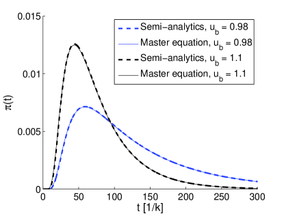
Figure 5: Coalescence time probability density for barrier width $N=20$ and temperature below and above $T_{b}$, with $u_{b}=0.98$ and $u_{b}=1.1$, respectively. To exclude other effects, the lengths of the soft zones are zero, $N_{L}=N_{R}=0$, i.e., these are assumed to be always open, and $c=\mu=0$.

Fig. 5 shows that it requires a relatively small number of base pairs ($\sim 20$) before the continuum approximation is reasonable, independently of the temperature. Barrier regions of this length are in principle accessible experimentally so the continuum approximation appears to be well-justified.

VII.2 Open soft zones

The first assumption, (i), states that the soft zones are always open, i.e. that the random walkers are reflected at the interfaces between the barrier region and the soft zones.

To eliminate other effects than the effect of the introduction of the reflecting boundary conditions at the ends of the barrier region, we consider a DNA stretch of length 25, so that the continuum approximation is justified, and set $c=\mu=0$ in order to exclude effects originating from the entropy factor and the hook exponent. We compare this to the results from the full master equation including the soft zones.

Fig. 6 shows the coalescence time density $\pi(t)$ for varying lengths of the soft zones for temperatures above and below the melting temperature of the barrier region. Apparently, the length dependence is rather weak as long as the soft zones serve as hard enough boundaries, i.e. for large enough $u_{s}\gtrsim 5$. For smaller $u_{s}$ the soft-zone-length dependence is relevant as the two bubble corners venture more frequently into the soft zones. This, however, implies the breaking of the assumptions for the applicability of our Fokker-Planck description as revealed in the figure. Thus, the length of the soft zones itself is not important if $u_{s}$ is large enough and $c=\mu=0$. Systematic assessment of these conditions is given below.

Fig. 7 shows $\pi(t)$ as a function of $u_{s}$ for $N_{L}=N_{R}=20$, i.e. the soft zones are so long the two forks essentially never reach the outer clamps. That this is indeed the case can be qualitatively investigated using the Gillespie-scheme presented in App. C, giving access to real-time trajectories of the two random walkers in a potential landscape including both the barrier region and the soft zones. This is shown in Fig. 8 which confirms that excursions into the soft zones are progressively suppressed with increasing $u_{s}$. In Fig. 7 we have only included the case $u_{b}<1$, i.e., when the barrier region indeed acts as a barrier, and consequently the effect of the soft zones is more pronounced. The discrepancies between the Fokker-Planck and the master equation approach become distinct for $u_{s}\simeq 1$ whereas for $u_{s}\gtrsim 5$ the agreement between the approaches becomes reasonable. Difference between $u_{s}$ and $u_{b}$ of this magnitude can indeed be achieved in realistic experimental setups, as shown in the next section.

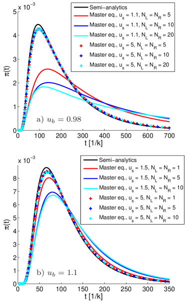
Figure 6: Coalescence time density for varying soft zone lengths and fixed length of the barrier $N=25$. Included are plots for $u_{b}=0.98$ (upper) and $u_{b}=1.1$ (lower), i.e. for temperatures below and above the melting temperature of the barrier, respectively. Furthermore, $c=\mu=0$.

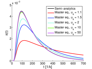
Figure 7: Coalescence time density for $N=25$, $N_{L}=N_{R}=20$, $u_{b}=0.98$ and different values of $u_{s}$. Furthermore, $c=\mu=0$.

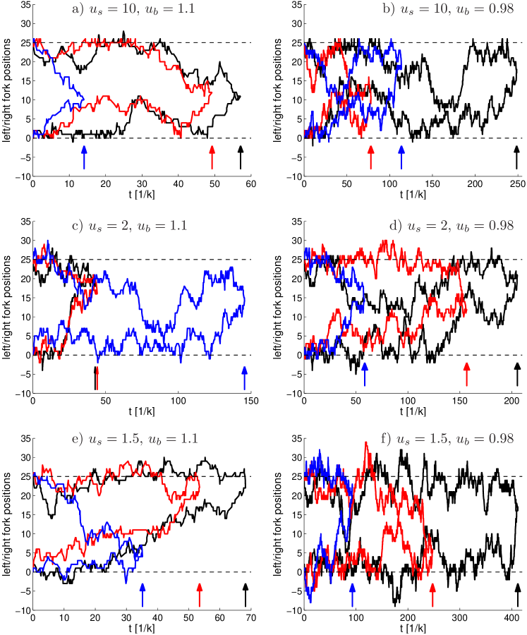
Figure 8: Single trajectories for the two zipper forks, based on the Gillespie (Monte Carlo) algorithm presented in App. C. The values of $u_{b}$ and $u_{s}$ are stated in the figures. The other parameters are $N_{L}=N_{R}=20$, $N=25$, $c=\mu=0$. The dashed horizontal lines mark the boundaries between the barrier region and the soft zones, and the arrows indicate the ends of the sampled trajectories.

VII.3 Loop Entropy and Hook factors

The general rates defined in Sec. II include both the entropy loss factor and the hook factor. Both depend on the length $q$ of the bubble, and for both their relative influence diminishes for increasing bubble lengths. In the Fokker-Planck description both factors are omitted, which are the assumptions (ii) and (iii). These assumptions are valid for long bubbles, which can be obtained by having long soft zones and keeping the temperature far above the melting temperature of the soft zones, i.e. $u_{s}\gg 1$.

Fig. 9 studies the effect of the loop exponent $c$ on the coalescence time density $\pi(t)$ for a fixed length of the barrier region, $N=15$ and varying the lengths of the soft zones. Even for soft zones of length $N_{L}=N_{R}=30$ there is a substantial influence of the loop entropy factor, making long soft zones a requirement in experimental realizations which should agree reasonably with the Fokker-Planck approach.

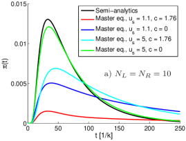
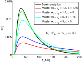
Figure 9: Coalescence time density $\pi(t)$ for fixed barrier width $N=15$, and varying the length of the soft zones, $N_{L}=N_{R}=10$ in Fig. 9 and $N_{L}=N_{R}=30$ in Fig. 9, respectively. The other parameters are $u_{b}=0.98$, $\mu=0$.

The hook factor leads to a decrease in the rate constant $k$, $k\rightarrow kq^{-\mu}$ where $q$ is the length of a given bubble, so introducing the hook exponent $\mu>0$ leads to a considerable and bubble-length-dependent decrease of the transition rates, see Fig. 10. However, for sufficiently large bubbles, the rate is roughly constant and introducing a renormalized rate constant $\tilde{k}=kL^{\mu}$ can compensate for this effect. Here $L$ is a characteristic bubble size. If the temperature is kept well above the melting temperature of the soft zones, and the length of the soft zones are much longer than the barrier, $L$ is well approximated by the length of the soft zones, $L\simeq N_{L/R}$. In Fig. 10 we illustrate the effect of a renormalized rate constant (with $L=53$ being the best fit) together with the standard rate coefficient $k=1$.

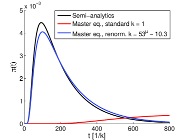
Figure 10: Coalescence time density $\pi(t)$ for non-vanishing hook exponent $\mu=0.588$, $N_{L}=N_{R}=50$ and $N=25$ for the barrier case, $u_{b}=0.98$. The results are shown with and without the renormalized rate constant $k$, where we have used $\tilde{k}=53^{0.588}\simeq 10.3$. The other parameters are $u_{s}=10$ and $c=0$.

In conclusion, both the influence of the loop entropy factor and the hook exponent can be eliminated by keeping the length of the soft zones sufficiently long and using a renormalized value for the rate constant $k$.

VIII Relevance for single molecule experiments

Relevant for the separation of statistical weights are the empirical relations krueger

$$T_{m}^{AT} = (355.55+7.95\ln[\mathrm{Na}^{+}])K$$ (95a)

$$T_{m}^{GC} = (391.55+4.98\ln[\mathrm{Na}^{+}])K,$$ (95b)

which give the melting temperatures of GC and AT pairs in terms of the (intermediate) salt-concentration in the solvent obtained from melting experiments kamanetskii71 . Note that the value of $T_{m}^{AT}$ stems from an average over all possible combinations of AT and TA base pairs krueger ; if only TA/AT and AT/TA pairs are interchangeably used the value of $T_{m}^{AT}$ can be lowered further. The above relations can be translated into free-energy differences by $\Delta G=\Delta S(T_{m}-T)$, where $\Delta S=-24.85$cal/(mol K) yakovchuk06 . Eqs. (95a), (95b) contain contributions from both base stacking and hydrogen bonding, and is thus the melting temperature suitable for our situation. It has been shown that the dependence on salt-concentration lies in the stacking term yakovchuk06 and not as previously thought in the hydrogen bonding term protozanova04 . The stacking is a combination of hydrophobic, electrostatic (screening of the negatively charged phosphate groups), and dispersive interactions but there is no apparent consensus on which term is the dominant one yakovchuk06 . At high salt-concentrations $\sim 1-5$M the temperature dependence levels off due to a decrease in the hydrophobic effect; with most water molecules tied up in the solvation of ions, the entropy decrease involved in base stacking is small schildkraut65 .

The melting temperature of AT bonds has a stronger dependence on salt-concentration, so we can increase the ratio $u_{AT}/u_{GC}$ by decreasing the salt-concentration. A further benefit is a lowering of the melting temperatures thus enabling experiments well below $T_{m}^{GC}\sim 100^{o}$C, which is the case when $[\mathrm{Na}^{+}]=0.1$M, the standard concentration in electrophoresis experiments. High temperatures have practical disadvantages such as formation of air bubbles and increased evaporation of solvent molecules schildkraut65 .

Most relevant experiments on DNA have been conducted at $\sim 0.1$M salt-concentration. Those specifically looking at the salt dependence of the melting temperature work in the range $\sim 0.01-1$M. A conservative estimate of $[\mathrm{Na}^{+}]=0.01$M gives $u_{GC}\sim 1$ and $u_{AT}\simeq 6$ at $T\simeq 95^{o}$C, which is sufficient for the Fokker-Planck approximation to be valid.

Concerning the possible length of a DNA construct it should be reasonable to work with segments up to $100-200$ bps. In a setup combining fluorescence correlation spectroscopy and fluorescence quenching, as introduced in Ref. altan , the DNA is free to diffuse around in the solution. In this case the limiting factor is the time it takes for the quencher to diffuse in and out of the confocal volume.

Practically the experimental method of choice may be a dual optical tweezers setup in which the DNA construct, via some handles of double-stranded DNA, is connected to two beads held in place by the tweezers. While this allows to keep the DNA construct in place the force exerted on the chain is relatively small. However this would allow direct observation of the construct avoiding diffusional correction. The centre of the barrier region could be decorated with either a fluorophore-quencher pair, or markers such as quantum dots or small gold beads that can be visualized by a microscope. The influence of the attached markers should decrease with longer barrier length. Having this setup in a flow cell the system could be triggered by flushing in a solution with either different temperature or salt concentration. This can be done relatively quickly gijs . Once the two initial bubbles are thereby created it should be possible to measure the coalescence time calculated herein. Repeating the experiment would produce the distribution of coalescence times, from which important system parameters can be inferred. Decorating the barrier region with several, sufficiently small, markers would, in principle, allow one to measure the position of the coalescence.

IX Final conclusions

Single molecule techniques give us increasing insight into the behavior, equilibrium and dynamic, of biopolymers. Of particular and outstanding interest is DNA, due to its importance in biological contexts as well as its role as a model biopolymer. In order to extend our knowledge about the biological function of DNA it is crucial to quantify and understand the denaturation behavior of DNA at the single molecule level, its sequence dependence and, ultimately, its relevance to genetic processes such as transcription initiation. A major question hereby concerns the dynamics of transient DNA denaturation bubbles.

While first single molecule fluorescence correlation experiments have demonstrated the feasibility of monitoring the fluctuations of a single bubble, some questions remain about the model system and the explicit setup used in these experiments. In particular, the obtained time scales for base pair zipping and unzipping as well as the influence of the attached fluorophore-quencher pair remain under debate.

Here we suggest an alternative model for accessing DNA stability parameters and basepair (un-zipping) constants: in our model system DNA bubbles in two AT-rich regions are formed and separated by a more stable GC-rich barrier region. The coalescence behavior of the two DNA bubbles across the barrier region is then studied. We show that the stability parameters for bubble and barrier regions can indeed be chosen sufficiently different to allow preparation of the DNA construct in the proposed fashion, by the proper adjustment of temperature and/or salt concentration. Once coalesced the newly created single bubble is stabilized against immediate reclosure of the barrier region both dynamically and due to the release of the boundary free energy corresponding to one cooperativity factor $\sigma_{0}$. Appropriate fluorophore-quencher tagging of the barrier region basepairs should therefore allow for the direct observation of the bubble merging dynamics.

Apart from the relevance of the investigated system for understanding the dynamics of DNA and its biological function, the mathematical description presented here is of interest for its own sake as it corresponds to a previously unsolved case of two vicious random walkers in opposite linear potentials. We established the solution of this problem by solving a bivariate Fokker-Planck equation (continuum limit of the discrete master equation description) analytically. In a careful analysis we showed under what conditions the Fokker-Planck approach is valid and what deviations one would expect for realistic systems. Furthermore, the analytic results were explained using qualitative arguments and corroborated using stochastic simulations.

Appendix A Calculation of $\tilde{p}(x;t|x_{0})$ via Laplace transform

In this appendix we present a detailed calculation of the single-walker auxiliary density $\widetilde{p}(x;t|x_{0})$ satisfying Eq. (49) together with the boundary conditions Eqs. (37a) and (37b), as well as the initial condition $\widetilde{p}(x;t=0|x_{0})=\delta(x-x_{0})$. $\widetilde{p}(x;t|x_{0})$ solves the Schrödinger equation

$$\frac{\partial}{\partial t}\widetilde{p}(x;t|x_{0})=\left[\frac{\partial^{2}}{\partial x^{2}}-f^{2}\right]\widetilde{p}(x;t|x_{0}),$$ (96)

that, after a Laplace transform and some rearrangement becomes

$$\left[\frac{\partial^{2}}{\partial x^{2}}-k(z)^{2}\right]\tilde{p}(x;z|x_{0})=-\delta(x-x_{0}),$$ (97)

with $k(z)=\sqrt{z+f^{2}}$ (we skip the explicit $z$-dependence in the formulas from now on).

Consider first the solution of equation

$$\left[\frac{\partial^{2}}{\partial x^{2}}-k^{2}\right]g(x,x_{0})=0,$$ (98)

for $x<x_{0}$ with boundary condition (37a), and for $x>x_{0}$ with boundary condition (37b). The solutions are

$$g(x,x_{0})=\left\{\begin{array}[]{ll}C_{<}\left(\kappa e^{kx}+e^{-kx}\right),&x<x_{0},\\[5.69046pt] C_{>}\left(e^{kx}+\kappa e^{2k}e^{-kx}\right),&x>x_{0},\end{array}\right.$$ (99)

with $\kappa\equiv(k+f)/(k-f)$.

The solution of Eq. (97) can now be found by the ansatz

$$\widetilde{p}(x;z|x_{0})=$$

$$\left\{\begin{array}[]{ll}C\left(\kappa e^{kx}+e^{-kx}\right)\left(e^{kx_{0}}+\kappa e^{2k}e^{-kx_{0}}\right),&x<x_{0},\\[5.69046pt] C\left(\kappa e^{kx_{0}}+e^{-kx_{0}}\right)\left(e^{kx}+\kappa e^{2k}e^{-kx}\right),&x>x_{0},\end{array}\right.$$ (102)

such that

$$\widetilde{p}(x;z|x_{0})=C\left\{\kappa\left(e^{k(x+x_{0})}+\kappa e^{2k}e^{-k|x-x_{0}|}\right)\right.$$

$$\left.+e^{k|x-x_{0}|}+\kappa e^{2k}e^{-k(x+x_{0})}\right\},$$ (103)

where $C$ is determined from the jump condition by integrating Eq. (97)

$$-1 = \lim_{\epsilon\rightarrow 0^{+}}\int_{x_{0}-\epsilon}^{x_{0}+\epsilon}\left[\frac{\partial^{2}}{\partial x^{2}}-f^{2}\right]\widetilde{p}(x;z|x_{0})dx$$ (104)

$$= \lim_{\epsilon\rightarrow 0^{+}}\left\{\frac{\partial}{\partial x}\widetilde{p}(x;z|x_{0})\Big{|}_{x_{0}+\epsilon}-\frac{\partial}{\partial x}\widetilde{p}(x;z|x_{0})\Big{|}_{x_{0}-\epsilon}\right\}$$

$$= 2kC\left(1-\kappa^{2}e^{2k}\right).$$

Here, it has been used that $\widetilde{p}(x;z|x_{0})$ is continuous.

Appendix B Implementation of the discrete master equation

To solve the eigenvalue equation (86) by a numerical scheme, it is convenient to replace the two-dimensional grid points $(x_{L},m)$ by a one-dimensional coordinate $s$ counting all lattice points, compare with JPC . We choose the enumeration illustrated in figure 11.

Figure 11: Enumeration scheme for the numerical analysis: The two-dimensional grid points $(x_{L},m)$ are replaced by a one-dimensional running variable $s$. See text for details.

From this figure we notice that $m\in[1,M]$ and $x_{L}\in[0,M-m]$. An arbitrary $s$-point can be obtained from a specific $(x_{L},m)$ according to:

$$s=(m-1)M-\frac{(m-1)(m-2)}{2}+x_{L}.$$ (105)

From this relation we notice that the maximum $s$ value is

$$S={\rm max}\{s\}=\frac{M(M+1)}{2}-1,$$ (106)

i.e., the size of the relevant $W$-matrix (see below) scales as $M^{2}/2$. Expression (105) allows us to change the transfer coefficients to the $s$-variable, $t^{\pm}_{L/R}(x_{L},m)\rightarrow t^{\pm}_{L/R}(s)$, using the explicit expressions (80), (81), (82) and (83) for the transfer coefficients, together with the boundary conditions in equations (78) and (79). From equation (105) and Fig. 11 we notice that [compare with Eq. (86)]

$$s|_{x_{L}-1}^{m+1} = s|_{x_{L}}^{m}+M-m,\ {\rm for}\ x_{L}\geq 1,$$

$$s|_{x_{L}+1}^{m-1} = s|_{x_{L}}^{m}-(M-m+1),\ {\rm for}\ m\geq 2,$$

$$s|_{x_{L}}^{m-1} = s|_{x_{L}}^{m}-(M-m+2),\ {\rm for}\ m\geq 2,$$

$$s|_{x_{L}}^{m+1} = s|_{x_{L}}^{m}+M-m+1,$$

$$\ {\rm for}\ x_{L}\leq M-(m+1)\ \&\ m\leq M-1,$$

Eq. (86) can then be written in matrix form as

$$\sum_{s^{\prime}}W(s,s^{\prime})Q_{p}(s^{\prime})=-\eta_{p}Q_{p}(s),$$ (108)

where explicitly the matrix-elements are

$$W(s,s+M-m) = t_{L}^{+}(s+M-m),$$

$${\rm for}\ s\pitchfork x_{L}\geq 1,$$

$$W(s,s-[M-m+1]) = t_{L}^{-}(s-[M-m+1]),$$

$${\rm for}\ s\pitchfork m\geq 2$$

$$W(s,s-[M-m+2]) = t_{R}^{+}(s-[M-m+2]),$$

$${\rm for}\ s\pitchfork m\geq 2,$$

$$W(s,s+M-m+1) = t_{R}^{-}(s+M-m+1),$$

$${\rm for}\ s\pitchfork x_{L}\leq M-(m+1)$$

$$\&\ m\leq M-1,$$

$$W(s,s) = -(t_{L}^{+}(s)+t_{L}^{-}(s)$$ (109)

$$+t_{R}^{+}(s)+t_{R}^{-}(s)),$$

and the remaining matrix elements are equal to zero. We have introduced the notation $s\pitchfork$ with the meaning “$s$ is to be taken for”. The problem at hand is that of determining the eigenvalues and eigenvectors of the $(S+1)\times(S+1)$-matrix $W$ above. The coalescence time density is then calculated from Eqs. (93) and (94). In terms of the running variable $s$, see Eq. (105), and the $W$-matrix defined in equation (109) the detailed balance conditions (10) and (11) become

$$W(s,s^{\prime})\mathscr{Z}(s^{\prime})=W(s^{\prime},s)\mathscr{Z}(s).$$ (110)

The orthogonality relation, Eq. (87), becomes

$$\sum_{s}\frac{Q_{p}(s)Q_{p^{\prime}}(s)}{P_{r}^{\rm eq}(s)}=\delta_{p,p^{\prime}}.$$ (111)

Convenient checks of the numerical results then include: (i) The eigenvalues should be real and negative (so that $\eta_{p}>0$); (ii) The eigenvectors should satisfy the orthonormality relation, Eq. (111).

Appendix C Stochastic simulation of bubble coalescence

In this Section we give a brief introduction to the stochastic simulation of DNA-breathing, for details we refer to Ref. suman . We apply the Gillespie algorithm introduced in $1976$ as a stochastic approach to the study of chemical reactions gillespie76 .

Following the schematic of Fig. 1, we simulate the dynamics of the two zipping forks separating the two initial bubble domains from the barrier region. As each fork can either zip or unzip, the system is described by the four different rates, $t^{\mu}_{\nu}$, where $\mu\in\{+,-\}$, and $\nu\in\{L,R\}$. Given these rates, we assume that the statistical weight for a given event, $\{\mu,\nu\}$, to occur in a time interval $[t,t+\delta t]$ is $t^{\mu}_{\nu}\delta t$. Then the idea of the Gillespie scheme is the following gillespie76 : The probability that nothing happens in the time interval $[t,t+\tau]$, and that in the following interval $[t+\tau,t+\tau+d\tau]$ an event of type $\{\mu,\nu\}$ occurs, is the so-called reaction probability density

$$P(\tau,\mu,\nu)d\tau=P_{0}(\tau)t^{\mu}_{\nu}d\tau.$$ (112)

To determine the probability $P_{0}(\tau)$ that no event happens within $[t,t+\tau]$, this interval is divided into $K$ spans of duration $\epsilon=\tau/K$. The probability that no event occurs in the first subinterval $[t,t+\epsilon]$ is then

$$\prod_{\mu,\nu}\left[1-t^{\mu}_{\nu}\epsilon\right]=1-\sum_{\mu,\nu}t^{\mu}_{\nu}\epsilon+\mathcal{O}(\epsilon^{2}).$$ (113)

Treating the remaining intervals similarly produces an expression for $P_{0}$,

$$P_{0}(\tau) = \left[1-\sum_{\mu,\nu}t^{\mu}_{\nu}\epsilon+\mathcal{O}(\epsilon^{2})\right]^{K}$$ (114)

$$= \left[1-\sum_{\mu,\nu}t^{\mu}_{\nu}\tau/K+\mathcal{O}(K^{-2})\right]^{K}.$$

Taking the limit $K\rightarrow\infty$ and reinserting in Eq. (112), we find the Poissonian law

$$P(\tau,\mu,\nu)=t^{\mu}_{\nu}\exp\left(-\sum_{\mu,\nu}t^{\mu}_{\nu}\tau\right).$$ (115)

At some given instant of time, $t$, the system is in a certain configuration. The update is performed as follows:
(i) The rates $t^{\mu}_{\nu}$ are calculated according to the configuration.
(ii) A set of random numbers $(\tau,\mu,\nu)$, distributed according to $P(\tau,\mu,\nu)$ in Eq. (115), is drawn from a generator.
(iii) The time is advanced according to $t\rightarrow t+\tau$, and the configuration is updated according to the randomly chosen event $\mu,\nu$.
The steps (i)-(iii) are repeated until a specified stop criterion is fulfilled, in our case the merging of the two initial bubbles. We record the stop time and the final configuration, and a new run is initiated using the same initial condition.

Following Ref. gillespie76 we briefly present how random numbers $\tau$ and $\mu$ can be constructed using numbers drawn from a uniform distribution: Let $P_{c}(\tau^{\prime})$ be some continuous probability density function, e.g., $P_{c}(\tau^{\prime})d\tau$ is the probability for finding a $\tau$ within the interval $[\tau^{\prime},\tau^{\prime}+d\tau]$. The associated probability distribution function is then defined as

$$F_{c}(\tau_{0})=\int_{-\infty}^{\tau_{0}}P_{c}(\tau^{\prime})d\tau^{\prime},$$ (116)

which is the probability of some $\tau$ being less than $\tau_{0}$. To get a random $\tau$ according to $P_{c}$, given some random number $R\in[0,1]$ drawn from the uniform distribution, we have to invert $F_{c}(\tau)=R$. Using $P_{c}(\tau)=\sum_{\mu,\nu}P(\tau,\mu,\nu)$ from Eq. (115), with $\tau>0$ and inverting the expression, we obtain

$$\tau=\frac{1}{\sum_{\mu,\nu}t^{\mu}_{\nu}}\ln\left(\frac{1}{R}\right).$$ (117)

Similarly, we determine the appropriate random number for the direction of the “reaction” (zipping/unzipping of left/right zipper fork), following

$$F_{d}(\mu_{0})=\sum_{\nu=1}^{\mu_{0}}P_{d}(\nu),$$ (118)

is the probability of having $\mu\leq\mu_{0}$. Inversion given some random number $R\in[0,1]$ drawn from the uniform distribution is now requiring that $F_{d}(\mu-1)<R<F_{d}(\mu)$. Using $P_{d}(\mu)=\int P(\tau,\mu)d\tau$ the random event $\mu$ is determined by

$$\sum_{\nu=1}^{\mu-1}r_{\nu}<R\sum_{\nu=1}^{N}r_{\nu}\leq\sum_{\nu=1}^{\mu}r_{\nu}.$$ (119)

References

- (1) J. D. Watson and F. H. C. Crick, Nature 171, 737 (1953).
- (2) C. R. Cantor and P. R. Schimmel, Biophysical Chemistry (W. H. Freeman, New York, 1980).
- (3) A. Kornberg, DNA synthesis (W. H. Freeman, San Francisco, 1974).
- (4) A. Kornberg and T. A. Baker, DNA Replication (W. H. Freeman, New York, 1992).
- (5) M. D. Frank-Kamenetskii, Phys. Rep. 288, 13 (1997).
- (6) S. G. Delcourt and R. D. Blake, J. Biol. Chem. 266, 15160 (1991).
- (7) R. D. Blake, J. W. Bizzaro, J. D. Blake, G. R. Day, S. G. Delcourt, J. Knowles, K. A. Marx, and J. SantaLucia, Jr., Bioinf. 15, 370 (1999).
- (8) A. Krueger, E. Protozanova, and M. D. Frank- Kamenetskii, Biophys. J. 90, 3091 (2006).
- (9) D. Poland and H. A. Scheraga,Theory of helix-coil transitions in biopolymers (Academic Press, New York, 1970).
- (10) M. Peyrard, Nature Phys. 2, 13 (2006).
- (11) R. M. Wartell and A. S. Benight, Phys. Rep. 126, 67 (1985).
- (12) C. Richard and A. J. Guttmann, J. Stat. Phys. 115, 925 (2004).
- (13) E. Yeramian, Gene 255, 139 (2000); ibid. 151 (2000).
- (14) E. Carlon, M. L. Malki, and R. Blossey, Phys. Rev. Lett. 94, 178101 (2005).
- (15) M. Guéron, M. Kochoyan, and J.-L. Leroy, Nature 328, 89 (1987).
- (16) G. Altan-Bonnet, A. Libchaber, and O. Krichevsky, Phys. Rev. Lett. 90, 138101 (2003).
- (17) R. Metzler, T. Ambjörnsson, A. Hanke, Y. Zhang, and S. Levene, J. Comput. Theor. Nanoscience 4, 1 (2007).
- (18) K. Pant, R. L. Karpel, and M. C. Williams, J. Mol. Biol. 327, 571 (2003).
- (19) K. Pant, R. L. Karpel, I. Rouzina, and M. C. Williams, J. Mol. Biol. 336, 851 (2004); ibid. 349, 317 (2005).
- (20) I. M. Sokolov, R. Metzler, K. Pant, and M. C. Williams, Biophys. J. 89, 895 (2005).
- (21) T. Ambjörnsson and R. Metzler, Phys. Rev. E 72, 030901(R) (2005).
- (22) C. H. Choi, G. Kalosakas, K. Ø. Rasmussen, M. Hiromura, A. R. Bishop, and A. Usheva, Nucleic Acids Res. 32, 1584 (2004).
- (23) S. Ares and G. Kalosakas, Nano Lett. 7 (2), 307 (2007).
- (24) T. Ambjörnsson, S. K. Banik, O. Krichevsky, and R. Metzler, Phys. Rev. Lett. 97, 128105 (2006).
- (25) T. Ambjörnsson, S. K. Banik, O. Krichevsky, and R. Metzler, Biophys. J. 92, 2674 (2007).
- (26) M. Peyrard and A. R. Bishop, Phys. Rev. Lett. 62, 2755 (1989).
- (27) T. Dauxois, M. Peyrard, and A. R. Bishop, Phys. Rev. E 47, R44 (1993).
- (28) B. S. Alexandrov, L. T. Wille, K. Ø. Rasmussen, A. R. Bishop, and K. B. Blagoev, Phys. Rev. E 74, 050901 (2006).
- (29) A. Campa and A. Giansanti, Phys. Rev. E 58, 3585 (1998).
- (30) M. Peyrard, Nonlinearity 17, R1 (2004).
- (31) A. Hanke and R. Metzler, J. Phys. A 36, L473 (2003).
- (32) A. Bar, Y. Kafri, and D. Mukamel Phys. Rev. Lett. 98, 038103 (2007).
- (33) H. C. Fogedby and R. Metzler, Phys. Rev. Lett. 98, 070601 (2007); Phys. Rev. E 76, 061915 (2007).
- (34) D. J. Bicout and E. Kats, Phys. Rev. E 70, 010902(R) (2004).
- (35) T. Ambjörnsson and R. Metzler, J. Phys: Cond. Matt. 17, S1841 (2005).
- (36) S. K. Banik, T. Ambjörnsson, and R. Metzler, Europhys. Lett. 71, 852 (2005).
- (37) T. Hwa, E. Marinari, K. Sneppen, and L.-H. Tang, Proc. Natl. Acad. Sci. USA 100, 4411 (2003).
- (38) J.-H. Jeon, P. J. Park, and W. Sung, J. Chem. Phys. 125, 164901 (2006).
- (39) T. Ambjörnsson, S. K. Banik, M. A. Lomholt, and R. Metzler, Phys. Rev. E 75, 021908 (2007).
- (40) R. Metzler and T. Ambjörnsson, J. Comp. Theoret. Nanosc. 2, 389 (2005).
- (41) T. Ambjörnsson and R. Metzler, J. Phys: Cond. Matt. 17, S4305 (2005).
- (42) D. Poland and H. A. Scheraga, J. Chem. Phys. 45, 1464 (1966).
- (43) M. E. Fisher, J. Chem. Phys. 45, 1469 (1966).
- (44) Y. Kafri, D. Mukamel, and L. Peliti, Phys. Rev. Lett. 85, 4988 (2000).
- (45) A. Hanke and R. Metzler, Phys. Rev. Lett. 90, 159801 (2003); Y. Kafri, D. Mukamel, and L. Peliti, ibid. 159802 (2003).
- (46) A. Hanke, M. G. Ochoa, and R. Metzler, Phys. Rev. Lett. 100, 018106 (2008).
- (47) R. Blossey and E. Carlon, Phys. Rev. E 68, 061911 (2003).
- (48) G. Bonnet, O. Krichevsky, and A. Libchaber, Proc. Natl. Acad. Sci. USA 95, 8602 (1998); G. Bonnet, S. Tyagi, A. Libchaber, and F. R. Kramer, Proc. Natl. Acad. Sci. USA 96, 6171 (1999).
- (49) O. Krichevsky and G. Bonnet, Rep. Prog. Phys. 65, 251 (2002).
- (50) M. E. Fisher, J. Stat. Phys. 34, 667 (1984).
- (51) A. J. Bray and K. Winkler, J. Phys. A 37, 5493 (2004).
- (52) M. Fixman and J. J. Freire, Biopol. 16, 2693 (1977).
- (53) E. A. Di Marzio, C. M. Guttman, and J. D. Hoffman, Faraday Discuss. 68, 210 (1979).
- (54) T. Novotný, J. N. Pedersen, M. S. Hansen, T. Ambjörnsson, and R. Metzler, Europhys. Lett. 77, 48001 (2007).
- (55) H. Risken, The Fokker-Planck Equation (Springer, Berlin, 1989).
- (56) N. G. van Kampen, Stochastic Processes in Physics and Chemistry (North-Holland, Amsterdam, 2nd ed., 1992).
- (57) C. W. Gardiner, Handbook of Stochastic Methods for Physics, Chemistry and the Natural Sciences (Springer, Berlin, 1989).
- (58) R. F. Pawula, Phys. Rev. 162, 186 (1967).
- (59) J. Marcinkiewicz, Math. Z. 44, 612 (1939).
- (60) S. Redner, A Guide to First-Passage Processes (Cambridge University Press, Cambridge UK, 2001).
- (61) T. Novotný and P. Chvosta, Phys. Rev. E 63, 012102 (2000).
- (62) T. Novotný and R. Metzler, in preparation (2008).
- (63) C. Aslangul, J. Phys. A 32, 3993 (1999).
- (64) T. Ambjörnsson and R. J. Silbey. J. Chem. Phys. 129, 165103 (2008).
- (65) M. D. Frank-Kamenetskii, Biopol., 10, 2623 (1971).
- (66) P. Yakovchuk, E. Protozanova and M. D. Frank-Kamenetskii, Nuc. Acid. Res. 34, 564 (2006).
- (67) E. Protozanova, P. Yakovchuk and M. D. Frank-Kamenetskii, J. Mol. Biol. 342, 775 (2004).
- (68) C. Schildkraut and S. Lifson, Biopol. 3, 195 (1965).
- (69) B. van den Broek, M. A. Lomholt, S.-M. J. Kalisch, R. Metzler, and G. J. L. Wuite, Proc. Natl. Acad. Sci. USA 105, 15738 (2008).
- (70) D. T. Gillespie, Jour. Comp. Phys. 22, 403 (1976).