On the Lebesgue measure of sum-level sets for continued fractions

Abstract.

In this paper we give a detailed measure theoretical analysis of what we call sum-level sets for regular continued fraction expansions. The first main result is to settle a recent conjecture of Fiala and Kleban, which asserts that the Lebesgue measure of these level sets decays to zero, for the level tending to infinity. The second and third main result then give precise asymptotic estimates for this decay. The proofs of these results are based on recent progress in infinite ergodic theory, and in particular, they give non-trivial applications of this theory to number theory. The paper closes with a discussion of the thermodynamical significance of the obtained results, and with some applications of these to metrical Diophantine analysis.

1. Introduction and statements of result

In this paper we consider classical number theoretical dynamical systems arising from the Gauss map $\mathfrak{g}:x\mapsto 1/x\mod 1$ (for $x\in[0,1]$). It is well known that the inverse branches of $\mathfrak{g}$ give rise to an expansion of the reals in the unit interval with respect to the infinite alphabet $\mathbb{N}$. This expansion is given by the regular continued fraction expansion

$$[a_{1},a_{2},\ldots]:=\cfrac{1}{a_{1}+\cfrac{1}{a_{2}+\ldots}},$$

where all the $a_{i}$ are positive integers.

The main task of this paper is to give a detailed measure-theoretical analysis of the following sets $\mathcal{C}_{n}$, for $n\in\mathbb{N}$, which we will refer to as the sum-level sets:

$$\mathcal{C}_{n}:=\{[a_{1},a_{2},\ldots]\in[0,1]:\sum_{i=1}^{k}a_{i}=n\mbox{ for some }k\in\mathbb{N}\}.$$

A first inspection of the sequence of these sets shows that $\liminf_{n}\mathcal{C}_{n}$ is equal to the set of all noble numbers, that is, numbers whose infinite continued fraction expansions end with an infinite block of $1$’s. Also, one immediately verifies that $\limsup_{n}\mathcal{C}_{n}$ is equal to the set of all irrational numbers in $[0,1]$. Hence, at first sight, the sequence of sum-level sets appears to be far away from being a canonical dynamical entity. In order to state the main results, note that for the first four members of the sequence of the sum-level sets (cf. Fig. 1) one immediately computes that

$$\lambda(\mathcal{C}_{1})=1/2,\lambda(\mathcal{C}_{2})=1/3,\lambda(\mathcal{C}_{3})=3/10,\lambda(\mathcal{C}_{4})=39/140.$$

From this one might already suspect that $\lambda\left(\mathcal{C}_{n}\right)$ is decreasing for $n$ tending to infinity. In fact, it was conjectured by Fiala and Kleban in [9] that $\lambda\left(\mathcal{C}_{n}\right)$ tends to zero, as $n$ tends to infinity. The first main result of this paper is to settle this conjecture.

Theorem 1.1.

$$\lim_{n\to\infty}\lambda(\mathcal{C}_{n})=0.$$

We give two independent proofs of this theorem. The first of these is almost elementary and only mildly spiced with infinite ergodic theory, whereas the second proof will be deduced from a significantly stronger result (see Proposition 3.4 for the details). In a nutshell, here we give a detailed proof of the fact that the Farey map $T$ is an exact transformation, which in turn allows to use a criterion of Lin in order to deduce the result.

For the next station on our journey of investigating the asymptotic behaviour of the sequence $\left(\lambda(\mathcal{C}_{n})\right)$, we employ the continued fraction mixing property of the induced map of the Farey map $T$ on $\lambda(\mathcal{C}_{1})$, in order to show that $\mathcal{C}_{1}$ is a Darling–Kac set for $T$. A computation of the return sequence of $T$ then leads to the following theorem,

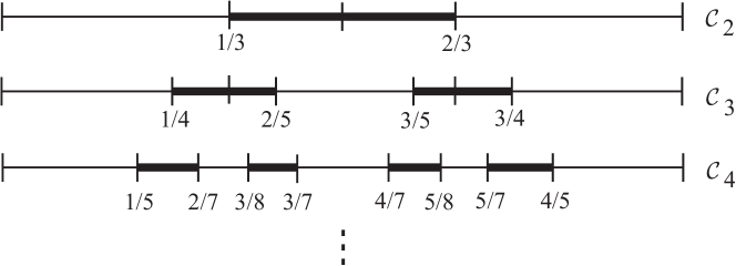
Figure 1. The first sum-level sets.

where we use the common notation $b_{n}\sim c_{n}$ to denote that $\lim_{n\to\infty}b_{n}/c_{n}=1$.

Theorem 1.2.

$$\sum_{k=1}^{n}\lambda\left(\mathcal{C}_{k}\right)\sim\frac{n}{\log_{2}n}.$$

Our third theorem gives a significant improvement of Theorem 1.1 and Theorem 1.2. That is, by increasing the dosage of infinite ergodic theory, we obtain the following sharp estimate for the asymptotic behaviour of the Lebesgue measure of the sum-level sets.

Theorem 1.3.

$$\lambda(\mathcal{C}_{n})\sim\frac{1}{\log_{2}n}.$$

We then continue by relating these results on the sum-level sets to the thermodynamical analysis of the Stern–Brocot system obtained in [17]. We obtain the, on a first sight, slightly surprising result that this thermodynamical analysis can be obtained from an exclusive use of either the sequence $\left(\mathcal{C}_{n}\right)$ or alternatively its complementary sequence $\left(\mathcal{C}_{n}^{c}\right)$, rather than using the Stern–Brocot sequence in total. In particular, this reveals that the vanishing of $\lim_{n\to\infty}\lambda(\mathcal{C}_{n})$ is very much a phenomenon of the fact that the Stern–Brocot system has a phase transition of order two at the point at which infinite ergodic theory takes over the regime from finite ergodic theory. A detailed discussion of this application to the thermodynamical formalism is given in Section 6. Finally, in Section 7, we apply Theorem 1.3 to classical metrical Diophantine analysis, and derive in this way a certain algebraic Khintchine-like law (see Lemma 7.1).

2. Sum-level sets, Stern–Brocot intervals, and the infinite Farey system

In the introduction we defined the sequence $\left(\mathcal{C}_{n}\right)$ of sum-level sets via the sum of the first entries in the continued fraction expansions. For later convenience, let us also add $\mathcal{C}_{0}:=[0,1]$ to this sequence. Let us begin with some brief comments on various equivalent ways of expressing the sum-level sets.

2.1. $\boldsymbol{\mathcal{C}_{n}}$ in terms of Stern–Brocot intervals

Recall the following classical construction of Stern–Brocot intervals (SB–intervals) (cf. [23], [4]). For each $n\in\mathbb{N}_{0}$, the elements of the $n$-th member of the Stern–Brocot sequence

$$\left\{\frac{s_{n,k}}{t_{n,k}}:k=1,\ldots,2^{n}+1\right\}$$

are defined recursively as follows:

• $s_{0,1}:=0\,\,$ and $\,\,s_{0,2}:=t_{0,1}:=t_{0,2}:=1$;

• $s_{n+1,2k-1}:=s_{n,k}\quad\textrm{and}\quad t_{n+1,2k-1}:=t_{n,k},$ for $k=1,\ldots,2^{n}+1$;

• $s_{n+1,2k}:=s_{n,k}+s_{n,k+1}\quad\textrm{and}\quad t_{n+1,2k}:=t_{n,k}+t_{n,k+1}$, for $k=1,\ldots 2^{n}$.

The set $\mathcal{T}_{n}$ of SB–intervals of order $n$ is given by

$$\mathcal{T}_{n}:=\left\{\left[\frac{s_{n,k}}{t_{n,k}},\frac{s_{n,k+1}}{t_{n,k+1}}\right]:\,k=1,\ldots,2^{n}\right\}.$$

By means of these intervals, the sum-level sets $\mathcal{C}_{n}$ are then given as follows. For $n=0,1$, we have $\mathcal{C}_{0}=[s_{0,1}/t_{0,1},s_{0,2}/t_{0,2}]$ and $\mathcal{C}_{1}=[s_{1,2}/t_{1,2},s_{1,3}/t_{1,3}]$. For $n>1$, we have

$$\mathcal{C}_{n}=\bigcup_{k=1}^{2^{n-2}}\left[\frac{s_{n,4k-2}}{t_{n,4k-2}},\frac{s_{n,4k}}{t_{n,4k}}\right].$$

Note that this point of view of $\mathcal{C}_{n}$ is the one chosen in [9], where $\mathcal{C}_{n}$ was referred to as the set of even intervals. Also, note that these even intervals are not SB–intervals. However, we clearly have that each of them is the union of two neighbouring SB–intervals of order $n$. That is,

$$\left[\frac{s_{n,4k-2}}{t_{n,4k-2}},\frac{s_{n,4k}}{t_{n,4k}}\right]=\left[\frac{s_{n,4k-2}}{t_{n,4k-2}},\frac{s_{n,4k-1}}{t_{n,4k-1}}\right]\cup\left[\frac{s_{n,4k-1}}{t_{n,4k-1}},\frac{s_{n,4k}}{t_{n,4k}}\right].$$

Throughout, we will use the notation $\mathcal{C}_{n}^{c}$ to denote the set of SB–intervals of order $n$ that are not in $\mathcal{C}_{n}$. Also, by slight abuse of notation, occasionally we will write $I\in\mathcal{C}_{n}$ for a SB–interval $I\in\mathcal{T}_{n}$ which is a subset of $\mathcal{C}_{n}$.

2.2. $\boldsymbol{\mathcal{C}_{n}}$ in terms of Stern–Brocot coding

There is also a way of expressing the sequence $\left(\mathcal{C}_{n}\right)$ in terms of the maps $\alpha,\beta:\mathcal{C}_{0}\to\mathcal{C}_{0}$ given by

$$\alpha(x):=x/(1+x)\mbox{ and }\beta\left(x\right):=1/(2-x).$$

It is well known that the orbit of the unit interval under the free semi-group generated by $\alpha$ and $\beta$ is in 1–1 correspondence to the set of SB-intervals. In fact, by associating the symbol $A$ to the map $\alpha$ and the symbol $B$ to the map $\beta,$ one obtains that each SB-interval (with the exception the SB-interval of order $0$) is associated with a unique word made of letters from the alphabet $\{A,B\},$ and vice versa. We will refer to this coding as the Stern–Brocot coding, and will write $I\cong W$ if $I$ is the SB-interval whose Stern–Brocot code is given by $W\in\{A,B\}^{k}$, for some $k\in\mathbb{N}$. The reader might like to recall that there is a dictionary which translates between Stern–Brocot intervals and continued fraction cylinder sets $[[a_{1},\ldots,a_{n}]]:=\{[x_{1},x_{2},\ldots]:x_{k}=a_{k},k=1,\ldots,n\}$, which reads as follows. For $\{X,Y\}=\{U,V\}=\{A,B\},$ we have

$$X^{a_{1}}Y^{a_{2}}X^{a_{3}}\cdots U^{a_{k}}V\cong\left\{\begin{array}[]{lll}[[a_{1}+1,a_{2},a_{3},\ldots,a_{k}]]&\,\,\textrm{for}&X=A\\ {}[[1,a_{1},a_{2},\ldots,a_{k}]]&\,\,\textrm{for}&X=B.\end{array}\right.$$

By using this dictionary, it is not hard to see that for $n\geq 2$ we have

$$\mathcal{C}_{n}=\{I\in\mathcal{T}_{n}:I\cong WXY\mbox{ for $\{X,Y\}=\{A,B\}$ and $W\in\{A,B\}^{n-2}$}\}.$$

To illustrate this way of viewing $\mathcal{C}_{n}$, we list the first members of this sequence of code words:

$$\mathcal{C}_{1}: B$$

$$\mathcal{C}_{2}: AB\,\,\,\,BA$$

$$\mathcal{C}_{3}: AAB\,\,\,\,ABA\,\,\,\,BAB\,\,\,\,BBA$$

$$\mathcal{C}_{4}: AAAB\,\,\,\,AABA\,\,\,\,ABAB\,\,\,\,ABBA\,\,\,\,BAAB\,\,\,\,BABA\,\,\,\,BBAB\,\,\,\,BBBA$$

$$\vdots$$

2.3. $\boldsymbol{\mathcal{C}_{n}}$ in terms of the Farey map

The sequence $\left(\mathcal{C}_{n}\right)$ can also be expressed with the help of the Farey map $T:\mathcal{C}_{0}\rightarrow\mathcal{C}_{0}$. For this, recall that $T$ is given by

$$T\left(x\right):=\left\{\begin{array}[]{lll}x/(1-x)&\,\,\textrm{for}&x\in\left[0,1/2\right]\\ (1-x)/x&\,\,\textrm{for}&x\in\left(1/2,1\right],\end{array}\right.$$

and that the inverse branches of $T$ are given by

$$u_{0}\left(x\right):=x/(1+x)\mbox{ and }u_{1}\left(x\right):=1/(1+x).$$

The associated Markov partition is then given by $\{L,R\}$, where $L:=\mathcal{C}_{0}\setminus\mathcal{C}_{1}$ and $R:=\mathcal{C}_{1}$, and each irrational number in $\mathcal{C}_{0}$ has a Markov coding $x=\langle x_{1},x_{2},\ldots\rangle\in\{L,R\}^{\mathbb{N}}$, given by $T^{k-1}(x)\in x_{k}$ for all $k\in\mathbb{N}$. This coding will be referred to as the Farey coding, and will write $I\triangleq W$ if $I$ is the SB-interval whose Farey code is given by $W\in\{L,R\}^{k}$, for some $k\in\mathbb{N}$. The dictionary which translates between Farey codes and continued fraction cylinders reads as follows:

$$L^{a_{1}-1}RL^{a_{2}-1}RL^{a_{3}-1}\cdots L^{a_{k}-1}R\triangleq[[a_{1},a_{2},a_{3},\ldots,a_{k}]].$$

By using this dictionary, it is not hard to see that we have, for each $n\in\mathbb{N}$,

$$\mathcal{C}_{n}=\{I\in\mathcal{T}_{n}:I\triangleq WR\mbox{ for $W\in\{L,R\}^{n-1}$}\}.$$

Again, let us list the first members of this sequence of code words:

$$\mathcal{C}_{1}: R$$

$$\mathcal{C}_{2}: LR\,\,\,\,RR$$

$$\mathcal{C}_{3}: LLR\,\,\,\,LRR\,\,\,\,RLR\,\,\,\,RRR$$

$$\mathcal{C}_{4}: LLLR\,\,\,\,LLRR\,\,\,\,LRRR\,\,\,\,LRLR\,\,\,\,RRLR\,\,\,\,RRRR\,\,\,\,RLRR\,\,\,\,RLLR$$

$$\vdots$$

The crucial link between the sequence of sum-level sets and the Farey map is now given by the following lemma.

Lemma 2.1.

For all $n\in\mathbb{N}$, we have that

$$T^{-(n-1)}(\mathcal{C}_{1})=\mathcal{C}_{n}.$$

Proof.

By computing the images of $\mathcal{C}_{1}$ under $u_{0}$ and $u_{1}$, one immediately verifies that $T^{-1}(\mathcal{C}_{1})=\mathcal{C}_{2}$. We then proceed by way of induction as follows. Assume that for some $n\in\mathbb{N}$ we have that $T^{-(n-1)}(\mathcal{C}_{1})=\mathcal{C}_{n}$. Since $T^{-n}(\mathcal{C}_{1})=T^{-1}(T^{-(n-1)}(\mathcal{C}_{1}))=T^{-1}(\mathcal{C}_{n})$, it is then sufficient to show that $T^{-1}(\mathcal{C}_{n})=\mathcal{C}_{n+1}$. For this, let $x=[a_{1},a_{2},\ldots]\in\mathcal{C}_{n}$ be given. Then there exists $\ell\in\mathbb{N}$ such that $x\in[[a_{1},\ldots,a_{\ell}]]$ and $\sum_{i=1}^{\ell}a_{i}=n$. By computing the images of $x$ under $u_{0}$ and $u_{1}$, one immediately obtains that $T^{-1}(x)=\{[1,a_{1},a_{2},\ldots],[a_{1}+1,a_{2},\ldots]\}$. Clearly, since $1+\sum_{i=1}^{\ell}a_{i}=(a_{1}+1)+\sum_{i=2}^{\ell}a_{i}=n+1$, this shows that $T^{-1}(x)\subset\mathcal{C}_{n+1}$, and hence, $T^{-1}(\mathcal{C}_{n})\subset\mathcal{C}_{n+1}$. The reverse inclusion $\mathcal{C}_{n+1}\subset T^{-1}(\mathcal{C}_{n})$ follows for instance by counting the SB–intervals in $\mathcal{C}_{n+1}$ and using the dictionary translating between SB–intervals and continued fraction cylinder sets. ∎

2.4. Elementary ergodic theory for the Farey map

For later use we now recall a few elementary facts and results from infinite ergodic theory for the Farey map. It is well known that the infinite Farey system $\left(\mathcal{C}_{0},T,\mathcal{A},\mu\right)$ is a conservative ergodic measure preserving dynamical system. Here, $\mathcal{A}$ refers to the Borel $\sigma$-algebra of $\mathcal{C}_{0}$, and the measure $\mu$ is the infinite $\sigma$-finite $T$-invariant measure absolutely continuous with respect to the Lebesgue measure $\lambda$. In fact, with $\varphi_{0}:\mathcal{C}_{0}\to\mathcal{C}_{0}$ defined by $\varphi_{0}(x):=x$, it is well known that $\mu$ is explicitly given by (see e.g. [6], [20] , [21])

$$\mathrm{d}\lambda=\varphi_{0}\,\mathrm{d}\mu.$$

Recall that conservative and ergodic means that $\sum_{n\geq 0}\widehat{T}^{n}\left(f\right)=\infty$, $\mu$-almost everywhere and for all $f\in L_{1}^{+}\left(\mu\right):=\left\{f\in L_{1}\left(\mu\right):\;f\geq 0\;\mathrm{and}\;\mu(f\cdot\mathbbm{1}_{\mathcal{C}_{0}})>0\right\}$. Here, $\mathbbm{1}_{\mathcal{C}_{0}}$ refers to the characteristic function of $\mathcal{C}_{0}$. Also, invariance of $\mu$ under $T$ means $\widehat{T}\left(\mathbbm{1}_{\mathcal{C}_{0}}\right)=\mathbbm{1}_{\mathcal{C}_{0}}$, where $\widehat{T}:L_{1}\left(\mu\right)\to L_{1}\left(\mu\right)$ denotes the transfer operator associated with the infinite dynamical Farey system, which is a positive linear operator, given by

$$\mu\left(\mathbbm{1}_{C}\cdot\widehat{T}\left(f\right)\right)=\mu\left(\mathbbm{1}_{T^{-1}\left(C\right)}\cdot f\right),\mbox{ for all }f\in L_{1}\left(\mu\right),C\in\mathcal{A}.$$

Finally, note that the Perron–Frobenius operator $\mathcal{L}:L_{1}\left(\mu\right)\to L_{1}\left(\mu\right)$ of the Farey system is given by

$$\mathcal{L}\left(f\right)=\left|u_{0}^{\prime}\right|\cdot(f\circ u_{0})+\left|u_{1}^{\prime}\right|\cdot(f\circ u_{1}),\mbox{ for all }f\in L_{1}\left(\mu\right).$$

One then immediately verifies that the two operators $\widehat{T}$ and $\mathcal{L}$ are related as follows:

$$\widehat{T}\left(f\right)=\varphi_{0}\cdot\mathcal{L}\left(f/\varphi_{0}\right),\mbox{ for all }f\in L_{1}\left(\mu\right).$$

Remark 2.2.

Let us remark that $\left(\mathcal{C}_{n}\right)$ has the following topological self-similarity property. Note that the set of SB–intervals of order $2$ consists of four SB–intervals, that is, a pair of adjacent intervals in the middle whose union is equal to $\mathcal{C}_{2}$, and two surrounding intervals, one to the left and the other to the right of this pair, where the union of the latter two is equal to $\mathcal{C}_{2}^{c}$. This structure of how the intervals of $\mathcal{C}_{2}$ and $\mathcal{C}_{2}^{c}$ appear in the set of SB–intervals of order $2$ serves as the building block for the topological structure of the appearance of the intervals in $\mathcal{C}_{n}\cup\mathcal{C}_{n}^{c}$ in general. Namely, for $n>2$, the set of SB–intervals of order $n$ consists of $2^{n}$ SB–intervals which are grouped into $2^{n-2}$ blocks of four adjacent intervals. The appearance of the intervals in each of these blocks looks topologically like a scaled down version of the building block at $n=2$ (see Figure 1). This point of view will be useful in the proof of Lemma 3.1 below, where we will employ a finite inductive process in order to locate a certain subset of $\mathcal{C}_{n}^{c}$.

3. Proof(s) of Theorem 1.1

In this section we give two alternative proofs of Theorem 1.1. The first of these is more elementary, whereas the second uses exactness of $T$ and a criterion for exactness due to Lin.

3.1. First Proof of Theorem 1.1

The following lemma gives the first step in our first proof of Theorem 1.1. Note that the statement of this lemma has already been obtained in [9], where it was the main result. Nevertheless, in order to keep the paper as self-contained as possible, we give a short proof of this result.

Lemma 3.1.

$$\liminf_{n\to\infty}\,\lambda(\mathcal{C}_{n})=0.$$

Proof.

Let $n\in\mathbb{N}$ be fixed such that $n>3$, and let $k\in\{2,\ldots,n-2\}$ be arbitrary. Recall that the set of SB–intervals of order $k$ consists of $2^{k-2}$ blocks of four adjacent SB–intervals (see Remark 2.2). Now, let $I\subset{\mathcal{C}}_{k}$ be a SB–interval of order $k$ such that $I\cong W\in\{A,B\}^{k}$. We then have that $I$ contains the interval $I_{A,n-k}\cong WA^{n-k}$ as well as the interval $I_{B,n-k}\cong WB^{n-k}$. Note that $I_{A,n-k}$ and $I_{B,n-k}$ are two distinct SB–intervals of order $n$ which are both contained in ${\mathcal{C}}_{n}^{c}$. Also, it is well known (see e.g. [16]) that in this situation we have, where $a_{n}\asymp b_{n}$ means that the quotient $a_{n}/b_{n}$ is uniformly bounded away from zero and infinity,

$$\lambda(I)\asymp(n-k)\lambda(I_{X,n-k}),\mbox{ for each }X\in\{A,B\}.$$

Clearly, $I_{X,n-k}\cap J_{Y,n-k}=\emptyset$, for all $X\in\{A,B\}$, $I,J\in{\mathcal{C}}_{k}$ ($I\neq J$). Moreover, by construction, we have for each $k,l\in\{2,\ldots,n-2\}$ such that $k\neq l$ and such that either $k$ and $l$ are both odd or both even,

$$I_{X,n-k}\cap J_{Y,n-l}=\emptyset,\mbox{ for all }I\in{\mathcal{C}}_{k},J\in{\mathcal{C}}_{l},X\in\{A,B\}.$$

Note that in here we require that $k$ and $l$ are both odd or both even, since for instance for the interval $I\in{\mathcal{C}}_{2}$ for which $I\cong AB$ and the interval $J\in{\mathcal{C}}_{3}$ for which $J\cong ABA$ we have that $I_{A,n-2}=J_{A,n-3}$. Also, note that we require $k<n-1$, since for instance for the interval $I\in{\mathcal{C}}_{n-1}$ for which $I\cong WB$ we have that $I_{A,1}\notin{\mathcal{C}}_{n}^{c}$. It now follows that for each $k<n-1$ we have

$$\frac{1}{n-k}\lambda(\mathcal{C}_{k})=\sum_{I\in{\mathcal{C}}_{k}}\frac{1}{n-k}\lambda(I)\asymp\sum_{I\in{\mathcal{C}}_{k}}\sum_{X\in\{A,B\}}\lambda(I_{X,n-k}).$$

Combining these observations, we obtain that

$$\sum_{{k=2}}^{n-2}\frac{1}{n-k}\lambda(\mathcal{C}_{k})\asymp\sum_{k=2}^{n-2}\sum_{I\in{\mathcal{C}}_{k}}\sum_{X\in\{A,B\}}\lambda(I_{X,n-k})\leq 2\lambda(\mathcal{C}_{n}^{c}).$$

To finish the proof, let us assume by way of contradiction that $\liminf_{n\to\infty}\lambda(\mathcal{C}_{n})=\kappa>0$. By the above, we then have that

$$1\geq\lambda(\mathcal{C}_{n}^{c})\gg\sum_{{k=2}}^{n-2}\frac{1}{n-k}\lambda(\mathcal{C}_{k})\gg\kappa\sum_{{k=2}}^{n-1}\frac{1}{k}\gg\log n,\mbox{ for all }n\in\mathbb{N},$$

where $a_{n}\gg b_{n}$ means that the quotient $a_{n}/b_{n}$ is uniformly bounded away from zero. This gives a contradiction, and hence finishes the proof. ∎

For the first proof of Theorem 1.1 we also require the following lemma. For this, the reader might like to recall from Section 2 that the function $\varphi_{0}:\mathcal{C}_{0}\to\mathcal{C}_{0}$ is given by $\varphi_{0}(x):=x$.

Lemma 3.2.

On $\mathcal{C}_{1}$ we have

$$\widehat{T}^{n}\varphi_{0}<\widehat{T}^{n-1}\varphi_{0},\mbox{ {\it for all} }n\in\mathbb{N}.$$

Proof.

Recall that $\widehat{T}g=\varphi_{0}\cdot\mathcal{L}(g/\varphi_{0})$, where $\mathcal{L}(g)=\sum_{i=0}^{1}\left(\left|(T^{-1})^{\prime}\right|\cdot(g\circ u_{i})\right)$, that is,

$$\widehat{T}g\left(x\right)=\frac{g\left(u_{0}(x)\right)+x\cdot g\left(u_{1}(x)\right)}{1+x}.$$

By [13, Lemma 3.2] it follows that for $\mathcal{D}:=\left\{g\in C^{2}\left(\left[0,1\right]\right):g^{\prime}\geq 0,g^{\prime\prime}\leq 0\>\right\}$ we have $\widehat{T}\left(\mathcal{D}\right)\subset\mathcal{D}$. The latter displayed formula in particular also shows that $f\left(1/2\right)=\widehat{T}f(1)$. Moreover, one immediately verifies that $\varphi_{0}\in\mathcal{D}$. Hence, for all $x\in\mathcal{C}_{1}$ we have

$$\widehat{T}^{n}\varphi_{0}(x) \leq \max\left\{\widehat{T}^{n}\varphi_{0}(x):x\in\mathcal{C}_{1}\right\}=\widehat{T}^{n}\varphi_{0}(1)=\widehat{T}^{n-1}\varphi_{0}\left(1/2\right)$$

$$= \min\left\{\widehat{T}^{n-1}\varphi_{0}(x):x\in\mathcal{C}_{1}\right\}\leq\widehat{T}^{n-1}\varphi_{0}\left(x\right).$$

∎

First proof of Theorem 1.1.

Using Lemma 2.1, Lemma 3.2, the $T$-invariance of $\mu$, and the fact that $\mathrm{d}\lambda=\varphi_{0}\cdot\mathrm{d}\mu$, we obtain

$$\lambda(\mathcal{C}_{n+1}) = \mu\left(\mathbbm{1}_{\mathcal{C}_{n+1}}\cdot\varphi_{0}\right)=\mu\left(\mathbbm{1}_{T^{-n}(\mathcal{C}_{1})}\cdot\varphi_{0}\right)=\mu\left(\mathbbm{1}_{\mathcal{C}_{1}}\cdot\widehat{T}^{n}(\varphi_{0})\right)$$

$$< \mu\left(\mathbbm{1}_{\mathcal{C}_{1}}\cdot\widehat{T}^{n-1}(\varphi_{0})\right)=\mu\left(\mathbbm{1}_{\mathcal{C}_{n}}\cdot\varphi_{0}\right)=\lambda(\mathcal{C}_{n}).$$

Hence, the sequence $\left(\lambda(\mathcal{C}_{n})\right)$ is strictly decreasing. Combining this fact with Lemma 3.1, our first proof of Theorem 1.1 is complete. ∎

3.2. Second Proof of Theorem 1.1

For the second proof of Theorem 1.1 recall that a non-singular transformation $S$ of the $\sigma$–finite measure space $\left(\mathcal{C}_{0},\mathcal{A},m\right)$ is called exact if and only if for each element $A$ of the tail $\sigma$-algebra $\bigcap_{n\in\mathbb{N}}S^{-n}\left(\mathcal{A}\right)$ we have that $m(A)\cdot m(A^{c})=0$. Crucial for us here will be a result of Lin [19] which gives a necessary and sufficient condition for exactness of $S$ in terms the dual $\widehat{S}$ of $S$. More precisely, Lin found that $S$ is exact if and only if

$$\lim_{n\to\infty}\|\widehat{S}^{n}(f)\|_{1}=0,\mbox{ for all $f\in L_{1}(m)$ such that $m(f)=0$}.$$

We begin with by showing that the infinite Farey system $\left(\mathcal{C}_{0},T,\mathcal{A},\mu\right)$ is exact. Let us remark that this fact is probably well known to experts in the field of infinite ergodic theory of numbers. Nevertheless, we were unable to locate a rigorous proof in the literature, and hence decided to give such a proof here. However, our proof was inspired by the proof of [2, Theorem 3.2].

Proposition 3.3.

The Farey map $T$ of the $\sigma$–finite measure space $\left(\mathcal{C}_{0},\mathcal{A},\mu\right)$ is exact.

Proof.

Let $A_{0}\in\bigcap_{n\in\mathbb{N}}T^{-n}\mathcal{A}$ be given such that $m_{{\mathfrak{g}}}(A_{0})>0$, where $dm_{{\mathfrak{g}}}(x)=(\log(2)(1+x))^{-1}d\lambda(x)$ denotes the Gauss measure. Note that, since $\mu$ and $m_{{\mathfrak{g}}}$ are in the same measure class, it is sufficient to show the exactness of $T$ with respect to $m_{{\mathfrak{g}}}$, rather than $\mu$. Therefore, the aim is to show that $m_{{\mathfrak{g}}}(A_{0}^{c})=0$. For this, first note that, since $A_{0}\in\bigcap_{n\in\mathbb{N}}T^{-n}\mathcal{A}$, there exists a sequence $\left(A_{n}\right)_{n\in\mathbb{N}}$ such that $A_{n}\in\mathcal{A}$ and $A_{0}=T^{-n}A_{n}$, for all $n\in\mathbb{N}$. Clearly, we then have that $A_{k+m}=T^{k}A_{m}$, for all $k,m\in\mathbb{N}_{0}$. For each $x\in\mathcal{C}_{0}$, let $\rho$ be defined by

$$\rho(x):=\inf\left\{n\geq 0:T^{n}\left(x\right)\in\mathcal{C}_{1}\right\}.$$

Since $T$ is conservative, we have that $\rho$ is finite, $m_{{\mathfrak{g}}}$-almost everywhere. Define $\rho_{n}:=\sum_{k=0}^{n-1}\rho\circ\left(\mathfrak{g}^{k}\right)$, and let $\langle\langle x_{1},\ldots,x_{n}\rangle\rangle:=\{\langle y_{1},y_{2},\ldots\rangle:y_{k}=x_{k},k=1,\ldots,n\}$ denote a cylinder set arising from the Farey coding. Using the facts that $m_{{\mathfrak{g}}}$ is $\mathfrak{g}$–invariant and of bounded mixing type with respect to ${\mathfrak{g}}$, we obtain for $m_{{\mathfrak{g}}}$–almost every $x=\langle x_{1},x_{2},\ldots\rangle=[a_{1},a_{2},\ldots]$,

$$m_{{\mathfrak{g}}}\left(A_{0}|\langle\langle x_{1},\ldots,x_{\rho_{n}\left(x\right)+1}\rangle\rangle\right) = \frac{m_{{\mathfrak{g}}}\left(A_{0}\cap\langle\langle x_{1},\ldots,x_{\rho_{n}\left(x\right)+1}\rangle\rangle\right)}{m_{{\mathfrak{g}}}\left(\langle\langle x_{1},\ldots,x_{\rho_{n}\left(x\right)+1}\rangle\rangle\right)}$$

$$= \frac{m_{{\mathfrak{g}}}\left(T^{-(\rho_{n}\left(x\right)+1)}A_{\rho_{n}\left(x\right)+1}\cap\langle\langle x_{1},\ldots,x_{\rho_{n}\left(x\right)+1}\rangle\rangle\right)}{m_{{\mathfrak{g}}}\left(\langle\langle x_{1},\ldots,x_{\rho_{n}\left(x\right)+1}\rangle\rangle\right)}$$

$$= \frac{m_{{\mathfrak{g}}}\left({\mathfrak{g}}^{-n}A_{\rho_{n}\left(x\right)+1}\cap\langle\langle x_{1},\ldots,x_{\rho_{n}\left(x\right)+1}\rangle\rangle\right)}{m_{{\mathfrak{g}}}\left(\langle\langle x_{1},\ldots,x_{\rho_{n}\left(x\right)+1}\rangle\rangle\right)}$$

$$= \frac{m_{{\mathfrak{g}}}\left({\mathfrak{g}}^{-n}A_{\rho_{n}\left(x\right)+1}\cap[[a_{1},\ldots,a_{n}]]\right)}{m_{{\mathfrak{g}}}\left([[a_{1},\ldots,a_{n}]]\right)}$$

$$\asymp \frac{m_{{\mathfrak{g}}}\left({\mathfrak{g}}^{-n}A_{\rho_{n}\left(x\right)+1}\right)m_{{\mathfrak{g}}}\left([[a_{1},\ldots,a_{n}]]\right)}{m_{{\mathfrak{g}}}\left([[a_{1},\ldots,a_{n}]]\right)}={m_{{\mathfrak{g}}}\left(A_{\rho_{n}\left(x\right)+1}\right)}.$$

Also, by the Martingale Convergence Theorem (cf. [7]), we have for $m_{{\mathfrak{g}}}$-almost every $x=\langle x_{1},x_{2},\ldots\rangle$,

$$\lim_{n\to\infty}m_{{\mathfrak{g}}}\left(A_{0}|\langle\langle x_{1},\ldots,x_{\rho_{n}\left(x\right)+1}\rangle\rangle\right)=\mathbbm{1}_{A_{0}}(x).$$

Combining the two latter observations, it follows that $A_{0}=\Lambda\mod m_{\mathfrak{g}}$, where $\Lambda$ is defined by

$$\Lambda:=\{x\in\mathcal{C}_{0}:\liminf_{n}{m_{{\mathfrak{g}}}\left(A_{\rho_{n}\left(x\right)+1}\right)}>0\}.$$

Since, by assumption, $m_{{\mathfrak{g}}}(A_{0})>0$, we now have that $m_{{\mathfrak{g}}}(\Lambda)>0$. Hence, to finish the proof, we are left to show that $m_{{\mathfrak{g}}}(\Lambda)=1$. For this recall that $m_{{\mathfrak{g}}}$ is ergodic and $\mathfrak{g}$–invariant. This gives that it is in fact sufficient to show that ${\mathfrak{g}}^{-1}\Lambda\subset\Lambda\mod m_{{\mathfrak{g}}}$. In other words, in order to complete the proof, we are left to show that $\liminf_{n}m_{{\mathfrak{g}}}(A_{\rho_{n}({\mathfrak{g}}(x))+1})>0$ implies $\liminf_{n}m_{{\mathfrak{g}}}(A_{\rho_{n}(x)+1})>0$. Since $A_{\rho_{n+1}(x)+1}=A_{\rho(x)+\rho_{n}({\mathfrak{g}}(x))+1}=T^{\rho(x)}A_{\rho_{n}({\mathfrak{g}}(x))+1}$, this assertion would follow if we establish that for each $\varepsilon>0$ and $\ell\in\mathbb{N}$ there exists $\kappa>0$ such that for all $B\in\mathcal{A}$ with $m_{{\mathfrak{g}}}(B)>\varepsilon$ we have $m_{{\mathfrak{g}}}(T^{\ell}B)>\kappa$. Hence, let us assume that $m_{{\mathfrak{g}}}(B)>\varepsilon$, and let $\alpha_{\ell}$ denote the Markov partition for the map $T^{\ell}$. Clearly, there are $2^{\ell}$ elements in $\alpha_{\ell}$. This immediately implies that $m_{{\mathfrak{g}}}(A\cap B)>\varepsilon 2^{-\ell}$, for some $A\in\alpha_{\ell}$. Therefore, using the fact that $T^{\ell}:A\to\mathcal{C}_{0}$ is bijective and the fact that there exists a constant $c_{0}>0$ such that $dm_{{\mathfrak{g}}}\circ T^{\ell}/dm_{{\mathfrak{g}}}(y)>c_{0}$ for all $y\in A$, it follows that $m_{{\mathfrak{g}}}(T^{\ell}B)>c_{0}2^{-\ell}\varepsilon$. Hence, by setting in the above $\kappa:=c_{0}2^{-\ell}\varepsilon$, the proof follows. ∎

Proposition 3.4.

For each $C\in\mathcal{A}$ with $\mu\left(C\right)<\infty$, we have that

$$\lim_{n\to\infty}\lambda\left(T^{-n}(C)\right)=0.$$

Proof.

Let $C\in\mathcal{A}$ be given as stated in the proposition. For each $A\in\mathcal{A}$ for which $0<\mu\left(A\right)<\infty$, we then have

$$\lambda\left(T^{-n}(C)\right) = \mu\left(\mathbf{1}_{T^{-n}(C)}\,\cdot\varphi_{0}\right)=\mu\left(\mathbf{1}_{C}\circ T^{n}\cdot\varphi_{0}\right)$$

$$= \mu\left(\mathbf{1}_{C}\circ T^{n}\cdot\left(\varphi_{0}-\frac{\mathbf{1}_{A}}{\mu\left(A\right)}+\frac{\mathbf{1}_{A}}{\mu\left(A\right)}\right)\right)$$

$$\leq \left\|\widehat{T}^{n}\left(\varphi_{0}-\frac{\mathbf{1}_{A}}{\mu\left(A\right)}\right)\right\|_{1}+\frac{\mu\left(T^{-n}\left(C\right)\cap A\right)}{\mu\left(A\right)}$$

$$\leq \left\|\widehat{T}^{n}\left(\varphi_{0}-\frac{\mathbf{1}_{A}}{\mu\left(A\right)}\right)\right\|_{1}+\frac{\mu\left(C\right)}{\mu\left(A\right)}\longrightarrow\frac{\mu\left(C\right)}{\mu\left(A\right)},\mbox{ for $n$ tending to infinity}.$$

Here, the latter follows, since $T$ is exact and $\mu\left(\left(\varphi_{0}-{\mathbbm{1}}_{A}/\mu\left(A\right)\right)\right)=0$, and hence, Lin’s criterion, mentioned at the beginning of this section, is applicable. Therefore, by choosing $\mu\left(A\right)$ arbitrarily large, the proposition follows. ∎

Second proof of Theorem 1.1.

In Proposition 3.4 put $C=\mathcal{C}_{1}$, and then use the fact that $\mathcal{C}_{n}=T^{-(n-1)}(\mathcal{C}_{1})$, for all $n\in\mathbb{N}$. ∎

4. Proof of Theorem 1.2

Proof.

We employ several standard arguments from infinite ergodic theory. First, note that it is well known that the induced map $T_{\mathcal{C}_{1}}$ of the Farey map $T$ on $\mathcal{C}_{1}$ is conjugate to the Gauss map $\mathfrak{g}$. This then immediately gives that $T_{\mathcal{C}_{1}}$ is continued fraction mixing (see [27]). Therefore, by [1, Lemma 3.7.4], it follows that $\mathcal{C}_{1}$ is a Darling–Kac set for $T$. This implies that there exists a sequence $\left(\nu_{n}\right)$ (the return sequence of $T$) such that

$$\lim_{n\to\infty}\frac{1}{\nu_{n}}\sum_{i=0}^{n-1}\widehat{T}^{i}\mathbbm{1}_{\mathcal{C}_{1}}(x)=\mu(\mathcal{C}_{1})=\log 2,\mbox{ uniformly for $\mu$-almost every }x\in\mathcal{C}_{1}.$$

In order to determine the asymptotic type of the sequence $(\nu_{n})$, recall from [1, Section 3.8] that for a set $C\in\mathcal{A}$ such that $0<\mu\left(C\right)<\infty$, the wandering rate of $C$ is given by the sequence $\left(W_{n}\left(C\right)\right)$, where

$$W_{n}\left(C\right):=\mu\left(\bigcup_{k=1}^{n}T^{-(k-1)}(C)\right).$$

Let us compute $\left(W_{n}(C)\right)$ for $C=\mathcal{C}_{1}$. Namely, for all $n\in\mathbb{N}$ we have

$$W_{n}\left(\mathcal{C}_{1}\right)=\mu\left(\bigcup_{k=1}^{n}T^{-(k-1)}\left(\mathcal{C}_{1}\right)\right)=\mu\left(\mathbbm{1}_{[1/(n+1),1]}\right)=\log(n+1).$$

Note that this wandering rate is slowly varying at infinity, that is (see e.g. [3]),

$$\lim_{n\to\infty}W_{k\cdot n}\left(\mathcal{C}_{1}\right)/W_{n}\left(\mathcal{C}_{1}\right)=1,\mbox{ for each }k\in\mathbb{N}.$$

Also, note that, since $T$ has a Darling–Kac set, it follows from [1, Proposition 3.7.5] that $T$ is pointwise dual ergodic with respect to $\mu$, that is,

$$\lim_{n\to\infty}\frac{1}{\nu_{n}}\sum_{i=0}^{n-1}\widehat{T}^{i}f=\mu(f),\mbox{ for all }f\in L^{1}(\mu).$$

In this situation we then have, by [1, Proposition 3.8.7], that the return sequence and the wandering rate are related through

$$\lim_{n\to\infty}(n\cdot v_{n}/W_{n}(\mathcal{C}_{1}))=1.$$

Combining these observations, the proof of Theorem 1.2 follows. ∎

Remark 4.1.

Although we are not going to use these facts here, let us nevertheless remark that the Farey map $T$ has the the following additional infinite ergodic theoretical properties. The verification of these properties follows from standard infinite ergodic theory (cf. [1], [2], [26]).

• The map $T$ is rationally ergodic with respect to $\mu$. That is, there exists a constant $c>0$ and a set $A$ with $0<\mu(A)<\infty$ such that for all $n\in\mathbb{N}$,

  $\displaystyle\int_{A}\bigg{(}\sum_{i=0}^{n-1}\mathbbm{1}_{A}\circ T^{i}\bigg{)}^{2}d\mu<c\,\bigg{(}\int_{A}\sum_{i=0}^{n-1}\mathbbm{1}_{A}\circ T^{i}d\mu\bigg{)}^{2}.$ $(\ast)$

• The map $T$ has the following mixing property. For $A$ with $0<\mu(A)<\infty$ such that $(\ast)$ holds, we have for all $U,V\subset A$,

  $$\lim_{n\to\infty}\frac{1}{\nu_{n}}\sum_{i=0}^{n-1}\mu(U\cap T^{-i}V)=\mu(U)\mu(V).$$

5. Proof of Theorem 1.3

Proof.

As already mentioned in the introduction, the proof of Theorem 1.3 will make use of some further, slightly more advanced infinite ergodic theory. Let us begin with by first giving the concepts and results which are relevant for the proof of Theorem 1.3. The following concept of a uniform set is vital in many situations within infinite ergodic theory, and this is also the case in our situation here. (For further examples of interval maps (including the Farey map) for which there exist uniform sets we refer to [24, 25].)

• ([1, Section 3.8]) A set $C\in\mathcal{A}$ with $0<\mu\left(C\right)<\infty$ is called uniform for $f\in L_{1}^{+}\left(\mu\right)$, if $\mu$–almost everywhere and uniformly on $C$ we have that

  $$\lim_{n\to\infty}\frac{1}{v_{n}}\sum_{k=0}^{n-1}\widehat{T}^{k}\left(f\right)=\mu(f),$$

  where $\left(v_{n}\right)$ denotes the return sequence of $T$, and uniform convergence is meant with respect to $L_{\infty}\left(\mu|_{C}\right)$.

Note that it is not difficult to see that the Farey map $T$ satisfies Thaler’s conditions, among which Adler’s condition, i.e. $T^{\prime\prime}/(T^{\prime})^{2}$ is bounded throughout $(0,1)$, is the most important one (see [24, 25]). This then immediately implies that we have the following, where, as in Section 2, the function $\varphi_{0}$ is given by $\varphi_{0}(x)=x$.

• Let $C\in\mathcal{A}$ be given with $\lambda\left(C\right)>0$ and so that there exists an $\varepsilon>0$ such that $x>\varepsilon$, for all $x\in C$. We then have that $C$ is a uniform set for the function $\varphi_{0}$.

Now, the crucial notion for proving the sharp asymptotic result of Theorem 1.3 is provided by the following concept of a uniformly returning set. (For further examples of one dimensional dynamical systems which allow uniformly returning sets for some appropriate function we refer to [26].)

• ([12]) A set $C\in\mathcal{A}$ with $0<\mu\left(C\right)<\infty$ is called uniformly returning for $f\in L_{\mu}^{+}$ if there exists a positive increasing sequence $\left(w_{n}\right)=\left(w_{n}(f,C)\right)$ of positive reals such that $\mu$–almost everywhere and uniformly on $C$ we have

  $$\lim_{n\to\infty}w_{n}\widehat{T}^{n}\left(f\right)=\mu(f).$$

In order to determine the asymptotic type of the sequence $\left(w_{n}\right)$, we use [12, Proposition 1.2] where we found that

$$\lim_{n\to\infty}W_{n}\left(C\right)/w_{n}=1,\mbox{ for all $C\in\mathcal{A}$ such that $0<\mu\left(C\right)<\infty$},$$

where $\left(W_{n}\left(C\right)\right)$ denotes the wandering rate, which we already considered in the proof of Theorem 1.2. In [12, Proposition 1.1] it was shown that every uniformly returning set is uniform. Whereas, in [13] we found explicit conditions under which also the reverse of this implication holds. Applying these results of [13] to our situation here, one obtains the following.

• ([13]) Let $C\in\mathcal{A}$ with $0<\mu\left(C\right)<\infty$ be a uniform set, for some $f\in L_{\mu}^{+}$. If the wandering rate $\left(W_{n}(C)\right)$ is slowly varying at infinity and if the sequence $\left(\widehat{T}^{n}\left(f\right)\mid_{C}\right)$ is decreasing, then we have that $C$ is a uniformly returning set for $f$. Moreover, $\mu$–almost everywhere and uniformly on $C$ we have

  $$\lim_{n\to\infty}W_{n}(C)\,\widehat{T}^{n}\left(f\right)=\mu(f).$$

With these preparations, we can now finish the proof of Theorem 1.3 as follows. The idea is to apply the results stated above to the situation in which the set $C$ is equal to $\mathcal{C}_{1}$. For this, first recall that we have already seen that the wandering rate $\left(W_{n}(\mathcal{C}_{1})\right)$ of $\mathcal{C}_{1}$ is obviously slowly varying at infinity. In fact, as computed in the proof of Theorem 1.2, we have that $\lim_{n\to\infty}n\cdot v_{n}/W_{n}(\mathcal{C}_{1})=1$, and also that $W_{n}(\mathcal{C}_{1})\sim\log n$. Secondly, since $\mathcal{C}_{1}$ is bounded away from zero, the result in (II) gives that $\mathcal{C}_{1}$ is a uniform set for $\varphi_{0}$. Thirdly, by Lemma 3.2, we have that the sequence $\big{(}\widehat{T}^{n}\left(\varphi_{0}\right)\mid_{\mathcal{C}_{1}}\big{)}$ is decreasing. Thus, we can apply the result in the first part of (IV), which then shows that $\mathcal{C}_{1}$ is a uniformly returning set for the function $\varphi_{0}$. Hence, the second part in (IV) gives that $\mu$–almost everywhere and uniformly on $\mathcal{C}_{1}$ we have

$$\lim_{n\to\infty}W_{n}(\mathcal{C}_{1})\,\widehat{T}^{n}\left(\varphi_{0}\right)=\mu(\varphi_{0})=1.$$

Combining these observations, it now follows that

$$\lim_{n\to\infty}\left(\log n\cdot\lambda\left(\mathcal{C}_{n}\right)\right)=\lim_{n\to\infty}\left(W_{n}(\mathcal{C}_{1})\cdot\mu\left(\mathbbm{1}_{\mathcal{C}_{1}}\cdot\widehat{T}^{n-1}(\varphi_{0})\right)\right)=\mu\left(\mathbbm{1}_{\mathcal{C}_{1}}\right)=\log 2.$$

This finishes the proof of Theorem 1.3. ∎

6. Thermodynamical significance of the sum-level sets

In this section we discuss the thermodynamical significance of the results of the previous sections. For this, recall that in [15] and [17] (see also [16]) we studied the multifractal spectrum $\{\tau(s):s\in\mathbb{R}\}$, given by

$$\tau(s):=\dim_{H}\left(\left\{x=[a_{1},a_{2},\ldots]:\lim_{n\rightarrow\infty}\frac{2\log q_{n}(x)}{\sum_{i=1}^{n}a_{i}}=s\right\}\right).$$

Here, $p_{n}(x)/q_{n}(x):=[a_{1},a_{2},\ldots,a_{n}]$ denotes the $n$-th approximant of $x$, and $\dim_{H}$ refers to the Hausdorff dimension. In order to compute this spectrum, the Stern–Brocot pressure function $P$ turns out to be crucial. This pressure function is defined for $t\in\mathbb{R}$ by

$$P(t):=\lim_{n\rightarrow\infty}\frac{1}{n}\log\sum_{I\in\mathcal{T}_{n}}\left(\mathop{\hbox{\rm diam}}(I)\right)^{t}.$$

The following results give the main outcome concerning the properties of $P$ and $\tau$ and on how these functions are related. This complete thermodynamical description of the Stern–Brocot system was obtained in [17, Theorem 1.1]. Here, $\gamma:=(1+\sqrt{5})/2$ denotes the Golden Mean, and $P^{*}$ refers to the Legendre transform of $P$, given for $s\in\mathbb{R}$ by $P^{*}(s):=\sup_{t\in\mathbb{R}}\{t\cdot s-P(t)\}$.

1. [17, Theorem 1.1]. For each $s\in[0,2\log\gamma]$, we have that

   $$\tau(s)=-P^{*}(-s)/s,$$

   with the convention that $\tau(0):=\lim_{s\searrow 0}-P^{*}(-s)/s=1$. Also, the dimension function $\tau$ is continuous and strictly decreasing on $[0,2\log\gamma]$ and vanishes outside the interval $[0,2\log\gamma)$. Moreover, the left derivative of $\tau$ at $2\log\gamma$ is equal to $-\infty$. The function $P$ is convex, non-increasing and differentiable throughout $\mathbb{R}$. Furthermore, $P$ is real-analytic on $(-\infty,1)$ and vanishes on $[1,\infty)$.

2. [11, 22] We have that

   $$P(1-\varepsilon)\sim-\varepsilon/\log\varepsilon,\mbox{ for $\varepsilon$ tending to zero form above}.$$

   In particular, the Farey system has a second order phase transition at $t=1$, that is, the function $P^{\prime}$ is continuous and $P^{\prime\prime}$ is discontinuous at $t=1$.

The following shows that the vanishing of $\lim_{n\to\infty}\lambda(\mathcal{C}_{n})$ is very much a phenomenon of the fact that the Stern–Brocot system exhibits a phase transition of order two at $t=1$. At this point of intermittency, finite ergodicity breaks down and infinite ergodic theory enters the scene. In particular, by (2), this abrupt transition from finite to infinite ergodic theory happens in a way which is non-smooth.

One aspect of this intermittency is given by the following. For this, recall that in [15, Proposition 2.6] it was also shown that for each $s\in(0,2\log\gamma]$ there exists an equilibrium measure $\nu_{s}$ for which $\dim_{H}(\nu_{s})=\tau(s)$. Using the invariance of $\nu_{s}$, one immediately verifies that for each $s\in(0,2\log\gamma]$ we have that

$$\nu_{s}(\mathcal{C}_{1})=\nu_{s}(\mathcal{C}_{n})=\nu_{s}(\mathcal{C}_{n}^{c})=1/2,\mbox{ for all }n\in\mathbb{N}.$$

In contrast to this, we have by Theorem 1.1 and Theorem 1.3 respectively,

$$\lim_{n\rightarrow\infty}\lambda(\mathcal{C}_{n})=0\mbox{ and }\lim_{n\rightarrow\infty}\lambda(\mathcal{C}_{n}^{c})=1.$$

Another aspect is provided by the following proposition, in which $P_{0}$ and $P_{1}$ denote the two partial Stern–Brocot pressure functions, given for $t\in\mathbb{R}$ by

$$P_{0}(t):=\lim_{n\rightarrow\infty}\frac{1}{n}\log\sum_{I\in\mathcal{C}_{n}}\left(\mathop{\hbox{\rm diam}}(I)\right)^{t}\mbox{ and }P_{1}(t):=\lim_{n\rightarrow\infty}\frac{1}{n}\log\sum_{I\in\mathcal{C}_{n}^{c}}\left(\mathop{\hbox{\rm diam}}(I)\right)^{t}.$$

Proposition 6.1.

The outcome of the above complete thermodynamical description of the Stern–Brocot system stays to be the same if we base the analysis exclusively on either $\{I\in\mathcal{C}_{n}:n\in\mathbb{N}\}$ or $\{I\in\mathcal{C}_{n}^{c}:n\in\mathbb{N}\}$, rather than on all the intervals in $\{I\in\mathcal{T}_{n}:n\in\mathbb{N}\}$. In particular, we have that

$$P(t)=P_{0}(t)=P_{1}(t),\mbox{ for all }t\in\mathbb{R}.$$

Proof.

Using the recursive definition of the Stern–Brocot sequence, one immediately verifies that

$$t_{n-1,2k-1}\,t_{n-1,2k}\leq t_{n,4k-2}\,t_{n,4k-1}\leq n\,\,t_{n-1,2k-1}\,t_{n-1,2k},$$

and

$$t_{n-1,2k}\,t_{n-1,2k+1}\leq t_{n,4k-1}\,t_{n,4k}\leq n\,\,t_{n-1,2k}\,t_{n-1,2k+1}.$$

Combining these observations, we obtain

$$n^{-|t|}\,\sum_{I\in\mathcal{T}_{n-1}}\left(\mathop{\hbox{\rm diam}}(I)\right)^{t}\leq\sum_{I\in\mathcal{C}_{n}}\left(\mathop{\hbox{\rm diam}}(I)\right)^{t}\leq n^{|t|}\,\sum_{I\in\mathcal{T}_{n-1}}\left(\mathop{\hbox{\rm diam}}(I)\right)^{t}.$$

This shows that $P(t)=P_{0}(t)$, for all $t\in\mathbb{R}$. The proof of $P(t)=P_{1}(t)$ follows by similar means, and is left to the reader. ∎

Remark 6.2.

Note that Feigenbaum, Procaccia and Tél [8] explored what they called the Farey tree model. This model is based on the set of even intervals

$$\left\{\left[\frac{s_{n,4k-2}}{t_{n,4k-2}},\frac{s_{n,4k}}{t_{n,4k}}\right]:k=1,\ldots,2^{n-2}\right\},\mbox{ for all }n\in\mathbb{N}.$$

Note that for the even intervals of any order $n\in\mathbb{N}$ we have, for all $t\in\mathbb{R}$,

$$\left(\mathop{\hbox{\rm diam}}\left(\left[\frac{s_{n,4k-2}}{t_{n,4k-2}},\frac{s_{n,4k}}{t_{n,4k}}\right]\right)\right)^{t}$$

$$= \left(\mathop{\hbox{\rm diam}}\left(\left[\frac{s_{n,4k-2}}{t_{n,4k-2}},\frac{s_{n,4k-1}}{t_{n,4k-1}}\right]\right)+\mathop{\hbox{\rm diam}}\left(\left[\frac{s_{n,4k-1}}{t_{n,4k-1}},\frac{s_{n,4k}}{t_{n,4k}}\right]\right)\right)^{t}$$

$$\asymp \left(\mathop{\hbox{\rm diam}}\left(\left[\frac{s_{n,4k-2}}{t_{n,4k-2}},\frac{s_{n,4k-1}}{t_{n,4k-1}}\right]\right)\right)^{t}+\left(\mathop{\hbox{\rm diam}}\left(\left[\frac{s_{n,4k-1}}{t_{n,4k-1}},\frac{s_{n,4k}}{t_{n,4k}}\right]\right)\right)^{t}$$

$$= \left(t_{n,4k-2}\,t_{n,4k-1}\right)^{-t}+\left(t_{n,4k-1}\,t_{n,4k}\right)^{-t}.$$

Hence, the pressure function arising from the Farey tree model coincides with the pressure function $P_{0}$.

7. Some Diophantine applications

Let us end the paper by giving an interesting immediate application of Theorem 1.3 to elementary metrical Diophantine analysis. For this, first recall the following well known result of Khintchine (see e.g. [18]), which states that

$$\limsup_{n\to\infty}\frac{\log\left(a_{n}/n\right)}{\log\log n}=1,\mbox{ for $\lambda$-almost every $[a_{1},a_{2},\ldots]$}.$$

In contrast to this well known Khintchine law, Theorem 1.3 now gives rise to the following algebraic Khintchine-like law. ( For some further results on the statistics of the sum of the first continued fraction digits we refer to [10].)

Lemma 7.1.

We have that

$$\limsup_{n\to\infty}\frac{\log\left(a_{n+1}/\sum_{i=1}^{n}a_{i}\right)}{\log\log\left(\sum_{i=1}^{n}a_{i}\right)}\leq 0,\mbox{ for $\lambda$-almost every $[a_{1},a_{2},\ldots]$}.$$

Remark 7.2.

We choose to call the latter result algebraic Khintchine-like law, since $\sum_{i=1}^{n}a_{i}$ represents the word length associated with Farey system, whereas the parameter $n$ represents the word length associated with the Gauss system.

Proof.

For each $n\in\mathbb{N}$ and $\varepsilon>0$, let

$$E_{n}^{\varepsilon}:=\bigcup_{k\in\mathbb{N}}\left\{[[a_{1},\ldots,a_{k+1}]]:\sum_{i=1}^{k}a_{i}=n,a_{k+1}\geq n(\log n)^{\varepsilon}\right\},$$

and define

$$\mathcal{E}_{n}^{\varepsilon}:=\bigcup_{I\in E_{n}^{\varepsilon}}I.$$

Then note that a routine calculation for the Lebesgue measure of continued fraction cylinder sets gives, for all $k,\ell\in\mathbb{N}$,

$$\sum_{a_{k+1}\geq\ell}\lambda([[a_{1},\ldots,a_{k},a_{k+1}]])\asymp\ell^{-1}\lambda([[a_{1},\ldots,a_{k}]]).$$

Using this estimate and Theorem 1.3, we obtain

$$\lambda(\mathcal{E}_{n}^{\varepsilon}) = \sum_{k=1}^{n}\sum_{(a_{1},\ldots,a_{k})\atop\sum_{i=1}^{k}a_{i}=n}\sum_{a_{k+1}\geq n(\log n)^{\varepsilon}}\lambda([[a_{1},\ldots,a_{k},a_{k+1}]])\asymp\sum_{k=1}^{n}\sum_{(a_{1},\ldots,a_{k})\atop\sum_{i=1}^{k}a_{i}=n}\frac{\lambda([[a_{1},\ldots,a_{k}]])}{n(\log n)^{\varepsilon}}$$

$$= \left(n(\log n)^{\varepsilon}\right)^{-1}\sum_{k=1}^{n}\sum_{(a_{1},\ldots,a_{k})\atop\sum_{i=1}^{k}a_{i}=n}\lambda([[a_{1},\ldots,a_{k}]])=\left(n(\log n)^{\varepsilon}\right)^{-1}\lambda(\mathcal{C}_{n})$$

$$\sim \frac{\log 2}{n(\log n)^{1+\varepsilon}}.$$

A straight forward application of the Borel-Cantelli Lemma then gives that

$$\lambda\left(\limsup_{n}\mathcal{E}_{n}^{\varepsilon}\right)=0,\mbox{ for each $\varepsilon>0$}.$$

Hence, by considering the complement of $\limsup_{n}\mathcal{E}_{n}^{\varepsilon}$ in $\mathcal{C}_{0}$, we have now shown that, for each $\varepsilon>0$ and for $\lambda$-almost all $[a_{1},a_{2},\ldots]$,

$$a_{k+1}<\left(\sum_{i=1}^{k}a_{i}\right)\left(\log\sum_{i=1}^{k}a_{i}\right)^{\varepsilon},\mbox{for all $k\in\mathbb{N}$ sufficiently large}.$$

By taking logarithms on both sides of the latter inequality, the lemma follows. ∎

Remark 7.3.

Let us remark that, in addition to the statement in Lemma 7.1, we also have that

$$\liminf_{n\to\infty}\frac{a_{n+1}}{\sum_{i=1}^{n}a_{i}}=0,\mbox{ for $\lambda$-almost all $[a_{1},a_{2},\ldots]$}.$$

This follows, since by [14, Theorem 1.1 (4)] one has that, for each $\varepsilon>0$,

$$\lambda\left(\left\{x=[a_{1},a_{2},\ldots]:\frac{a_{\theta_{n}(x)+1}}{\sum_{k=1}^{\theta_{n}(x)}a_{k}}>\varepsilon,\;\theta_{n}(x)>0\right\}\right)\sim\frac{{\varepsilon}^{-1}\log\left(1+\varepsilon\right)+\log\left(1+\varepsilon^{-1}\right)}{\log n},$$

where we have put $\theta_{n}\left(\left[a_{1},a_{2},\ldots\right]\right):=\max\left\{k\in\mathbb{N}_{0}\;:\;\sum_{i=1}^{k}a_{i}\leq n\right\}$. Therefore, for each $\varepsilon>0$ and for $\lambda$-almost every $[a_{1},a_{2},\ldots]$ we have that there exists an increasing sequence $(n_{k})_{k\in\mathbb{N}}$ of positive integers such that

$$a_{n_{k}+1}\leq\varepsilon\sum_{i=1}^{n_{k}}a_{i},\mbox{ for all $k\in\mathbb{N}$}.$$

References

• [1] J. Aaronson. An introduction to infinite ergodic theory, volume 50 of Mathematical Surveys and Monographs. American Mathematical Society, Providence, RI, 1997.
• [2] J. Aaronson, M. Denker, M. Urbański. Ergodic theory for Markov fibtred systems and parabolic rational maps. Trans. AMS, 33 (2), 495-548, 1993.
• [3] N. H. Bingham, C. M. Goldie, J. L. Teugels. Regular variation, volume 27 of Encyclopedia of Mathematics and its Applications. Cambridge University Press, Cambridge, 1989.
• [4] A. Brocot. Calcul des rouages par approximation, nouvelle méthode. Revue chronométrique, 3, 186-194, 1861.
• [5] H. Bruin, M. Nicol, D. Terhesiu. On Young towers associated with infinite measure preserving transformations. Preprint 2009.
• [6] H. E. Daniels. Processes generating permutation expansions. Biometrika, 49:139–149, 1962.
• [7] J. L. Doob. Stochastic processes. Wiley, New York, 1953.
• [8] M. J. Feigenbaum, I. Procaccia, T. Tél. Scaling properties of multifractals as an eigenvalue problem. Phys. Rev., A 39, 5359-5372, 1989.
• [9] J. Fiala, P. Kleban. Intervals between Farey fractions in the limit of infinite level. Preprint, arXiv:math-ph/0505053v2, 2006.
• [10] D. Hensley. The statistics of the continued fraction digit sum. Pacific Jour. of Math. 192 , no. 1, 103–120, 2000
• [11] B. Hu, J. Rudnik. Exact Solutions to the Feigenbaum Renormalization-Group Equations for Intermittency. Phys. Rev. Lett. 48:1645–1648, 1982.
• [12] M. Kesseböhmer, M. Slassi. Limit laws for distorted critical waiting time processes in infinite ergodic theory. Stochastics and Dynamics 7 , no. 1, 103–121, 2007
• [13] M. Kesseböhmer, M. Slassi. A distributional limit law for the continued fraction digit sum. Mathematische Nachrichten 281 (2008), no. 9, 1294-1306.
• [14] M. Kesseböhmer, M. Slassi. Large deviation asymptotics for continued fraction expansions, Stochastics and Dynamics 8 (1), 103-113, 2008.
• [15] M. Kesseböhmer, B.O. Stratmann. A multifractal formalism for growth rates and applications to geometrically finite Kleinian groups. Ergodic Theory $\&$ Dynamical Systems, 24 (01):141–170, 2004.
• [16] M. Kesseböhmer, B.O. Stratmann. Stern–Brocot pressure and multifractal spectra in ergodic theory of numbers. Stochastics and Dynamics, 4 (1):77 - 84, 2004.
• [17] M. Kesseböhmer, B.O. Stratmann. A multifractal analysis for Stern–Brocot intervals, continued fractions and Diophantine growth rates. J. reine angew. Math., 605, 2007.
• [18] A.Ya. Khintchine. Continued fractions. Univ. of Chicago Press, Chicago,IL., 1964.
• [19] M. Lin. Mixing for Markov operators. Z. Wahrsch. u. v. Geb., 19:231–243, 1971.
• [20] W. Parry. On $\beta$–expansions of real numbers. Acta Math. Acad. Sci. Hung., 8:477–493, 1960.
• [21] W. Parry. Ergodic properties of some permutation processes. Biometrika, 49:151–154, 1962.
• [22] T. Prellberg, J. Slawny. Maps of intervals with indifferent fixed points: thermodynamical formalism and phase transition. J. Stat. Phys., 66:503–514, 1992.
• [23] M.A. Stern. Über eine zahlentheoretische Funktion. J. reine angew. Math., 55:193–220, 1858.
• [24] M. Thaler. Estimates of the invariant densities of endomorphisms with indifferent fixed points. Israel J. Math., 37(4):303–314, 1980.
• [25] M. Thaler. Transformations on $[0,1]$ with infinite invariant measures. Israel J. Math., 46(1-2):67–96, 1983.
• [26] M. Thaler. The asymptotics of the Perron–Frobenius operator of a class of interval maps preserving infinite measures. Studia Math., 143(2):103–119, 2000.
• [27] Wirsing. On the theorem of Gauss–Kusmin–Lévy and a Frobenius-type theorem for function spaces. Acta Arith., 24:507–528, 1973/74.