Topology and shape optimization of induced-charge electro-osmotic micropumps

Abstract

For a dielectric solid surrounded by an electrolyte and positioned inside an externally biased parallel-plate capacitor, we study numerically how the resulting induced-charge electro-osmotic (ICEO) flow depends on the topology and shape of the dielectric solid. In particular, we extend existing conventional electrokinetic models with an artificial design field to describe the transition from the liquid electrolyte to the solid dielectric. Using this design field, we have succeeded in applying the method of topology optimization to find system geometries with non-trivial topologies that maximize the net induced electro-osmotic flow rate through the electrolytic capacitor in the direction parallel to the capacitor plates. Once found, the performance of the topology optimized geometries has been validated by transferring them to conventional electrokinetic models not relying on the artificial design field. Our results show the importance of the topology and shape of the dielectric solid in ICEO systems and point to new designs of ICEO micropumps with significantly improved performance.

1 Introduction

Induced-charge electro-osmotic (ICEO) flow is generated when an external electric field polarizes a solid object placed in an electrolytic solution [1, 2]. Initially, the object acquires a position-dependent potential difference $\zeta$ relative to the bulk electrolyte. However, this potential is screened out by the counter ions in the electrolyte by the formation of an electric double layer of width $\lambda_{\mathrm{D}}$ at the surface of the object. The ions in the diffusive part of the double layer are then electromigrating in the resulting external electric field, and by viscous forces they drag the fluid along. At the outer surface of the double layer a resulting effective slip velocity is thus established. For a review of ICEO see Squires and Bazant [3].

The ICEO effect may be utilized in microfluidic devices for fluid manipulation, as proposed in 2004 by Bazant and squires [1]. Theoretically, various simple dielectric shapes have been analyzed analytically for their ability to pump and mix liquids [3, 4]. Experimentally ICEO was observed and the basic model validated against particle image velocimetry in 2005 [2], and later it has been used in a microfluidic mixer, where a number of triangular shapes act as passive mixers [5]. However, no studies have been carried out concerning the impact of topology changes of the dielectric shapes on the mixing or pumping efficiency. In this work we focus on the application of topology optimization to ICEO systems. With this method it is possible to optimize the dielectric shapes for many purposes, such as mixing and pumping efficiency.

Our model system consists of two externally biased, parallel capacitor plates confining an electrolyte. A dielectric solid is shaped and positioned in the electrolyte, and the external bias induces ICEO flow at the dielectric surfaces. In this work we focus on optimizing the topology and shape of the dielectric solid to generate the maximal flow perpendicular to the external applied electric field. This example of establishing an optimized ICEO micropump serves as demonstration of the implemented topology optimization method.

Following the method of Borrvall and Petersson [6] and the implementation by Olesen, Okkels and Bruus [7] of topology optimization in microfluidic systems we introduce an artificial design field $\gamma(\bm{r})$ in the governing equations. The design field varies continuously from zero to unity, and it defines to which degree a point in the design domain is occupied by dielectric solid or electrolytic fluid. Here, $\gamma=0$ is the limit of pure solid and $\gamma=1$ is the limit of pure fluid, while intermediate values of $\gamma$ represent a mixture of solid and fluid. In this way, the discrete problem of placing and shaping the dielectric solid in the electrolytic fluid is converted into a continuous problem, where the sharp borders between solid and electrolyte are replaced by continuous transitions throughout the design domain. In some sense one can think of the solid/fluid mixture as a sort of ion-exchange membrane in the form of a sponge with varying permeability. This continuum formulation allows for an efficient gradient-based optimization of the problem.

In one important aspect our system differs from other systems previously studied by topology optimization: induced-charge electro-osmosis is a boundary effect relying on the polarization and screening charges in a nanometer-sized region around the solid/fluid interface. Previously studied systems have all been relying on bulk properties such as the distribution of solids in mechanical stress analysis [8], photonic band gap structures in optical wave guides [9], and acoustic noise reduction [10], or on the distribution of solids and liquids in viscous channel networks [6, 7, 11] and chemical microreactors [12]. In our case, as for most other applications of topology optimization, no mathematical proof exists that the topology optimization routine indeed will result in an optimized structure. Moreover, since the boundary effects of our problem result in a numerical analysis which is very sensitive on the initial conditions, on the meshing, and on the specific form of the design field, we take the more pragmatic approach of finding non-trivial geometries by use of topology optimization, and then validate the optimality by transferring the geometries to conventional electrokinetic models not relying on the artificial design field.

2 Model system

We consider a parallel-plate capacitor externally biased with a harmonic oscillating voltage difference $\Delta\phi=2V_{0}\cos(\omega t)$ and enclosing an electrolyte and a dielectric solid. The two capacitor plates are positioned at $z=\pm H$ and periodic boundary conditions are applied at the open ends at $x=\pm L/2$. The resulting bound domain of size $L\times 2H$ in the $xz$-plane is shown in Fig. 1. The system is assumed to be unbounded and translational invariant in the perpendicular $y$-direction. The topology and shape of the dielectric solid is determined by the numerical optimization routine acting only within a smaller rectangular, central design domain of size $l\times 2h$. The remaining domain outside this area is filled with pure electrolyte. Double layers, or Debye screening layers, are formed in the electrolyte around each piece of dielectric solid to screen out the induced polarization charges. The pull from the external electric field on these screening layers in the design domain drives an ICEO flow in the entire domain.

If the dielectric solid is symmetric around the $x$-axis, the anti-symmetry of the applied external bias voltage ensures that the resulting electric potential is anti-symmetric and the velocity and pressure fields symmetric around the center plane $z=0$. This symmetry appears in most of the cases studied in this paper, and when present it is exploited to obtain a significant decrease in memory requirements of the numerical calculations.

The specific goal of our analysis is to determine the topology and shape of the dielectric solid such that a maximal flow rate $Q$ is obtained parallel to the $x$-axis, i.e. perpendicular to the direction of external potential field gradient.

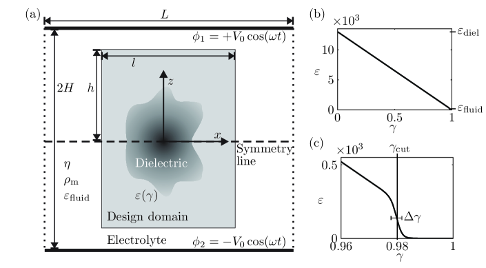
Figure 1: (a) A sketch of the rectangular $L\times 2H$ cross-section of the electrolytic capacitor in the $xz$-plane. The external voltage $\phi_{1}$ and $\phi_{2}$ is applied to the two infinite parallel-plate electrodes (thick black lines) at $z=\pm H$. The voltage difference $\phi_{1}-\phi_{2}$ induces an ICEO flow around the un-biased dielectric solid (dark gray) shaped by the topology optimization routine limited to the rectangular $l\times 2h$ design domain (light gray). The dielectric solid is surrounded by pure electrolyte (light gray and white). Periodic boundary conditions are applied ar the vertical edges (dotted lines). (b) The dimensionless electric permittivity $\varepsilon$ as a function of the design variable $\gamma$. (c) Zoom-in on the rapid convergence of $\varepsilon(\gamma)$ towards $\varepsilon_{\mathrm{fluid}}=1$ for $\gamma$ approaching unity after passing the value $\gamma_{\mathrm{cut}}-\Delta\gamma\simeq 0.98$.

3 Governing equations

We follow the conventional continuum approach to the electrokinetic modeling of the electrolytic capacitor [3]. For simplicity we consider a symmetric, binary electrolyte, where the positive and negative ions with concentrations $c_{+}$ and $c_{-}$, respectively, have the same diffusivity $D$ and valence charge number $Z$.

3.1 Bulk equations in the conventional ICEO model

Neglecting chemical reactions in the bulk of the electrolyte, the ionic transport is governed by particle conservation through the continuity equation,

$$\frac{\partial c_{\pm}}{\partial t}=-\bm{\nabla}\cdot\bm{J}_{\pm},$$ (1)

where $\bm{J}_{\pm}$ is the flux density of the two ionic species, respectively. Assuming a dilute electrolytic solution, the ion flux densities are governed by the Nernst–Planck equation,

$$\bm{J}_{\pm}=-D\bigg{(}\bm{\nabla}c_{\pm}+\frac{\pm Ze}{k_{\mathrm{B}}T}c_{\pm}\bm{\nabla}\phi\bigg{)},$$ (2)

where the first term expresses ionic diffusion and the second term ionic electro-migration due to the electrostatic potential $\phi$. Here $e$ is the elementary charge, $T$ the absolute temperature and $k_{\mathrm{B}}$ the Boltzmann constant. We note that due to the low fluid velocity $\bm{v}$ obtained in the ICEO systems under consideration, we can safely neglect the convective ion fluxes $c_{\pm}\bm{v}$ throughout this paper, see Table 2.

The electrostatic potential $\phi$ is determined by the charge density $\rho_{\mathrm{el}}=Ze(c_{+}-c_{-})$ through Poisson’s equation,

$$\bm{\nabla}\cdot(\varepsilon_{\mathrm{fluid}}\bm{\nabla}\phi)=-\rho_{\mathrm{el}},$$ (3)

where $\varepsilon_{\mathrm{fluid}}$ is the fluid permittivity, which is assumed constant. The fluid velocity field $\bm{v}$ and pressure field $p$ are governed the the continuity equation and the Navier–Stokes equation for incompressible fluids,

$$\bm{\nabla}\cdot\bm{v}=0,$$ (4a)

$$\rho_{\mathrm{m}}\bigg{[}\frac{\partial\bm{v}}{\partial t}+(\bm{v}\cdot\bm{\nabla})\bm{v}\bigg{]}=-\bm{\nabla}p+\eta\nabla^{2}\bm{v}-\rho_{\mathrm{el}}\bm{\nabla}\phi,$$ (4b)

where $\rho_{\mathrm{m}}$ and $\eta$ are the fluid mass density and viscosity, respectively, both assumed constant.

3.2 The artificial design field $\gamma$ used in the topology optimization model of ICEO

To be able to apply the method of topology optimization, it is necessary to extend the conventional ICEO model with three additional terms, all functions of a position-dependent artificial design field $\gamma(\bm{r})$. The design field varies continuously from zero to unity, where $\gamma=0$ is the limit of a pure dielectric solid and $\gamma=1$ is the limit of a pure electrolytic fluid. The intermediate values of $\gamma$ represent a mixture of solid and fluid.

The first additional term concerns the purely fluid dynamic part of our problem. Here, we follow Borrvall and Petersson [6] and model the dielectric solid as a porous medium giving rise to a Darcy friction force density $-\alpha(\gamma)\bm{v}$, where $\alpha(\gamma)$ may be regarded as a local inverse permeability, which we denote the Darcy friction. We let $\alpha(\gamma)$ be a linear function of $\gamma$ of the form $\alpha(\gamma)=\alpha_{\mathrm{max}}(1-\gamma)$, where $\alpha_{\mathrm{max}}=\eta/\ell_{\mathrm{pore}}^{2}$ is the Darcy friction of the porous dielectric material assuming a characteristic pore size $\ell_{\mathrm{pore}}$. In the limit of a completely impenetrable solid the value of $\alpha_{\mathrm{max}}$ approaches infinity, which leads to a vanishing fluid velocity $\bm{v}$. The modified Navier–Stokes equation extending to the entire domain, including the dielectric material, becomes

$$\rho_{\mathrm{m}}\bigg{[}\frac{\partial\bm{v}}{\partial t}+(\bm{v}\cdot\bm{\nabla})\bm{v}\bigg{]}=-\bm{\nabla}p+\eta\nabla^{2}\bm{v}-\rho_{\mathrm{el}}\bm{\nabla}\phi-\alpha(\gamma)\bm{v}.$$ (4e)

The second additional term is specific to our problem. Since the Navier–Stokes equation is now extended to include also the porous dielectric medium, our model must prevent the unphysical penetration of the electrolytic ions into the solid. Following the approach of Kilic et al. [13], where current densities are expressed as gradients of chemical potentials, $\bm{J}\propto-\bm{\nabla}\mu$, we model the ion expulsion by adding an extra free energy term $\kappa(\gamma)$ to the chemical potential $\mu_{\pm}=\pm Ze\phi+k_{\mathrm{B}}T\ln(c_{\pm}/c_{0})+\kappa(\gamma)$ of the ions, where $c_{0}$ is the bulk ionic concentration for both ionic species. As above we let $\kappa(\gamma)$ be a linear function of $\gamma$ of the form $\kappa(\gamma)=\kappa_{\mathrm{max}}(1-\gamma)$, where $\kappa_{\mathrm{max}}$ is the extra energy cost for an ion to enter a point containing a pure dielectric solid as compared to a pure electrolytic fluid. The value of $\kappa_{\mathrm{max}}$ is set to an appropriately high value to expel the ions efficiently from the porous material while still ensuring a smooth transition from dielectric solid to electrolytic fluid. The modified ion flux density becomes

$$\bm{J}_{\pm}=-D\bigg{(}\bm{\nabla}c_{\pm}+\frac{\pm Ze}{k_{\mathrm{B}}T}c_{\pm}\bm{\nabla}\phi+\frac{1}{k_{\mathrm{B}}T}c_{\pm}\bm{\nabla}\kappa(\gamma)\bigg{)}.$$ (4f)

The third and final additional term is also specific to our problem. Electrostatically, the transition from the dielectric solid to the electrolytic fluid is described through the Poisson equation by a $\gamma$-dependent permittivity $\varepsilon(\gamma)$. This modified permittivity varies continuously between the value $\varepsilon_{\mathrm{diel}}$ of the dielectric solid and $\varepsilon_{\mathrm{fluid}}$ of the electrolytic fluid. As above, we would like to choose $\varepsilon(\gamma)$ to be a linear function of $\gamma$. However, during our analysis using a metallic dielectric with $\varepsilon_{\mathrm{diel}}=10^{6}\varepsilon_{0}$ in an aqueous electrolyte with $\varepsilon_{\mathrm{fluid}}=78\>\varepsilon_{0}$ we found unphysical polarization phenomena in the electrolyte due to numerical rounding-off errors for $\gamma$ near, but not equal to, unity. To overcome this problem we ensured a more rapid convergence towards the value $\varepsilon_{\mathrm{fluid}}$ by introducing a cut-off value $\gamma_{\mathrm{cut}}\simeq 0.98$, a transition width $\Delta\gamma\simeq 0.002$, and the following expression for $\varepsilon(\gamma)$,

$$\varepsilon(\gamma)=\varepsilon_{\mathrm{diel}}+(\varepsilon_{\mathrm{fluid}}-\varepsilon_{\mathrm{diel}})\bigg{\{}1-\frac{(1\!-\!\gamma)}{2}\Big{[}\tanh\!\Big{(}\frac{\gamma_{\mathrm{cut}}\!-\!\gamma}{\Delta\gamma}\Big{)}+1\Big{]}\bigg{\}}.$$ (4g)

For $\gamma\lesssim\gamma_{\mathrm{cut}}$ we obtain the linear relation $\varepsilon(\gamma)=\varepsilon_{\mathrm{diel}}+(\varepsilon_{\mathrm{fluid}}-\varepsilon_{\mathrm{diel}})\gamma$, while for $\gamma\gtrsim\gamma_{\mathrm{cut}}$ we have $\varepsilon(\gamma)=\varepsilon_{\mathrm{fluid}}$, see Fig. 1(b)-(c). For $\gamma$ sufficiently close to unity (and not only when $\gamma$ equals unity with numerical precision), this cut-off procedure ensures that the calculated topological break up of the dielectric solid indeed leads to several correctly polarized solids separated by pure electrolyte. The modified Poisson equation becomes

$$\bm{\nabla}\cdot\big{[}\varepsilon(\gamma)\bm{\nabla}\phi\big{]}=-\rho_{\mathrm{el}}.$$ (4h)

Finally, we introduce the $\gamma$-dependent quantity, the so-called objective function $\Phi[\gamma]$, to be optimized by the topology optimization routine: the flow rate in the $x$-direction perpendicular to the applied potential gradient. Due to incompressibility, the flow rate $Q(x)$ is the same through cross-sections parallel to the $yz$-plane at any position $x$. Hence we can use the numerically more stable integrated flow rate as the objective function,

$$\Phi[\gamma(\bm{r})]=\int_{0}^{L}Q(x)\>\mathrm{d}x=\int_{\Omega}\bm{v}\cdot\hat{\bm{n}}_{x}\>\mathrm{d}x\>\mathrm{d}z,$$ (4i)

where $\Omega$ is the entire geometric domain (including the design domain), and $\hat{\bm{n}}_{x}$ the unit vector in the $x$ direction.

3.3 Dimensionless form

To prepare the numerical implementation, the governing equations are rewritten in dimensionless form, using the characteristic parameters of the system. In conventional ICEO systems the size $a$ of the dielectric solid is the natural choice for the characteristic length scale $\ell_{0}$, since the generated slip velocity at the solid surface is proportional to $a$. However, when employing topology optimization we have no prior knowledge of this length scale, and thus we choose it to be the fixed geometric half-length $\ell_{0}=H$ between the capacitor plates. Further characteristic parameters are the ionic concentration $c_{0}$ of the bulk electrolyte, and the thermal voltage $\phi_{0}=k_{\mathrm{B}}T/(Ze)$. The characteristic velocity $u_{0}$ is chosen as the Helmholtz–Smoluchowski slip velocity induced by the local electric field $E=\phi_{0}/\ell_{0}$, and finally the pressure scale is set by the characteristic microfluidic pressure scale $p_{0}=\eta u_{0}/\ell_{0}$.

Although strictly applicable only to parallel-plate capacitors, the characteristic time $\tau_{0}$ of the general system in chosen as the RC time of the double layer in terms of the Debye length $\lambda_{\mathrm{D}}$ of the electrolyte [14],

$$\tau_{0}=\frac{\ell_{0}}{D}\>\lambda_{\mathrm{D}}=\frac{\ell_{0}}{D}\>\sqrt{\frac{k_{\mathrm{B}}T\varepsilon_{\mathrm{fluid}}}{2(Ze)^{2}c_{0}}}.$$ (4j)

Moreover, three characteristic numbers are connected to the $\gamma$-dependent terms in the governing equations: The characteristic free energy $\kappa_{0}$, the characteristic permittivity chosen as the bulk permittivity $\varepsilon_{\mathrm{fluid}}$, and the characteristic Darcy friction coefficient $\alpha_{0}$. In summary,

$$\ell_{0}=H,\qquad\phi_{0}=\frac{k_{\mathrm{B}}T}{Ze},\quad u_{0}=\frac{\varepsilon_{\mathrm{fluid}}\phi_{0}^{2}}{\eta\,\ell_{0}},\quad p_{0}=\frac{\eta\,u_{0}}{\ell_{0}},$$ (4ka)

$$\tau_{0}=\frac{\ell_{0}\lambda_{\mathrm{D}}}{D},\quad\;\omega=\frac{2\pi}{\tau_{0}},\quad\;\;\;\kappa_{0}=k_{\mathrm{B}}T,\qquad\alpha_{0}=\frac{\eta}{\ell_{0}^{2}}.$$ (4kb)

The new dimensionless variables (denoted by a tilde) thus become

$$\tilde{\bm{r}}=\frac{\bm{r}}{\ell_{0}},\quad\tilde{\bm{v}}=\frac{\bm{v}}{u_{0}},\quad\tilde{p}=\frac{p}{p_{0}},\quad\;\tilde{\phi}=\frac{\phi}{\phi_{0}},\quad\tilde{c}_{\pm}=\frac{c_{\pm}}{c_{0}},$$ (4kla)

$$\tilde{t}=\frac{t}{\tau_{0}},\quad\;\tilde{\kappa}=\frac{\kappa}{\kappa_{0}},\quad\tilde{\alpha}=\frac{\alpha}{\alpha_{0}},\quad\tilde{\varepsilon}=\frac{\varepsilon}{\varepsilon_{\mathrm{fluid}}}.$$ (4klb)

In the following all variables and parameters are made dimensionless using these characteristic numbers and for convenience the tilde is henceforth omitted.

3.4 Linearized and reformulated equations

To reduce the otherwise very time and memory consuming numerical simulations, we choose to linearize the equations. There are several nonlinearities to consider.

By virtue of a low Reynolds number $\textit{Re}\approx 10^{-6}$, see Table 2, the nonlinear Navier–Stokes equation is replaced by the linear Stokes equation. Likewise, as mentioned in Sec. 3.1, the low Péclet number $\textit{P\'{e}}\approx 10^{-3}$ allows us to neglect the nonlinear ionic convection flux density $c_{\pm}\bm{v}$. This approximation implies the additional simplification that the electrodynamic problem is independent of the hydrodynamics.

Finally, since $Ze\zeta/k_{\mathrm{B}}T\lesssim 0.5$ the linear Debye–Hückel approximation is valid, and we can utilize that the ionic concentrations only deviate slightly from the bulk equilibrium ionic concentration. The governing equations are reformulated in terms of the average ion concentration $c\equiv(c_{+}+c_{-})/2$ and half the charge density $\rho\equiv(c_{+}-c_{-})/2$. Thus, by expanding the fields to first order as $c=1+\delta c$ and $\rho=0+\delta\rho$, the resulting differential equation for $\rho$ is decoupled from that of $c$. Introducing complex field notation, the applied external bias voltage is $\Delta\phi(t)=2V_{0}\cos(\omega t)=\mathrm{Re}[2V_{0}\exp(\mathrm{i}\omega t)]$, yielding a corresponding response for the potential $\phi$ and charge density $\rho$, with the complex amplitudes $\Phi(\bm{r})=\Phi_{R}(\bm{r})+\mathrm{i}\Phi_{I}(\bm{r})$ and $P(\bm{r})=P_{R}(\bm{r})+\mathrm{i}P_{I}(\bm{r})$, respectively. The resulting governing equations for the electrodynamic problem is then

$$\qquad\qquad\quad\bm{\nabla}\cdot\big{[}\varepsilon(\gamma)\bm{\nabla}\Phi_{R}\big{]} =-\frac{1}{\epsilon^{2}}P_{R},$$ (4klma)

$$\qquad\qquad\quad\bm{\nabla}\cdot\big{[}\varepsilon(\gamma)\bm{\nabla}\Phi_{I}\big{]} =-\frac{1}{\epsilon^{2}}P_{I},$$ (4klmb)

$$\bm{\nabla}\cdot\big{[}\bm{\nabla}\Phi_{R}+\bm{\nabla}P_{R}+P_{R}\bm{\nabla}\kappa(\gamma)\big{]} =-\frac{\omega}{\epsilon}P_{I},$$ (4klmc)

$$\bm{\nabla}\cdot\big{[}\bm{\nabla}\Phi_{I}+\bm{\nabla}P_{I}+P_{I}\bm{\nabla}\kappa(\gamma)\big{]} =+\frac{\omega}{\epsilon}P_{R},$$ (4klmd)

where we have introduced the dimensionless thickness of the linear Debye layer $\epsilon=\lambda_{\mathrm{D}}/\ell_{0}$. Given the electric potential $\Phi$ and the charge density $P$, we solve for the time-averaged hydrodynamic fields $\langle\bm{v}\rangle$ and $\langle p\rangle$,

$$\bm{\nabla}\cdot\langle\bm{v}\rangle =0,$$ (4klmna)

$$\qquad 0 =-\bm{\nabla}\langle p\rangle+\nabla^{2}\langle\bm{v}\rangle+\langle\bm{f}_{\mathrm{el}}\rangle-\alpha(\gamma)\langle\bm{v}\rangle,$$ (4klmnb)

where the time-averaged electric body force density $$\langle\bm{f}_{\mathrm{el}}\rangle$$ is given by

$$\quad\langle\bm{f}_{\mathrm{el}}\rangle=-\frac{1}{2\epsilon^{2}}\big{[}P_{R}\bm{\nabla}\Phi_{R}+P_{I}\bm{\nabla}\Phi_{I}\big{]}.$$ (4klmnc)

3.5 Boundary conditions

For symmetric dielectric solids we exploit the symmetry around $z=0$ and consider only the upper half $(0<z<1)$ of the domain. As boundary condition on the driving electrode we set the amplitude $V_{0}$ of the applied potential. Neglecting any electrode reactions taking place at the surface there is no net ion flux in the normal direction to the boundary with unit vector $\hat{\bm{n}}$. For the fluid velocity we set a no-slip condition, and thus at $z=1$ we have

$$\Phi_{R}=V_{0},\quad\Phi_{I}=0,$$ (4klmnoa)

$$\hat{\bm{n}}\cdot\big{[}\bm{\nabla}\Phi_{R}+\bm{\nabla}P_{R}+P_{R}\bm{\nabla}\kappa(\gamma)\big{]}=0,$$ (4klmnob)

$$\hat{\bm{n}}\cdot\big{[}\bm{\nabla}\Phi_{I}+\bm{\nabla}P_{I}+P_{I}\bm{\nabla}\kappa(\gamma)\big{]}=0,$$ (4klmnoc)

$$\langle\bm{v}\rangle=\bm{0}.$$ (4klmnod)

On the symmetry axis ($z=0$) the potential and the charge density must be zero due to the anti-symmetry of the applied potential. Furthermore, there is no fluid flux in the normal direction and the shear stresses vanish. So at $x=0$ we have

$$\Phi_{R}=\Phi_{I}=0,\quad P_{R}=P_{I}=0,$$ (4klmnopa)

$$\hat{\bm{n}}\cdot\langle\bm{v}\rangle=0,\quad\hat{\bm{t}}\cdot\langle\bm{\sigma}\rangle\cdot\hat{\bm{n}}=0,$$ (4klmnopb)

where the dimensionless stress tensor is $\langle\sigma_{ik}\rangle=-\langle p\rangle\delta_{ik}+\big{(}\partial_{i}\langle v_{k}\rangle+\partial_{k}\langle v_{i}\rangle\big{)}$, and $\hat{\bm{n}}$ and $\hat{\bm{t}}$ are the normal and tangential unit vectors, respectively, where the latter in 2D, contrary to 3D, is uniquely defined. On the remaining vertical boundaries ($x=\pm L/2\ell_{0}$) periodic boundary conditions are applied to all the fields.

Corresponding boundary conditions apply to the conventional ICEO model Eqs. (1)-(4b), without the artificial design field but with a hard-wall dielectric solid. For the boundary between a dielectric solid and and electrolytic fluid the standard electrostatic conditions apply, moreover, there is no ion flux normal to the surface, and a no-slip condition is applied to the fluid velocity.

Table 1: Parameters used in the simulations of the topology optimization ICEO model and the conventional ICEO model.

Parameter	Symbol	Dimensionless	Physical
		value	value
Characteristic length	$\ell_{0}$	$1.0$	$250~{}\mathrm{nm}$
Channel half-height	$H$	$1.0$	$250~{}\mathrm{nm}$
Channel length	$L$	$2.0$	$500~{}\mathrm{nm}$
Design domain half-height	$h$	$0.8$	$200~{}\mathrm{nm}$
Design domain length	$l$	$0.6$	$150~{}\mathrm{nm}$
Linear Debye length	$\lambda_{\mathrm{D}}$	$0.08$	$20~{}\mathrm{nm}$
Characteristic velocity	$u_{0}$	$1.0$	$1.7\times 10^{-3}~{}\mathrm{m/s}$
Characteristic potential	$\phi_{0}$	$1.0$	$25~{}\mathrm{mV}$
External potential amplitude	$V_{0}$	$1.0$	$25~{}\mathrm{mV}$
External potential frequency	$\omega$	$6.28$	$4\times 10^{5}~{}\mathrm{rad/s}$
Bulk fluid permittivity	$\varepsilon_{\mathrm{fluid}}$	$1.0$	$78\>\varepsilon_{0}$
Dielectric permittivity	$\varepsilon_{\mathrm{diel}}$	$1.3\times 10^{4}$	$10^{6}\>\varepsilon_{0}$
Bulk ionic concentration	$c_{0}$	$1.0$	$0.23~{}\mathrm{mM}$
Fluid viscosity	$\eta$	$1.0$	$10^{-3}~{}\mathrm{Pa\,s}$
Ionic diffusion constant	$D$	$1.0$	$2\times 10^{-9}\mathrm{m}^{2}/\mathrm{s}$
Ionic free energy in solid	$\kappa$	$3.0$	$75~{}\mathrm{mV}$
Maximum Darcy friction	$\alpha_{\mathrm{max}}$	$10^{5}$	$2\times 10^{16}~{}\mathrm{Pa\>s/m}^{2}$

4 Implementation and validation of numerical code

4.1 Implementation and parameter values

For our numerical analysis we use the commercial numerical finite-element modeling tool Comsol [16] controlled by scripts written in Matlab [15]. The mathematical method of topology optimization in microfluidic systems is based on the seminal paper by Borrvall and Petersson [6], while the implementation containing the method of moving asymptotes by Svanberg [17, 18] is taken from Olesen, Okkels and Bruus [7].

Due to the challenges discussed in Sec. 4.2 of resolving all length scales in the electrokinetic model, we have chosen to study small systems, $2H=500$ nm, with a relatively large Debye length, $\lambda_{\mathrm{D}}=20$ nm. Our main goal is to provide a proof of concept for the use of topology optimization in electro-hydrodynamic systems, so the difficulties in fabricating actual devices on this sub-micrometric scale is not a major concern for us in the present work. A list of the parameter values chosen for our simulations is given in Table 1.

For a typical topology optimization, as the one shown in Fig. 3(a), approximately 5400 FEM elements are involved. In each iteration loop of the topology optimization routine three problems are solved: the electric problem , the hydrodynamic problem, and the adjunct problem for the sensitivity analysis, involving $4\times 10^{4}$ , $2\times 10^{4}$ , and $7\times 10^{4}$ degrees of freedom, respectively. On an Intel Core 2 Duo 2 GHz processer with 2 GB RAM the typical CPU time is several hours.

4.2 Analytical and numerical validation by the conventional ICEO model

We have validated our simulations in two steps. First, the conventional ICEO model not involving the design field $\gamma(\bm{r})$ is validated against the analytical result for the slip velocity at a simple dielectric cylinder in an infinite AC electric field given by Squires and Bazant [3]. Second, the design field model is compared to the conventional model. This two-step validation procedure is necessary because of the limited computer capacity. The involved length scales in the problem make a large number of mesh elements necessary for the numerical solution by the finite element method. Four different length scales appear in the gamma-dependent model for the problem of a cylinder placed mid between the parallel capacitor plates: The distance $H$ from the center of the dielectric cylinder to the biased plates, the radius $a$ of the cylinder, the Debye length $\lambda_{\mathrm{D}}$, and the length $d$ over which the design field $\gamma$ changes from zero to unity. This last and smallest length-scale $d$ in the problem is controlled directly be the numerical mesh size set up in the finite element method. It has to be significantly smaller than $\lambda_{\mathrm{D}}$ to model the double layer dynamics correctly, so here a maximum value of the numerical mesh size is defined.

The analytical solution of Squires and Bazant [3] is only strictly valid in the case of an infinitely thin Debye layer in an infinite electric field. So, to compare this model with the bounded numerical model the plate distance must be increased to minimize the influence on the effective slip velocity. Furthermore, it has been shown in a numerical study of Gregersen et al. [19] that the Debye length $\lambda_{\mathrm{D}}$ should be about a factor of $10^{3}$ smaller than the cylinder radius $a$ to approximate the solution for the infinitely thin Debye layer model. Including the demand of $d$ being significantly smaller than $\lambda_{\mathrm{D}}$ we end up with a length scale difference of at least $10^{5}$, which is difficult to resolve by the finite element mesh, even when mesh adaption is used. Consequently, we have checked that the slip velocity for the conventional model converges towards the analytical value when the ratio $\lambda_{\mathrm{D}}/a$ decreases. Afterwards, we have compared the solutions for the conventional and gamma-dependent models in a smaller system with a ratio of $\lambda_{\mathrm{D}}/a\sim 10$ and found good agreement.

4.3 Validation of the self-consistency of the topology optimization

As an example of our validation of the self-consistency of the topology optimization, we study the dependence of the objective function $Q=\Phi[\omega,\gamma(\omega,\bm{r})]$ on the external driving frequency $\omega$. As shown in Fig. 2(a)-(c) we have calculated the topology optimized dielectric structures $\gamma_{j}=\gamma(\omega_{j},\bm{r})$, $j=a,b,c$, for three increasing frequencies $\omega=\omega_{a}=1.25$, $\omega=\omega_{b}=12.5$, and $\omega=\omega_{c}=62.5$. In the following we let $Q_{j}(\omega)$ denote the flow rate calculated at the frequency $\omega$ for a structure optimized at the frequency $\omega_{j}$.

First, we note that $Q_{j}(\omega_{j})$ decreases as the frequency increases above the characteristic frequency $\omega_{0}=1$; $Q_{a}(\omega_{a})=2.95\times 10^{-3}$, $Q_{b}(\omega_{b})=1.82\times 10^{-3}$, and $Q_{c}(\omega_{c})=0.55\times 10^{-3}$. This phenomenon is a general aspect of ICEO systems, where the largest effect is expected to happen at $\omega=2\pi/\tau_{0}=6.28$.

Second, and most significant, we see in Fig. 2(d) that structure $\gamma_{a}$ is indeed the optimal structure for $\omega=\omega_{a}$ since $Q_{a}(\omega_{a})>Q_{b}(\omega_{a}),Q_{c}(\omega_{a})$. Likewise, $\gamma_{b}$ is optimal for $\omega=\omega_{b}$, and $\gamma_{c}$ is optimal for $\omega=\omega_{c}$.

We have gained confidence in the self-consistency of our topology optimization routine by carrying out a number of tests like the one in the example above.

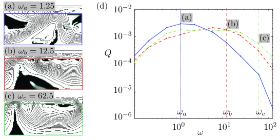
Figure 2: Validation of the self-consistency of the topology optimization for different driving frequencies $\omega$. (a) The streamline pattern (thick lines) for $\omega=\omega_{a}=1.25$ calculated using the design-field ICEO model with a porous dielectric medium (black and gray), the structure $\gamma_{a}$ of which has been found by topology optimization within the indicated rectangular design domain (straight lines). The flow rate for this converged solution structure is $Q=2.95\times 10^{-3}$. (b) As panel (a) but with $\omega=\omega_{b}=12.5$ and $Q=1.82\times 10^{-3}$. (c) As panel (a) but with $\omega=\omega_{c}=62.5$ and $Q=0.55\times 10^{-3}$. (d) Flow rate $Q$ versus frequency $\omega$ for each of the three structures in panel (a), (b), and (c). Note that structure $\gamma_{a}$ indeed yields the highest flow rate $Q$ for $\omega=\omega_{a}$, structure $\gamma_{b}$ maximizes $Q$ for $\omega=\omega_{b}$, and structure $\gamma_{c}$ maximizes $Q$ for $\omega=\omega_{c}$.

5 Results

Figure 3: (a) The streamline pattern (thick lines) calculated for $\omega=6.28$ using the design-field ICEO model with a porous dielectric medium (black and gray), the structure of which has been find by topology optimization within the indicated rectangular design domain (thin lines). The flow rate for this converged solution structure is $Q=2.99\times 10^{-3}$. (b) The streamline pattern (full lines) calculated using the conventional ICEO model with a hard-walled dielectric solid (black). The shape of the dielectric solid is the 0.95-contour of the $\gamma$-field taken from the topology-optimized structure shown in panel (a). The flow rate is $Q=Q^{*}=1.88\times 10^{-3}$. (c) and (d) Color plot of the charge density $\rho(\bm{r})$ corresponding to panel (a) and (b), respectively. See Table 1 for parameter values.

5.1 Topology optimization

For each choice of parameters the topology optimization routine converges to a specific distribution of dielectric solid given by $\gamma(\bm{r})$. As a starting point for the investigation of the optimization results we used the parameters listed in Table 1. As discussed above, the geometric dimensions are chosen as large as possible within the computational limitations: the Debye length is set to $\lambda_{\mathrm{D}}=20~{}\mathrm{nm}$ and the distance between the capacitor plates to $2H=500~{}\mathrm{nm}$. The external bias voltage is of the order of the thermal voltage $V_{0}=25$ mV to ensure the validity of the linear Debye–Hückel approximation. We let the bulk fluid consist of water containing small ions, such as dissolved KCl, with a concentration $c_{0}=0.23$ mM set by the chosen Debye length. The dielectric material permittivity is set to $\varepsilon_{\mathrm{diel}}=10^{6}\>\varepsilon_{0}$ in order to mimic the characteristics of a metal. The artificial parameters $\kappa$ and $\alpha_{\mathrm{max}}$ are chosen on a pure computational basis, where they have to mimic the real physics in the limits of fluid and solid, but also support the optimization routine when the phases are mixed.

Table 2: The value of characteristic physical quantities calculated in the topology optimization ICEO model corresponding to Fig. 3.

Quantity	Symbol	Dimensionless	Physical
		value	value
Gap between dielectric pieces	$\ell_{\mathrm{gap}}$	$0.4$	$100~{}\mathrm{nm}$
Velocity in the gap	$u_{\mathrm{gap}}$	$0.016\>u_{0}$	$28~{}\mu\mathrm{m/s}$
Largest zeta potential	$\zeta_{\mathrm{max}}$	$0.5\>\phi_{0}$	$12.5~{}\mathrm{mV}$
Reynolds number Re	$\rho_{\mathrm{m}}u_{\mathrm{gap}}\ell_{\mathrm{gap}}/\eta$	$2.8\times 10^{-6}$	$-$
Péclet number Pé	$u_{\mathrm{gap}}\ell_{\mathrm{gap}}/D$	$1.4\times 10^{-3}$	$-$
Debye–Hückel number Hü	$e\zeta_{\mathrm{max}}/(4k_{\mathrm{B}}T)$	$0.13$	$-$

Throughout our simulations we have primarily varied the applied frequency $\omega$ and the size $l\times 2h$ of the design domain. In Fig. 2 we have shown examples of large design domains with $l\times h=2.0\times 0.8$ covering 80% of the entire domain and frequency sweeps over three orders of magnitude. However, in the following we fix the frequency to be $\omega=2\pi/\tau_{0}=6.28$, where the ICEO response is maximum. Moreover we focus on a smaller design domain $l\times h=0.6\times 0.8$ to obtain better spatial resolution for the given amount of computer memory and to avoid getting stuck in local optima. It should be stressed that the size of the design domain has a large effect on the specific form and size of the dielectric islands produced by the topology optimization. Also, it is important if the design domain is allowed to connect to the capacitor plates or not, see the remarks in Sec. 6.

The converged solution found by topology optimization under these conditions is shown in Fig. 3(a). The shape of the porous dielectric material is shown together with a streamline plot of equidistant contours of the flow rate. We notice that many stream lines extend all the way through the domain from left to right indicating that a horizontal flow parallel to the $x$-axis is indeed established. The resulting flow rate is $Q=2.99\times 10^{-3}$. The ICEO flow of this solution, based on the design-field model, is validated by transferring the geometrical shape of the porous dielectric medium into a conventional ICEO model with a hard-walled dielectric not depending on the design field. In the latter model the sharp interface between the dielectric solid and the electrolyte is defined by the 0.95-contour of the topology optimized design field $\gamma(\bm{r})$. The resulting geometry and streamline pattern of the conventional ICEO model is shown in Fig. 3(b). The flow rate is now found to be $Q=Q^{*}=1.88\times 10^{-3}$. There is a close resemblance between the results of two models both qualitatively and quantitatively. It is noticed how the number and positions of the induced flow rolls match well, and also the absolute values of the induced horizontal flow rates differs only by 37%.

Based on the simulation we can now justify the linearization of our model. The largest velocity $u_{\mathrm{gap}}$ is found in the gap of width $\ell_{\mathrm{gap}}$ between the two satellite pieces and the central piece. As listed in Table 2 the resulting Reynolds number is $\textit{Re}=2.8\times 10^{-7}$, the Péclet number is $\textit{P\'{e}}=1.4\times 10^{-3}$, while the Debye–Hückel number is $\textit{H\"{u}}=0.13$.

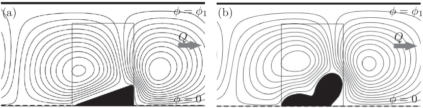
Figure 4: (a) The streamline pattern (thick lines) for a simple triangular reference structure calculated for $\omega=6.28$ using the conventional ICEO model with a hard-walled dielectric solid (black). The height $b=0.32$ of the triangle is chosen to give the largest flow rate for a fixed base line given by the rectangular design domain of Fig. 3(a). The flow rate is $Q=0.22\times 10^{-3}$. (b) The same as panel (a) except the geometry of the dielectric solid is given by the perturbed circle $r(\theta)=0.24[1+0.5\cos(3\theta)]$. The flow rate is $Q=0.46\times 10^{-3}$.

5.2 Comparison to simple shapes

We evaluate our result for the optimized flow rate by comparing it to those obtained for more basic, simply connected, dielectric shapes, such as triangles and perturbed circles previously studied in the literature as flow inducing objects both analytically and experimentally [3, 4, 5]. For comparison, such simpler shapes have been fitted into the same design domain as used in the topology optimization Fig. 3(a), and the conventional ICEO model without the design field was solved for the same parameter set. In Fig. 4(a) the resulting flow for a triangle with straight faces and rounded corners is shown. The height $b$ of the face perpendicular to the symmetry line was varied within the height of the design domain $0<b<0.8$, and the height $b=0.32$ generating the largest flow in the $x$-direction results in a flow rate of $Q=0.22\times 10^{-3}$, which is eight times smaller than the topology optimized result. In Fig. 4(b) the induced flow around a perturbed cylinder with radius $r(\theta)=0.24\big{[}1+0.5\cos(3\theta)\big{]}$ is depicted. Again the shape has been fitted within the allowed design domain. The resulting flow rate $Q=0.46\times 10^{-3}$ is higher than for the triangle but still a factor of four slower than the optimized result. It is clearly advantageous to change the topology of the dielectric solid from simply to multiply connected.

For the topology optimized shape in Fig. 3(a) it is noticed that only a small amount of flow is passing between the two closely placed dielectric islands in the upper left corner of the design domain. To investigate the importance of this separation, the gap between the islands was filled out with dielectric material and the flow calculated. It turns out that this topological change only lowered the flow rate slightly ($15\%$) to a value of $Q=1.59\times 10^{-3}$. Thus, the important topology of the dielectric solid in the top-half domain is the appearance of one center island crossing the antisymmetry line and one satellite island near the tip of the center island.

5.3 Shape optimization

The topology optimized solutions are found based on the extended ICEO model involving the artificial design field $\gamma(\bm{r})$. To avoid the artificial design field it is desirable to validate and further investigate the obtained topology optimized results by the physically more correct conventional ICEO model involving hard-walled solid dielectrics. We therefore extend the reasoning behind the comparison of the two models shown in Fig. 3 and apply a more stringent shape optimization to the various topologies presented above. With this approach we are gaining further understanding of the specific shapes comprising the overall topology of the dielectric solid. Moremore, it is possible to point out simpler shapes, which are easier to fabricate, but still perform well.

In shape optimization the goal is to optimize the objective function $\Phi$, which depends on the position and shape of the boundary between the dielectric solid and the electrolytic fluid. This boundary is given by a line interpolation through a small number of points on the boundary. These control points are in turn given by $N$ design variables $\bm{g}=(g_{1},g_{2},\ldots,g_{N})$, so the objective function of Eq. (4i) depending on the design field $\gamma(\bm{r})$ is now written as $\Phi[\bm{g}]$ depending on the design variables $\bm{g}$,

$$\Phi[\bm{g}]=\int_{\Omega}\bm{v}\cdot\hat{\bm{n}}_{x}\>\mathrm{d}x\>\mathrm{d}z.$$ (4klmnopq)

To carry out the shape optimization we use a direct bounded Nelder-Mead simplex method [20] implemented in Matlab [21, 22]. This robust method finds the optimal point $\bm{g}_{\mathrm{opt}}$ in the $N$-dimensional design variable space by initially creating a simplex in this space, e.g. a $N$-dimensional polyhedron spanned by $N+1$ points, one of which is the initial guess. The simplex then iteratively moves towards the optimal point by updating one of the $N+1$ points at the time. During the iteration, the simplex can expand along favorable directions, shrink towards the best point, or have its worst point replaced with the point obtained by reflecting the worst point through the centroid of the remaining $N$ points. The iteration terminates once the extension of the simplex is below a given tolerance. We note that unlike topology optimization, the simplex method relies only on values of the objective function $\Phi[\bm{g}]$ and not on the sensitivity $\partial\Phi/\partial\bm{g}$ [23].

First, we perform shape optimization on a right-angled triangle corresponding to the one shown in Fig. 4(a). Due to the translation invariance in the $x$-direction, we fix the first basepoint of the triangle $(x_{1},0)$ to the right end of the simulation domain, while the second point $(x_{2},0)$ can move freely along the baseline, in contrast to the original rectangular design. To ensure a right-angled triangle only the $z$-coordinate of the top point $(x_{2},z_{2})$ may move freely. In this case the design variable becomes the two-component vector $\bm{g}=(x_{2},z_{2})$. The optimal right-angled triangle is shown in Fig. 5(a). The flow rate is $Q=0.32\times 10^{-3}$ or 1.5 times larger than that of the original right-angled triangle confined to the design domain.

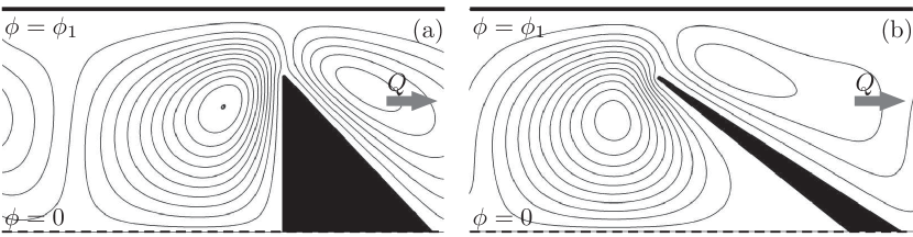
Figure 5: (a) The streamline pattern (thick lines) for the shape-optimized right-angled triangle fixed at the symmetry line $z=0$ calculated for $\omega=6.28$ using the conventional ICEO model with a hard-walled dielectric solid (black). In the full domain this is a triangle symmetric around $z=0$. The flow rate is $Q=0.32\times 10^{-3}$. (b) As in panel (a) but without constraining the triangle to be right-angled. In the full domain the shape is foursided polygon symmetric around $z=0$. The flow rate is $Q=0.76\times 10^{-3}$. Note that all sharp corners of the polygons have been rounded by circular arcs of radius 0.01.

If we do not constrain the triangle to be right-angled, we instead optimize a polygon shape spanned by three corner points in the upper half of the electrolytic capacitor. So, due to the symmetry of the problem, we are in fact searching for the most optimal, symmetric foursided polygon. The three corner points are now given as $(x_{1},0)$, $(x_{2},0)$,and $(x_{3},z_{3})$, and again due to translation invariance, it results in a three-component design variable $\bm{g}=(x_{2},x_{3},z_{3})$. The resulting shape-optimized polygon is shown in Fig. 5(b). The flow rate is $Q=0.76\times 10^{-3}$, which is 3.5 times larger than that of the original right-angled triangle confined to the design domain and 2.4 times better than that of the best right-angled triangle. However, this flow rate is still a factor of 0.4 lower than the topology optimized results.

To be able to shape optimize the more complex shapes of Fig. 3 we have employed two methods to obtain a suitable set of design variables. The first method, the radial method, is illustrated in Fig. 6. The boundary of a given dielectric solid is defined through a cubic interpolation line through $N$ control points $(x_{i},z_{i}),i=1,2,\ldots,N$, which are parameterized in terms of two co-ordinates $(x_{c},z_{c})$ of a center point, two global scale factors $A$ and $B$, $N$ lengths $r_{i}$, and $N$ fixed angles $\theta_{i}$ distributed in the interval from 0 to $2\pi$,

$$(x_{i},z_{i})=(x_{c},z_{c})+r_{i}\>(A\cos\theta_{i},\>B\sin\theta_{i}).$$ (4klmnopr)

In this case the design variable becomes $\bm{g}=(x_{c},z_{c},r_{1},r_{2},\ldots,r_{N},A,B)$.

The second parametrization method involves a decomposition into harmonic components. As before we define a central point $(x_{c},z_{c})$ surrounded by $N$ control points. However now, the distances $r_{i}$ are decomposed into $M$ harmonic components given by

$$r_{i}=r_{0}\bigg{(}1+\sum_{n=1}^{M}A_{n}\cos(n\theta_{i}+\varphi_{n})\bigg{)},$$ (4klmnops)

where $r_{0}$ is an overall scale parameter and $\varphi_{n}$ is a phase shift. In this case the design variable becomes $\bm{g}=(x_{c},z_{c},r_{0},A_{1},A_{2},\ldots,A_{M},\varphi_{1},\varphi_{2},\ldots,\varphi_{M})$.

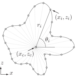
Figure 6: Illustration of the parametrization, Eq. (4klmnopr), of the boundary of a dielectric solid with a complex shape. The polar representation is shown for point $i=7$. The shape consist of five harmonic components represented by Eq. (4klmnops) with the design-variables $x_{c}=-0.1312$, $z_{c}=0.7176$, $r_{0}=0.1403$, $A_{i}=\{0.2501,0.0151,0.0062,0.2103,0.2313\}$, $\varphi_{i}=\{-1.7508,-2.2526,0.4173,0.1172,-0.2419\}$.

5.4 Comparing topology optimization and shape optimization

When shape-optimizing a geometry similar to the one found by topology optimization, we let the geometry consist of two pieces: (i) an elliptic island centered on the symmetry-axis and fixed to the right side of design domain, and (ii) an island with a complex shape to be placed anywhere inside the design domain, but not overlapping with the elliptic island. For the ellipse we only need to specify the major axis $A$ and the minor axis $B$, so these two design parameters add to the design variable listed above for either the radial model or the harmonic decomposition model. To be able to compare with the topology optimized solution the dielectric solid is restricted to the design domain.

The result of this two-piece shape optimization is shown in Fig. 7. Compared to the simply connected topologies, the two-piece shape-optimized systems yields much improved flow rates. For the shape optimization involving the radial method with 16 directional angles and $A=B$ for the complex piece, the flow rate is $Q=1.92\times 10^{-3}$, Fig. 7(a), which is 2.5 times larger than that of the shape-optimized foursided symmetric polygon. The harmonic decomposition method, Fig. 7(b), yields a flow rate of $Q=1.52\times 10^{-3}$ or 2.0 times larger than that of the polygon.

All the results for the obtained flow rates are summarized in Table 3. It is seen that two-piece shape optimized systems performs as good as the topology optimized system, when analyzed using the conventional ICEO model without the artificial design field. We also note by comparing Figs. 3 and 7 that the resulting geometry found using either topology optimization or shape optimization is essentially the same. The central island of the dielectric solid is a thin structure perpendicular to the symmetry axis and covering approximately 60% of the channel width. The satellite island of complex shape is situated near the tip of the central island. It has two peaks pointing towards the central island that seem to suspend a flow roll which guides the ICEO flow through the gap between the two islands.

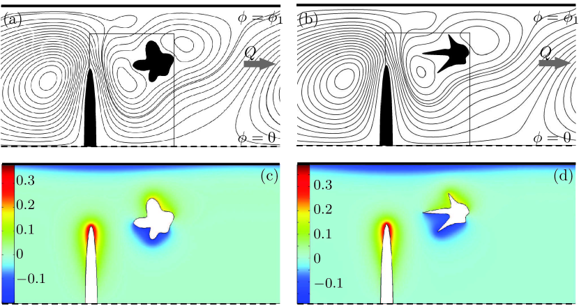
Figure 7: Shape-optimized dielectrics with a topology corresponding to the topology-optimized shapes of Fig. 3. (a) The streamline pattern (thick lines) for a two-piece geometry calculated using the conventional ICEO model. The shape of the hard-walled dielectric solid (black) is found by shape optimization using the radial method Eq. (4klmnopr) with $N=16$ directional angles. The flow rate is $Q=1.92\times 10^{-3}$. (b) The same as panel (a) except the geometry of the dielectric solid is by shape optimization using the harmonic decomposition method Eq. (4klmnops) with $M=5$ modes. The flow rate is $Q=1.52\times 10^{-3}$. (c) and (d) Color plot of the charge density $\rho(\bm{r})$ corresponding to panel (a) and (b), respectively.

Table 3: Overview of the resulting flow rates $Q$ relative to the topology optimized value $Q^{*}=1.88\times 10^{3}$, see Fig. 3(b), for the various geometries analyzed in the conventional ICEO model. The methods by which the geometries have been determined are listed.

Shape	Method	Flow rate
		$Q/Q^{*}$
Triangle with optimal height, Fig. 4(a)	Shape optimization	0.12
Perturbed cylinder, Fig. 4(b)	Fixed shape	0.24
Optimized triangle, Fig. 5(a)	Shape optimization	0.17
Optimized foursided polygon, Fig. 5(b)	Shape optimization	0.40
Topology optimized result, Fig. 3(b)	Topology optimization	1.00
Harmonic decomposition and ellipse, Fig. 7(a)	Shape optimization	0.81
Radial varying points and ellipse, Fig. 7(b)	Shape optimization	1.02

6 Concluding remarks

The main result of this work is the establishment of the topology optimization method for ICEO models extended with the design field $\gamma(\bm{r})$. In contrast to the conventional ICEO model with its sharply defined, impenetrable dielectric solids, the design field ensures a continuous transition between the porous dielectric solid and the electrolytic fluid, which allows for an efficient gradient-based optimization of the problem. By concrete examples we have shown how the use of topology optimization has led to non-trivial system geometries with a flow rate increase of nearly one order of magnitude.

However, there exist many local optima, and we cannot be sure that the converged solution is the global optimum. The resulting shapes and the generated flow rates depend on the initial condition for the artificial $\gamma$-field. Generally, the initial condition used throughout this paper, $\gamma=0.99$ in the entire design domain, leads to the most optimal results compared to other initial conditions. This initial value corresponds to a very weak change from the electrolytic capacitor completely void of dielectric solid. In contrast, if we let $\gamma=0.01$ corresponding to almost pure dielectric material in the entire design region, the resulting shapes are less optimal, i.e. the topology optimization routine is more likely to be caught caught in a local optimum. Furthermore, the resulting shapes turns out to be mesh-dependent as well. So, we cannot conclude much about global optima. Instead, we can use the topology optimized shapes as inspiration to improve existing designs. For this purpose shape optimization turns out to be a powerful tool. We have shown in this work how shape optimization can be used efficiently to refine the shape of the individual pieces of the dielectric solid once its topology has been identified by topology optimization.

For all three additional $\gamma$-dependent fields $\alpha(\gamma)$, $\kappa(\gamma)$, and $\varepsilon(\gamma)$ we have used (nearly) linear functions. In many previous applications of topology optimization non-linear functions have successfully been used to find global optima by gradually changing the non-linearity into strict linearity during the iterative procedure [6, 7, 8, 12]. However, we did not improve our search for a global optimum by employing such schemes, and simply applied the (nearly) linear functions during the entire iteration process.

The limited size of the design domain is in some cases restricting the free formation of the optimized structures. This may be avoided by enlarging the design domain. However, starting a topology optimization in a very large domain gives a huge amount of degrees of freedoms, and the routine is easily caught in local minima. These local minima often yield results not as optimal as those obtained for the smaller design boxes. A solution could be to increase the design domain during the optimization iteration procedure. It should be noted that increasing the box all the way up to the capacitor plates results in solution shapes, where some of the dielectric material is attached to the electrode in order to extend the electrode into the capacitor and thereby maximize the electric field locally. This may be a desirable feature for some purposes. In this work we have deliberately avoided such solutions by keeping the edges of the design domain from the capacitor plates.

Throughout the paper we have only presented results obtained for dielectric solids shapes forced to be symmetric around the center plane $z=0$. However, we have performed both topology optimization and shape optimization of systems not restricted to this symmetry. In general we find that the symmetric shapes always are good candidates for the optimal design. It cannot be excluded, though, that in some cases a spontaneous symmetry breaking occurs similar to the asymmetric S-turn channel studied in Ref. [7].

By studying the optimized shapes of the dielectric solids, we have noted that pointed features often occurs, such as those clearly seen on the dielectric satellite island in Fig. 7(b). The reason for these to appear seems to be that the pointed regions of the dielectric surfaces can support large gradients in the electric potential and associated with this also with large charge densities. As a result large electric body forces act on the electrolyte in these regions. At the same time the surface between the pointed features curve inward which lowers the viscous flow resistance due to the no-slip boundary condition. This effect is similar to that obtained by creating electrode arrays of different heights in AC electro-osmosis [24, 25].

Another noteworthy aspect of the topology optimized structures is that the appearance of dielectric satellite islands seem to break up flow rolls that would otherwise be present and not contribute to the flow rate. This leads to a larger net flow rate, as can be seen be comparing Figs. 4 and 7.

Throughout the paper have treated the design field $\gamma$ as an artificial field. However, the design-field model could perhaps achieve physical applications to systems containing ion exchange membranes, as briefly mentioned in Sec. 1. Such membranes are indeed porous structures permeated by an electrolyte.

In conclusion, our analysis points out the great potential for improving actual ICEO-based devices by changing simply connected topologies and simple shapes of the dielectric solids, into multiply connected topologies of complex shapes.

References

References

- [1] M.Z. Bazant and T. M. Squires, Phys. Rev. Lett. 92 066101 (2004).
- [2] J. A. Levitan, S. Devasenathipathy, V. Studer, Y. Ben, T. Thorsen, T. M. Squires, M. Z. Bazant, a metal wire in a microchannel, Coll. Surf. A 267, 122 (2005).
- [3] T.M. Squires, and M.Z. Bazant, J. Fluid Mech. 509, 217 (2004).
- [4] T.M. Squires, and M.Z. Bazant, J. Fluid Mech. 560, 65 (2006).
- [5] C.K. Harnett, J. Templeton, K. Dunphy-Guzman, Y.M. Senousy, and M.P. Kanouff, Lab Chip 8, 565 (2008).
- [6] T. Borrvall and J. Petersson, Int. J. Numer. Methods Fluids 41, 77 (2003).
- [7] L. H. Olesen, F. Okkels, and H. Bruus, Int. J. Numer. Methods Eng. 65, 975 (2006).
- [8] M.P. Bends e and O. Sigmund, Topology Optimization-Theory, Methods and Applications, Springer (Berlin, 2003).
- [9] J.S. Jensen and O. Sigmund, Appl. Phys. Lett. 84, 2022 (2004).
- [10] M.B. Düring, J.S. Jensen, and O. Sigmund, J. Sound Vib. 317, 557 (2008).
- [11] A. Gersborg-Hansen, O. Sigmund, and R.B. Haber, Struct. Multidiscip. Optim. 30, 181 (2005).
- [12] F. Okkels and H. Bruus, Phys. Rev. E 75, 016301 1–4 (2007).
- [13] M. S. Kilic, M. Z. Bazant, and A. Ajdari, Phys. Rev. E 75, 034702 (2007).
- [14] M. Z. Bazant, K. Thornton, and A. Ajdari, Phys. Rev. E 70, 021506 (2004).
- [15] Matlab, The MathWorks, Inc. (www.mathworks.com).
- [16] Comsol Multiphysics, COMSOL AB (www.comsol.com).
- [17] K. Svanberg, Int. J. Numer. Methods Eng. 24, 359 (1987).
- [18] A MATLAB implementation, mmasub, of the MMAoptimization algorithm [17] can be obtained from Krister Svanberg, KTH, Sweden. E-mail address: krille@math.kth.se.
- [19] M.M. Gregersen, M.B. Andersen, G. Soni, C. Meinhart, T. Squires, H. Bruus, Phys. Rev. E (submitted, 2009).
- [20] J.A. Nelder and R. Mead, Computer Journal, 7, 308 (1965).
- [21] J.C. Lagarias, J.A. Reeds, M.H. Wright, and P.E. Wright, SIAM Journal of Optimization, Vol. 9 No. 1, 112 (1998)
- [22] The routine fminsearch in Matlab version 7 (R14).
- [23] The Matlab function fminsearch is actually unbounded. Therefore the arcus tangent function is used to map the unbounded real axis to the bounded interval of the design variables.
- [24] M.Z. Bazant and Y. Ben, Lab Chip 6, 1455 (2006).
- [25] J. Urbanski, T. Thorsen, J. Levitan, and M. Bazant Appl. Phys. Lett. 89, 143508 (2006).