Experimental evidence for new symmetry axis of electromagnetic beams

Abstract

The new symmetry axis of a well-behaved electromagnetic beam advanced in paper Physical Review A 78, 063831 (2008) is not purely a mathematical concept. The experimental result reported by Hosten and Kwiat in paper Science 319, 787 (2008) is shown to demonstrate the existence of this symmetry axis that is neither perpendicular nor parallel to the propagation axis.

Introduction.—Finite electromagnetic beams have now played very important roles in diverse areas of applications such as optical trapping and manipulation Ashkin , optical rotating Paterson , optical guiding Xu-KJK , optical data storage, and dark-field imaging Biss-YB . But an incredible fact is that the theoretical description of a well-behaved finite beam has not been satisfactory Lax-LM ; Davis ; Pattanayak-A ; Davis-P ; Jordan-H ; Youngworth-B ; Onoda-MN ; Bliokh-B ; Li1 since the advent of masers and lasers Green-W ; Kogelnik ; Kogelnik-L . It is well known that the vectorial property of a plane wave is described by the polarization state. A useful concept is the Jones vector that consists of the two mutually orthogonal transverse components Jones . But for a finite beam, the polarization state is not a global property Pattanayak-A . Instead it is local and changes on propagation. As a matter of fact, due to the longitudinal component Lax-LM ; Li1 , the polarization state is not sufficient to describe the vectorial property of a finite beam. Recently, I advanced a new symmetry axis Li2 represented by a unit vector $\mathbf{I}$ and found that it is a global property and, together with the Jones vector of the angular spectrum, can describe the vectorial property of a beam. The purpose of this paper is to show that this symmetry axis is not purely a mathematical concept. In fact, a perpendicular $\mathbf{I}$ to the propagation axis corresponds to the uniformly polarized beam in the paraxial approximation Davis ; Pattanayak-A , and a parallel $\mathbf{I}$ corresponds to the cylindrical vector beam Davis-P ; Youngworth-B ; Li1 . The conversion from uniformly polarized beams to cylindrical vector beams has been experimentally realized Youngworth-B ; Ren-LW . In this paper, I will show that a symmetry axis $\mathbf{I}$ that is neither perpendicular nor parallel to the propagation axis has been observed by Hosten and Kwiat Hosten-K in a recent experiment on the Imbert-Fedorov effect Fedorov ; Imbert .

Transverse displacement.—In order to see the connection of $\mathbf{I}$ with the Imbert-Fedorov effect, let me first introduce the transverse effect Li2 , the displacement of the beam’s barycenter from the characteristic plane formed by $\mathbf{I}$ and the propagation axis, in the linear approximation. The electric vector $\mathbf{F}(\mathbf{x})$ of a monochromatic beam traveling in positive $z$-axis is expressed as an integral over the angular spectrum,

$$\mathbf{F}(\mathbf{x})=\frac{1}{2\pi}\int_{k^{2}_{x}+k^{2}_{y}\leq k^{2}}\mathbf{f}(k_{x},k_{y})\exp(i\mathbf{k}\cdot\mathbf{x})dk_{x}dk_{y},$$ (1)

where $k_{z}=(k^{2}-k^{2}_{x}-k^{2}_{y})^{1/2}$, and the electric vector $\mathbf{f}$ of the angular spectrum is factorized as the following form,

$$\mathbf{f}(k_{x},k_{y})=m\tilde{\alpha}f(k_{x},k_{y}).$$ (2)

The mapping matrix $m$ is so defined in terms of $\mathbf{I}$ and the wave vector $\mathbf{k}$ that it is normalized as $m^{T}m=1$, where the superscript $T$ stands for the transpose. As in Ref. Li2 , $\mathbf{I}$ is set to lie in the plane $zox$ and to make an angle $\Theta$ with the propagation axis, $\mathbf{I}(\Theta)=\mathbf{e}_{z}\cos\Theta+\mathbf{e}_{x}\sin\Theta$, where $|\Theta|\leq\frac{\pi}{2}$ is assumed. The normalized Jones vector

$$\tilde{\alpha}=\left(\begin{array}[]{c}\alpha_{p}\\ \alpha_{s}\end{array}\right)$$ (3)

is assumed to be the same to all the elements of the angular spectrum. The amplitude scalar $f(k_{x},k_{y})$ of the angular spectrum is assumed here to include a phase factor,

$$f(k_{\rho},\varphi)=f_{0}(k_{\rho})\exp(il\varphi),$$ (4)

in circular cylindrical system, where $f_{0}(k_{\rho})$ is square integrable and is sharply peaked at $k_{\rho}=0$, and $l$ is an integer. The transverse displacement $y_{b}$ of the beam’s barycenter is defined as the expectation of the $y$ coordinate,

$$y_{b}=\langle y\rangle=\frac{\int\int\mathbf{F}^{{\dagger}}y\mathbf{F}dxdy}{\int\int\mathbf{F}^{{\dagger}}\mathbf{F}dxdy},$$ (5)

where the superscript ${\dagger}$ stands for the conjugate transpose. Substituting Eqs. (1), (2), and (4) into Eq. (5) and noticing that $f_{0}$ is an even function of $k_{y}$, one get

$$y_{b}=i\frac{\int\int\tilde{\alpha}^{{\dagger}}m^{T}\frac{\partial m}{\partial k_{y}}\tilde{\alpha}|f_{0}|^{2}dk_{x}dk_{y}}{\int\int|f_{0}|^{2}dk_{x}dk_{y}}.$$ (6)

It is noted that this displacement is independent of the phase factor $\exp(il\varphi)$ in the scalar function (4). When $|\Theta|\gg\delta\theta$, where $\delta\theta$ is half the divergence angle, $m$ is linearly approximated as Li2

$$m=\mathrm{sgn}(\Theta)\left(\begin{array}[]{cc}1&\frac{k_{y}}{k}\cot\Theta\\ -\frac{k_{y}}{k}\cot\Theta&1\\ -\frac{k_{x}}{k}&-\frac{k_{y}}{k}\end{array}\right).$$ (7)

Substituting Eqs. (3) and (7) into Eq. (6), we have Li2

$$y_{b}=-\frac{\sigma}{k}\cot\Theta,$$ (8)

where $\sigma=\tilde{\alpha}^{{\dagger}}\hat{\sigma}\tilde{\alpha}$ is the polarization ellipticity of the angular spectrum, and $\hat{\sigma}=\left(\begin{array}[]{cc}0&-i\\ i&0\end{array}\right)$ is the Pauli matrix.

Imbert-Fedorov effect: change of $\mathbf{I}$ by refraction.—Next I will show that the observed Imbert-Fedorov effect in Ref. Hosten-K demonstrates the change of $\mathbf{I}$ by the refraction. Consider the refraction at an interface between two different dielectric media, $n_{1}=1$ and $n_{2}=1.515$, as is depicted in Fig. 1, where the laboratory reference frame is denoted by $XYZ$, the reference frame associated with the incident beam is denoted by $xyz$, the reference frame associated with the transmitted beam is denoted by $x^{\prime}y^{\prime}z^{\prime}$, $\theta_{0}$ and $\theta^{\prime}_{0}$ are the incidence and refraction angles of the propagation axis, respectively. The symmetry axis $\mathbf{I}$ of the incident beam in Ref. Hosten-K is perpendicular to the propagation axis. Let us start with an incident beam the perpendicular $\mathbf{I}$ of which lies in the incidence plane.

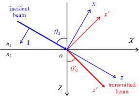
Figure 1: (Color online) Reference frames $xyz$, $x^{\prime}y^{\prime}z^{\prime}$, and $XYZ$ associated, respectively, with the incident beam, the refracted beam, and the laboratory for the refraction at an interface between two different dielectric media, $n_{1}$ and $n_{2}$.

1. Description of the incident beam. In frame $xyz$, the wave vector of the angular spectrum in the linear approximation is given by $\mathbf{k}=(\begin{array}[]{ccc}k_{x}&k_{y}&k\end{array})^{T}$, where the wave number in medium $n_{1}$ is $k=n_{1}k_{0}$, $k_{0}=2\pi/\lambda_{0}$, and $\lambda_{0}$ is the vacuum wavelength. With $\Theta=-\frac{\pi}{2}$, the linearly approximated mapping matrix (7) becomes

$$m=-\left(\begin{array}[]{cc}1&0\\ 0&1\\ -\frac{k_{x}}{k}&-\frac{k_{y}}{k}\end{array}\right).$$ (9)

In frame $XYZ$, the wave vector is transformed into

$$\mathbf{k}_{XYZ}=D_{y}(-\theta_{0})\mathbf{k}=\left(\begin{array}[]{c}k\sin\theta_{0}+k_{x}\cos\theta_{0}\\ k_{y}\\ k\cos\theta_{0}-k_{x}\sin\theta_{0}\end{array}\right),$$ (10)

where

$$D_{y}(\vartheta)=\left(\begin{array}[]{ccc}\cos\vartheta&0&-\sin\vartheta\\ 0&1&0\\ \sin\vartheta&0&\cos\vartheta\\ \end{array}\right)$$

is the rotation matrix of the reference frame around the $y$ axis by an angle $\vartheta$. The mapping matrix is correspondingly transformed into $m_{XYZ}=D_{y}(-\theta_{0})m$ and is given by

$$m_{XYZ}=-\left(\begin{array}[]{cc}\cos\theta_{0}-\frac{k_{x}}{k}\sin\theta_{0}&-\frac{k_{y}}{k}\sin\theta_{0}\\ 0&1\\ -\sin\theta_{0}-\frac{k_{x}}{k}\cos\theta_{0}&-\frac{k_{y}}{k}\cos\theta_{0}\end{array}\right).$$ (11)

2. Operations of the refraction to the incident angular spectrum. Refraction includes two kinds of operation to the incident angular spectrum. One is to alter the wave vector and the mapping matrix by rotation, and the other is to change the Jones vector. So the electric vector of the refracted angular spectrum in the frame $XYZ$ can be assumed to be

$$\mathbf{f}^{\prime}_{XYZ}=m^{\prime}_{XYZ}\tilde{\alpha}^{\prime}f^{\prime},$$ (12)

where $\tilde{\alpha}^{\prime}$ is also normalized. Let us look at the former operation in frame $XYZ$. For an incident plane wave of wave vector (10), the incidence plane is formed by the wave vector (10) and the $Z$ axis. So the incidence angle $\theta$ of this plane wave is determined by

$$\cos\theta=\frac{\mathbf{k}_{XYZ}\cdot\mathbf{e}_{Z}}{|\mathbf{k}_{XYZ}|}=\cos\theta_{0}-\frac{k_{x}}{k}\sin\theta_{0}.$$

Denoting by $\theta^{\prime}$ the refraction angle, the Snell law gives

$$\sin\theta^{\prime}=\frac{n_{1}}{n_{2}}\sin\theta=\sin\theta^{\prime}_{0}+\frac{n_{1}}{n_{2}}\frac{k_{x}}{k}\cos\theta_{0}.$$

The unit vector $\mathbf{n}$ perpendicular to this incidence plane is given by

$$\mathbf{n}=\frac{\mathbf{e}_{Z}\times\mathbf{k}_{XYZ}}{|\mathbf{e}_{Z}\times\mathbf{k}_{XYZ}|}\approx\mathbf{e}_{y}-\frac{k_{y}}{k\sin\theta_{0}}\mathbf{e}_{x}$$

in the linear approximation. Denoting $\Delta\theta=\theta^{\prime}-\theta$, the direction of the refracted wave vector is obtained through rotating the incident wave vector around $\mathbf{n}$ by an angle $\Delta\theta$ within the frame $XYZ$. The wave number is changed by the refraction into $k^{\prime}=\frac{n_{2}}{n_{1}}k=n_{2}k_{0}$. As a result, the refracted wave vector in the frame $XYZ$ is given by

$$\mathbf{k}^{\prime}_{XYZ}=\frac{n_{2}}{n_{1}}D^{-1}_{\mathbf{n}}(\Delta\theta)\mathbf{k}_{XYZ},$$

where

$$D^{-1}_{\mathbf{n}}(\Delta\theta)=\left(\begin{array}[]{ccc}\cos\Delta\theta&-\frac{k_{y}}{k\sin\theta_{0}}(1-\cos\Delta\theta)&\sin\Delta\theta\\ -\frac{k_{y}}{k\sin\theta_{0}}(1-\cos\Delta\theta)&1&\frac{k_{y}}{k\sin\theta_{0}}\sin\Delta\theta\\ -\sin\Delta\theta&-\frac{k_{y}}{k\sin\theta_{0}}\sin\Delta\theta&\cos\Delta\theta\end{array}\right).$$

Correspondingly, the mapping matrix of the refracted plane wave is obtained through the same rotation and is given by

$$m^{\prime}_{XYZ}=D^{-1}_{\mathbf{n}}(\Delta\theta)m_{XYZ}.$$

Now we look at the latter operation. Eq. (11) shows that the first and the second column vectors of the mapping matrix are $p$- and $s$-polarized, respectively, in the zeroth-order approximation. So the refraction converts the normalized Jones vector of the incident beam into $T\tilde{\alpha}$, where $T=\left(\begin{array}[]{cc}t_{p}&0\\ 0&t_{s}\end{array}\right)$,

$$t_{p}=\frac{2\sin\theta^{\prime}_{0}\cos\theta_{0}}{\sin(\theta_{0}+\theta^{\prime}_{0})\cos(\theta_{0}-\theta^{\prime}_{0})}$$

is the Fresnel transmission coefficient of the $p$-polarization, and

$$t_{s}=\frac{2\sin\theta^{\prime}_{0}\cos\theta_{0}}{\sin(\theta_{0}+\theta^{\prime}_{0})}$$

is the Fresnel transmission coefficient of the $s$-polarization. Introducing the normalized Jones vector,

$$\tilde{\alpha}^{\prime}=\frac{1}{N}T\tilde{\alpha}\equiv\left(\begin{array}[]{c}\alpha^{\prime}_{p}\\ \alpha^{\prime}_{s}\end{array}\right),$$ (13)

where $N=(|t_{p}\alpha_{p}|^{2}+|t_{s}\alpha_{s}|^{2})^{1/2}$ is the normalization coefficient, the amplitude scalar $f^{\prime}$ in the electric vector (12) is given by

$$f^{\prime}=Nf.$$ (14)

Eq. (13) means that the polarization ellipticity of the refracted angular spectrum is different from that of the incident angular spectrum and turns out to be

$$\sigma^{\prime}=\tilde{\alpha}^{\prime{\dagger}}\hat{\sigma}\tilde{\alpha}^{\prime}=\frac{t_{p}t_{s}}{N^{2}}\sigma,$$ (15)

noticing that $t_{p}$ and $t_{s}$ are both real numbers.

3. Description of the refracted beam in frame $x^{\prime}y^{\prime}z^{\prime}$. The wave vector of the refracted angular spectrum is transformed into

$$\mathbf{k}^{\prime}\equiv\left(\begin{array}[]{c}k^{\prime}_{x^{\prime}}\\ k^{\prime}_{y^{\prime}}\\ k^{\prime}_{z^{\prime}}\end{array}\right)=D_{y}(\theta^{\prime}_{0})\mathbf{k}^{\prime}_{XYZ}=\left(\begin{array}[]{c}\frac{\cos\theta_{0}}{\cos\theta^{\prime}_{0}}k_{x}\\ k_{y}\\ k^{\prime}\end{array}\right).$$ (16)

The mapping matrix is transformed in the same way, $m^{\prime}=D_{y}(\theta^{\prime}_{0})m^{\prime}_{XYZ}$, and is expressed in terms of $\mathbf{k}^{\prime}$ as follows,

$$m^{\prime}=-\left(\begin{array}[]{cc}1&\frac{k^{\prime}_{y^{\prime}}}{k^{\prime}}\frac{\cos\theta_{0}-\cos\theta^{\prime}_{0}}{\sin\theta^{\prime}_{0}}\\ -\frac{k^{\prime}_{y^{\prime}}}{k^{\prime}}\frac{\cos\theta_{0}-\cos\theta^{\prime}_{0}}{\sin\theta^{\prime}_{0}}&1\\ -\frac{k^{\prime}_{x^{\prime}}}{k^{\prime}}&-\frac{k^{\prime}_{y^{\prime}}}{k^{\prime}}\end{array}\right).$$ (17)

Finally, we arrive at the electric vector of the refracted angular spectrum in the frame $x^{\prime}y^{\prime}z^{\prime}$,

$$\mathbf{f}^{\prime}=m^{\prime}\tilde{\alpha}^{\prime}f^{\prime},$$ (18)

where $m^{\prime}$, $\tilde{\alpha}^{\prime}$, and $f^{\prime}$ are given by Eqs. (17), (13), and (14), respectively. Comparison of Eq. (17) with Eq. (7) shows that the symmetry axis $\mathbf{I}^{\prime}$ of the refracted beam lies in the plane $z^{\prime}ox^{\prime}$, that is to say, in the incidence plane. The angle $\Theta^{\prime}$ between $\mathbf{I}^{\prime}$ and the propagation axis is determined by

$$\cot\Theta^{\prime}=\frac{\cos\theta_{0}-\cos\theta^{\prime}_{0}}{\sin\theta^{\prime}_{0}},$$ (19)

and is no longer equal to $-\frac{\pi}{2}$.

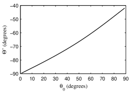
Figure 2: Dependence of $\Theta^{\prime}$ on the incidence angle $\theta_{0}$ for $n_{1}=1$ and $n_{2}=1.515$.

The dependence of $\Theta^{\prime}$ on the incidence angle $\theta_{0}$ is shown in Fig. 2 for $n_{1}=1$ and $n_{2}=1.515$.

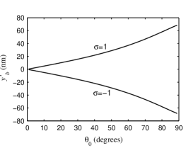
Figure 3: Dependence of $y^{\prime}_{b}$ on the incidence angle $\theta_{0}$ for experimental parameters: $n_{1}=1$, $n_{2}=1.515$, and $\lambda_{0}=633$nm.

According to Eq. (8), the displacement of the refracted beam’s barycenter from the incidence plane is

$$y^{\prime}_{b}=-\frac{\sigma^{\prime}}{k^{\prime}}\cot\Theta^{\prime}.$$ (20)

This is nothing but the Imbert-Fedorov displacement. With $n_{1}=1$, $n_{2}=1.515$, and $\lambda_{0}=633$nm, the dependence of $y^{\prime}_{b}$ on the incidence angle $\theta_{0}$ for $\sigma=\pm 1$ is shown in Fig. 3, which is in quantitative agreement with the experimental data Hosten-K .

Indistinguishableness of different perpendicular $\mathbf{I}$—When Hosten and Kwiat performed their experiment, they did not realize the existence of $\mathbf{I}$. So it was not ensured that the $\mathbf{I}$ of their incident beam lay in the incidence plane. In the following, I will show that incident beams of different perpendicular $\mathbf{I}$ are indistinguishable in the Imbert-Fedorov effect.

For an arbitrary perpendicular symmetry axis, $\mathbf{I}=-\mathbf{e}_{x}\cos\Phi-\mathbf{e}_{y}\sin\Phi$, the mapping matrix in the linear approximation is given by

$$m=\left(\begin{array}[]{cc}-\cos\Phi&\sin\Phi\\ -\sin\Phi&-\cos\Phi\\ \frac{k_{x}}{k}\cos\Phi+\frac{k_{y}}{k}\sin\Phi&\frac{k_{y}}{k}\cos\Phi-\frac{k_{x}}{k}\sin\Phi\end{array}\right).$$ (21)

Inserting a unit $2\times 2$ matrix $I=Q^{T}Q$ into the right-hand side of Eq. (2), one has

$$\mathbf{f}=mQ^{T}Q\tilde{\alpha}f\equiv m^{\prime\prime}\tilde{\alpha}^{\prime\prime}f,$$ (22)

where

$$Q=\left(\begin{array}[]{cc}\cos\Phi&-\sin\Phi\\ \sin\Phi&\cos\Phi\end{array}\right)$$ (23)

is a rotation matrix in the Jones-vector space, $m^{\prime\prime}=mQ^{T}$, and $\tilde{\alpha}^{\prime\prime}=Q\tilde{\alpha}\equiv\left(\begin{array}[]{c}\alpha^{\prime\prime}_{p}\\ \alpha^{\prime\prime}_{s}\end{array}\right)$. Eq. (22) means that the electric vector of the angular spectrum can be expressed either in terms of $m$ together with Jones vector $\tilde{\alpha}$ or in terms of $m^{\prime\prime}$ together with Jones vector $\tilde{\alpha}^{\prime\prime}$. With Eqs. (21) and (23), one has

$$m^{\prime\prime}=-\left(\begin{array}[]{cc}1&0\\ 0&1\\ -\frac{k_{x}}{k}&-\frac{k_{y}}{k}\end{array}\right),$$ (24)

which is the same as the mapping matrix (9). At the same time, rotation $Q$ does not change the polarization ellipticity,

$$\sigma^{\prime\prime}=\tilde{\alpha}^{\prime\prime{\dagger}}\hat{\sigma}\tilde{\alpha}^{\prime\prime}=\tilde{\alpha}^{{\dagger}}Q^{T}\hat{\sigma}Q\tilde{\alpha}=\tilde{\alpha}^{{\dagger}}\hat{\sigma}\tilde{\alpha}=\sigma.$$ (25)

It is thus clear that when the perpendicular $\mathbf{I}$ of the incident beam is rotated around its propagation axis, the linearly approximated mapping matrix and the polarization ellipticity can be regarded as remaining unchanged, resulting in the same Imbert-Fedorov displacement (20).

This work was supported in part by the National Natural Science Foundation of China (60877055 and 60806041), the Science and Technology Commission of Shanghai Municipal (08JC14097 and 08QA14030), the Shanghai Educational Development Foundation (2007CG52), and the Shanghai Leading Academic Discipline Project (S30105).

References

(1) A. Ashkin, IEEE J. Sel. Top. Quantum Electron. 6, 841 (2000).
(2) L. Paterson et al., Science 292, 912 (2001).
(3) X. Xu, K. Kim, W. Jhe, and N. Kwon, Phys. Rev. A 63, 063401 (2001).
(4) D. P. Biss, K. S. Youngworth, and T. G. Brown, Appl. Opt. 45, 470 (2006).
(5) M. Lax, W. H. Louisell, and W. B. McKnight, Phys. Rev. A 11, 1365 (1975).
(6) L. W. Davis, Phys. Rev. A 19, 1177 (1979).
(7) D. N. Pattanayak and G. P. Agrawal, Phys. Rev. A 22, 1159 (1980).
(8) L. W. Davis and G. Patsakos, Opt. Lett. 6, 22 (1981).
(9) R. H. Jordan and D. G. Hall, Opt. Lett. 19, 427 (1994).
(10) K. S. Youngworth and T. G. Brown, Opt. Express 7, 77 (2000).
(11) M. Onoda, S. Murakami, and N. Nagaosa, Phys. Rev. E 74, 066610 (2006).
(12) K. Yu. Bliokh and Yu. P. Bliokh, Phys. Rev. E 75, 066609 (2007).
(13) C.-F. Li, Opt. Lett. 32, 3543 (2007).
(14) H. S. Green and E. Wolf, Proc. Phys. Soc. London Sec. A 66, 1129 (1953).
(15) H. Kogelnik, Appl. Opt. 4, 1562 (1965).
(16) H. Kogelnik and T. Li, Appl. Opt. 5, 1550 (1966).
(17) R. C. Jones, J. Opt. Soc. Am. 31, 488 (1941).
(18) C.-F. Li, Phys. Rev. A 78, 063831 (2008).
(19) H. Ren, Y.-H. Lin, and S.-T. Wu, Appl. Phys. Lett. 89, 051114 (2006).
(20) O. Hosten and P. Kwiat, Science 319, 787 (2008).
(21) F. I. Fedorov, Dokl. Akad. Nauk SSSR 105, 465 (1955).